Course 4 May 2000 Multiple Choice Exams

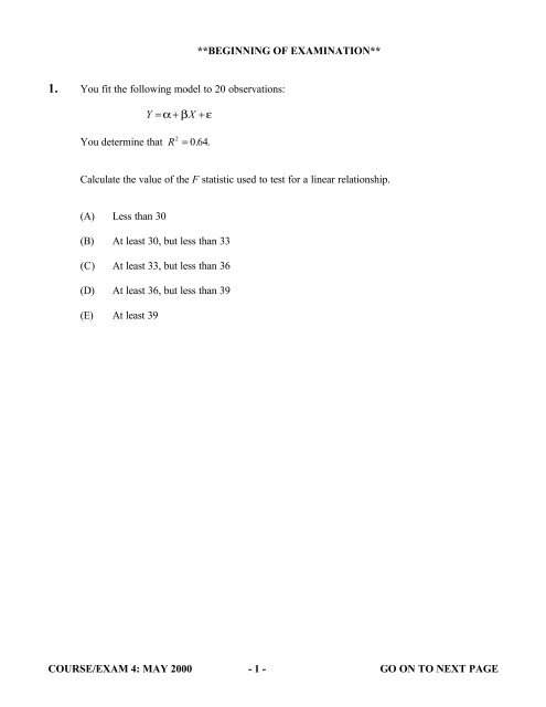
**BEGINNING OF EXAMINATION** 

1. You fit the following model to 20 observations: 

Y = α+ βX 

+ ε 

You determine that R 2 = 0. 64. 

Calculate the value of the F statistic used to test for a linear relationship. 

(A) Less than 30 

(B) At least 30, but less than 33 

(C) At least 33, but less than 36 

(D) At least 36, but less than 39 

(E) At least 39 

COURSE/EXAM 4: MAY 2000 - 1 - GO ON TO NEXT PAGE

2. You are given the following random sample of ten claims: 

46 121 493 738 775 

1078 1452 2054 2199 3207 

Determine the smoothed empirical estimate of the 90 th percentile, as defined in Klugman, Panjer 

and Willmot. 







3. You are given the following information about two classes of business, where X is the loss for an 

individual insured: 

Class 1 Class 2 

Number of insureds 25 50 

b g 380 23 

c h 365,000 ---- 

E X 

E X 2 

You are also given that an analysis has resulted in a Bühlmann k value of 2.65. 

Calculate the process variance for Class 2. 

(A) 2,280 

(B) 2,810 

(C) 7,280 

(D) 28,320 

(E) 75,050 


4. For a mortality study with right-censored data, you are given: 

Time 

t i 

5 

7 

10 

12 

Number of Deaths 

d i 

2 

1 

1 

2 

Number at Risk 

Y i 

15 

12 

10 

6 

Calculate ~ S 12 

b g based on the Nelson-Aalen estimate H ~ b12g. 

(A) 0.48 

(B) 0.52 

(C) 0.60 

(D) 0.65 

(E) 0.67 


5. You are given the following information about an MA(4) model: 

m 

q1 

q2 

q3 

q4 

2 

s e 

= 

= 

= 

= 

= 

= 

0 

1800 . 

−1110 

. 

0. 

278 

−0. 

024 

8. 

000 

Determine the standard deviation of the forecast error three steps ahead. 

(A) 2.8 

(B) 3.6 

(C) 4.9 

(D) 5.8 

(E) 6.6 


6. A jewelry store has obtained two separate insurance policies that together provide full coverage. 

You are given: 

(i) The average ground-up loss is 11,100. 

(ii) 

Policy A has an ordinary deductible of 5,000 with no policy limit. 

(iii) Under policy A, the expected amount paid per loss is 6,500. 

(iv) Under policy A, the expected amount paid per payment is 10,000. 

(v) Policy B has no deductible and a policy limit of 5,000. 

Given that a loss less than or equal to 5,000 has occurred, what is the expected payment under 

policy B? 

(A) Less than 2,500 

(B) At least 2,500, but less than 3,000 

(C) At least 3,000, but less than 3,500 

(D) At least 3,500, but less than 4,000 

(E) At least 4,000 


7. You are given the following information about two classes of risks: 

(i) 

(ii) 

Risks in Class A have a Poisson claim count distribution with a mean of 1.0 per year. 

Risks in Class B have a Poisson claim count distribution with a mean of 3.0 per year. 

(iii) Risks in Class A have an exponential severity distribution with a mean of 1.0. 

(iv) Risks in Class B have an exponential severity distribution with a mean of 3.0. 

(v) 

(vi) 

Each class has the same number of risks. 

Within each class, severities and claim counts are independent. 

A risk is randomly selected and observed to have two claims during one year. The observed 

claim amounts were 1.0 and 3.0. 

Calculate the posterior expected value of the aggregate loss for this risk during the next year. 

(A) Less than 2.0 

(B) At least 2.0, but less than 4.0 

(C) At least 4.0, but less than 6.0 

(D) At least 6.0, but less than 8.0 

(E) At least 8.0 


8. You are given the following data on time to death: 

(i) 

Time 

t i 


d i 

Number of Risks 

Y i 

( t i 

) 

H ~ 

10 1 20 0.0500 

34 1 19 0.1026 

47 1 18 0.1582 

75 1 17 0.2170 

156 1 16 0.2795 

171 1 15 0.3462 

(ii) H ~ ( t i 

) 

is the Nelson-Aalen estimate of the cumulative hazard function. 

(iii) h $ ( t ), the kernel-smoothed estimate of the hazard rate, is determined using bandwidth 60 

and the uniform kernel 

K 

( x ) 

= 

R 

S| 

T| 

1 

2 

, 

− 1 ≤ x ≤ 1 

0 , o t h e r w i s e . 

Determine h $ ( 100 ) . 

(A) 0.0010 

(B) 0.0015 

(C) 0.0029 

(D) 0.0590 

(E) 0.0885 


9. The following models are fitted to 30 observations: 


Model I: Y = β + β X + ε 

1 2 2 

Model II: Y = β + β X + β X + β X + ε 

(i) ∑cY − Yh = 160 

(ii) 

2 

∑c X2 X2h 

− = 10 

(iii) For Model I, β $ 2 

= −2 

1 2 2 3 3 4 4 

(iv) For Model II, R 2 = 070 . 

Determine the value of the F statistic used to test that β 3 

and β 4 

are jointly equal to zero. 







10-11. Use the following information for questions 10 and 11. 

The size of a claim for an individual insured follows an inverse exponential distribution with the 

following probability density function: 

θ −θ 

x 

e 

f ( x θ) = , x > 

x 

2 

0 

The parameter θ has a prior distribution with the following probability density function: 

−θ 

e 

gbθg 4 

= , θ > 0 

4 

10. For question 10 only, you are also given: 

One claim of size 2 has been observed for a particular insured. 

Which of the following is proportional to the posterior distribution of θ? 

(A) 

θe −θ 

2 

(B) θ θ 

e −3 4 

(C) 

(D) 

(E) 

θe −θ 

θ 

θ 

2 

θ 

e − 2 

2 

θ 

e −9 4 


10-11. (Repeated for convenience) Use the following information for questions 10 and 11. 

The size of a claim for an individual insured follows an inverse exponential distribution with the 

following probability density function: 

θ −θ 

x 

e 

f ( x θ) = , x > 

x 

2 

0 

The parameter θ has a prior distribution with the following probability density function: 

−θ 

e 

gbθg 4 

= , θ > 0 

4 

11. For question 11 only, you are also given: 

For a particular insured, the following five claims are observed: 

1 2 3 5 13 

Determine the value of the Kolmogorov-Smirnov statistic to test the goodness of fit of 

f xθ = 2 c h. 







12. For a mortality study, you are given: 

(i) 

(ii) 

(iii) 

(iv) 

(v) 

100 newborn mice are observed for four months. 

H 0 is a hypothesized cumulative hazard function. 

Deaths during the month are assumed to occur at the end of the month. 

The 95 th percentile of the chi-square distribution with one degree of freedom 

is 3.84. 

The observed mortality experience and the values of H 0 are given below. 

Month 

Number at 

beginning of month 

Number 

of deaths 

H 0, beginning 

of month 

H 0, end 

of month 

1 100 10 0.00 0.08 

2 90 12 0.08 0.15 

3 78 10 0.15 0.25 

4 68 d 4 0.25 0.40 

Calculate the smallest value of d 4 needed for the one-sample log-rank test to yield the 

conclusion, at the 0.05 significance level, that the true cumulative hazard function differs 

from H 0 . 

(A) 0 

(B) 3 

(C) 6 

(D) 9 

(E) 12 


13. You smooth a time series y t 

using Holt’s two-parameter exponential smoothing method. 

You calculate: 

t 

yt 

y~ 

t 

r t 

1995 120.5 120.0 10.0 

1996 135.0 131.5 11.2 

1997 147.7 144.2 12.4 

1998 146.6 

~ y1998 r 1998 

Determine the two-period forecast $y 2000 by first completing Holt’s two-parameter exponential 

smoothed series. 







14. Which of the following statements about evaluating an estimator is false? 

(A) 

Modeling error is not possible with empirical estimation. 

^ ^ ^) 

(B) MSE( θ) = Var( θ) + Bias( 

θ 

n 

2 1 

2 

(C) Sn 

= ∑d X 

j 

− Xi is an asymptotically unbiased estimator of variance. 

n 

(D) 

j= 

1 

If θ^n is asymptotically unbiased and limVar( θ ) = 

2 

n →∞ 

^ 

n 

^ 

0, then θ n 

is weakly consistent. 

(E) 

A robust estimator is one that performs well even with sampling error. 


15. An insurer has data on losses for four policyholders for seven years. X ij is the loss from 

the i th policyholder for year j. 


4 

∑∑ 

i= 

1 

7 

j= 

1 

d 

X 

ij 

− X = 33. 

60 

i 

i 

2 

4 

∑ 

i= 

1 

c 

X 

i 

h 

2 

− X = 3. 

30 

Calculate the Bühlmann credibility factor for an individual policyholder using nonparametric 

empirical Bayes estimation. 







16. You are given: 

(i) 

x 1 = −2 

x 2 = −1 

x 3 = 0 

x 4 = 1 

x 5 = 2 

(ii) The true model for the data is y = 10x + 3x 

2 + ε . 

* * . 

(iii) The model fitted to the data is y = β x + ε 

Determine the expected value of the least-squares estimator of β * . 

(A) 6 

(B) 7 

(C) 8 

(D) 9 

(E) 10 


17. You are given a random sample of two values from a distribution function F: 

1 3 

b g 

You estimate θ F 

X 

X = 

+ X 

2 

1 2 

. 

2 

1 

= Var b Xg 

using the estimator g( X1, X2) = ∑ ( Xi 

− X ) 

2 

i= 

1 

2 

, where 

Determine the bootstrap approximation to the mean square error. 

(A) 0.0 

(B) 0.5 

(C) 1.0 

(D) 2.0 

(E) 2.5 


18. You are given two independent estimates of an unknown quantityµ: 

b g 

b g 

b g 

b g 

(i) Estimate A: E µ A 

= 1000 and σ µ A 

= 400 

(ii) Estimate B: E µ B 

= 1200 and σ µ B 

= 200 

Estimate C is a weighted average of the two estimates A and B, such that: 

µ = w⋅ µ + 1− w ⋅µ 

C A B 

b 

g 

Determine the value of w that minimizes σ bµ C g . 

(A) 0 

(B) 1/5 

(C) 1/4 

(D) 1/3 

(E) 1/2 


19. For a mortality study with right-censored data, the cumulative hazard rate is estimated using the 

Nelson-Aalen estimator. 


(i) No deaths occur between times t i and t i+1 . 

(ii) A 95% linear confidence interval for H(t i ) is (0.07125, 0.22875). 

(iii) A 95% linear confidence interval for H(t i+1 ) is (0.15607, 0.38635). 

Calculate the number of deaths observed at time t i+1 . 

(A) 4 

(B) 5 

(C) 6 

(D) 7 

(E) 8 


20. For the time series y t , you are given: 

t y t 

yt − y 

1 984 −16 

2 1023 23 

3 965 −35 

4 1040 40 

5 988 −12 

Estimate the partial autocorrelation function at time displacement k = 2 . 

(A) −0.46 

(B) −0.16 

(C) 0.00 

(D) 0.51 

(E) 0.84 


21. You are given the following five observations: 

521 658 702 819 1217 

You use the single-parameter Pareto with cumulative distribution function 

Fbxg F = − x 

H G α 

500 

1 

I 

x K J , > 500, α > 0. 

Calculate the maximum likelihood estimate of the parameter α . 

(A) 2.2 

(B) 2.5 

(C) 2.8 

(D) 3.1 

(E) 3.4 



(i) A portfolio of independent risks is divided into two classes, Class A and Class B. 

(ii) There are twice as many risks in Class A as in Class B. 

(iii) 

(iv) 

The number of claims for each insured during a single year follows a Bernoulli 

distribution. 

Classes A and B have claim size distributions as follows: 

Claim Size Class A Class B 

50,000 0.60 0.36 

100,000 0.40 0.64 

(v) The expected number of claims per year is 0.22 for Class A and 0.11 for Class B. 

One insured is chosen at random. The insured’s loss for two years combined is 100,000. 

Calculate the probability that the selected insured belongs to Class A. 

(A) 0.55 

(B) 0.57 

(C) 0.67 

(D) 0.71 

(E) 0.73 


23. You test the effect of gender and age on survival of patients receiving kidney transplants. 

(i) 

(ii) 

You use a Cox proportional hazards model with the indicator variable Z 1 

equal to 1 when 

the subject is a male, and the indicator variable Z 2 

equal to 1 when the subject is an adult. 

The resulting partial maximum likelihood parameter estimates are: 

b 1 = 0.25 

b 2 = −0.45 

(iii) 

The variance-covariance matrix of b 1 and b 2 is given by: 

F 

HG 

036 . 010 . 

010 . 020 . 

I 

KJ 

Which of the following is a 95% confidence interval for the relative risk of a male child subject 

compared to a female adult subject? 

(A) (−0.5, 1.9) 

(B) (0.0, 1.4) 

(C) (0.6, 6.5) 

(D) (1.0, 4.1) 

(E) (1.2, 3.2) 


24. You are given the following linear regression results: 

t Actual Fitted 

1 77.0 77.6 

2 69.9 70.6 

3 73.2 70.9 

4 72.7 72.7 

5 66.1 67.1 

Estimate the lag 1 serial correlation coefficient for the residuals, using the Durbin-Watson 

statistic. 

(A) Less than −0.2 

(B) At least −0.2, but less than −0.1 

(C) At least −0.1, but less than 0.0 




25. You model a loss process using a lognormal distribution with parameters µ and σ . 


(i) 

The maximum likelihood estimates of µ and σ are: 

^ 

µ 

^ 

σ 

= 4. 

215 

= 1093 . 

(ii) The estimated covariance matrix of µ^ and σ^ is: 

⎛01195 . 0 ⎞ 

⎜ 

⎟ 

⎝ 0 0. 

0597⎠ 

(iii) The mean of the lognormal distribution is exp( µ + σ 2 

) 

2 . 

Estimate the variance of the maximum likelihood estimate of the mean of the lognormal 

distribution, using the delta method. 


(B) At least 1500, but less than 2000 

(C) At least 2000, but less than 2500 





(i) 

Claim counts follow a Poisson distribution. 

(ii) Claim sizes follow a lognormal distribution with coefficient of variation 3. 

(iii) 

Claim sizes and claim counts are independent. 

(iv) The number of claims in the first year was 1000. 

(v) 

(vi) 

(vii) 

(viii) 

The aggregate loss in the first year was 6.75 million. 

The manual premium for the first year was 5.00 million. 

The exposure in the second year is identical to the exposure in the first year. 

The full credibility standard is to be within 5% of the expected aggregate loss 95% of the 

time. 

Determine the limited fluctuation credibility net premium (in millions) for the second year. 







27. You are analyzing the time between the occurrence and payment of claims. You are given the 

following data on four claims that were paid during the time period t = 0 to 

t = 6 (in months): 

Time of occurrence 

(t) 

Time between 

occurrence and 

payment 

3 1 

5 1 

3 2 

2 3 

You have no information on claims that occurred during the period t = 0 to t = 6 but were not 

paid until after t = 6. 

Given that a claim is paid no later than six months after its occurrence, using the appropriate 

form of the Product-Limit estimator, estimate the probability that the claim is paid less than two 

months after its occurrence. 

(A) 0 

(B) 1/4 

(C) 1/3 

(D) 1/2 

(E) 2/3 


28. You are given two time series, xt 

and y t 

. Each time series is assumed to be a random walk. 

Which of the following statements about these series is correct? 

(A) 

No linear combination of these two time series can be stationary. 

(B) The time series zt = xt − λ yt 

is always stationary for some value λ. 

(C) The time series zt = xt − λ yt 

may be stationary for some value λ that can be determined 

precisely using regression techniques. 

(D) The time series zt = xt − λ yt 

may be stationary for some value λ that can be estimated 

by running an ordinary least-squares regression of x 

t 

on y 

t 

. 

(E) 

None of (A), (B), (C) or (D) is correct. 


29. You are given the following observed claim frequency data collected over a period of 365 days: 

Number of Claims per Day 

Observed Number of Days 

0 50 

1 122 

2 101 

3 92 

4+ 0 

Fit a Poisson distribution to the above data, using the method of maximum likelihood. 

Group the data by number of claims per day into four groups: 

0 1 2 3 or more 

Apply the chi-square goodness-of-fit test to evaluate the null hypothesis that the claims follow a 

Poisson distribution. 

Determine the result of the chi-square test. 

(A) 

(B) 

(C) 

(D) 

(E) 

Reject at the 0.005 significance level. 

Reject at the 0.010 significance level, but not at the 0.005 level. 



Do not reject at the 0.050 significance level. 



(i) 

An individual automobile insured has an annual claim frequency distribution that follows 

a Poisson distribution with mean λ. 

(ii) λ follows a gamma distribution with parametersαand θ. 

(iii) The first actuary assumes that α =1 and θ = 1/6. 

(iv) 

(v) 

(vi) 

The second actuary assumes the same mean for the gamma distribution, but only half the 

variance. 

A total of one claim is observed for the insured over a three year period. 

Both actuaries determine the Bayesian premium for the expected number of claims in the 

next year using their model assumptions. 

Determine the ratio of the Bayesian premium that the first actuary calculates to the Bayesian 

premium that the second actuary calculates. 

(A) 3/4 

(B) 9/11 

(C) 10/9 

(D) 11/9 

(E) 4/3 




Y = β + β X + β X + β X + ε 

1 2 2 3 3 4 4 

Source 

of Variation 

Degrees 

of Freedom 

Sum 

of Squares 

Regression 3 103,658 

Error 44 69,204 

Calculate R 2 , the corrected R 2 . 

(A) 0.57 

(B) 0.58 

(C) 0.59 

(D) 0.60 

(E) 0.61 


32. You are given the following information about a sample of data: 

(i) Mean = 35,000 

(ii) Standard deviation = 75,000 

(iii) Median = 10,000 

(iv) 90 th percentile = 100,000 

(v) 

The sample is assumed to be from a Weibull distribution. 

Determine the percentile matching estimate of the parameter τ . 







33. The number of claims a driver has during the year is assumed to be Poisson distributed with an 

unknown mean that varies by driver. 

The experience for 100 drivers is as follows: 

Number of Claims 

during the Year 

Number of Drivers 

0 54 

1 33 

2 10 

3 2 

4 1 

Determine the credibility of one year’s experience for a single driver using semiparametric 

empirical Bayes estimation. 

(A) 0.046 

(B) 0.055 

(C) 0.061 

(D) 0.068 

(E) 0.073 


34. In a mortality study, the Weibull distribution with parameters λ and α was used as the survival 

model, and log time Y was modeled as Y = µ + σ W, with W having the standard extreme value 

distribution. The parameters satisfy the relations: 

The maximum likelihood estimates of the parameters are µ^ = 4.13 and σ^ =1.39. 

The estimated variance-covariance matrix of µ 

F 

HG 

^ 

0. 075 0016 . 

0016 . 0048 . 

I 

KJ 

and 

^ 

σ 

is: 

Use the delta method to estimate the covariance of α^ 

and lnd ^λ i. 

(A) Less than −0.054 

(B) At least −0.054, but less than −0.018 

(C) At least −0.018, but less than 0.018 





(i) s 2 = 10 

Y = β + β X + β X + ε 

1 2 2 3 3 

(ii) 

r x 2 x 

= 0. 

5 

3 

∑ 

2 

(iii) ( X − X ) = 4 

∑ 

2 2 

2 

(iv) ( X − X ) = 8 

3 3 

Determine the estimate of the standard deviation of the least-squares estimate of the difference 

between β 2 

and β 3 

. 

(A) 1.7 

(B) 2.2 

(C) 2.7 

(D) 3.2 

(E) 3.7 


36. You are given the following sample of five claims: 

4 5 21 99 421 

You fit a Pareto distribution using the method of moments. 

Determine the 95 th percentile of the fitted distribution. 








(i) 

X i 

is the claim count observed for driver i for one year. 

(ii) X i 

has a negative binomial distribution with parameters β = 0.5 and r i . 

(iii) 

µ i 

is the expected claim count for driver i for one year. 

(iv) The µ i ’s have an exponential distribution with mean 0.2. 

Determine the Bühlmann credibility factor for an individual driver for one year. 







38. A mortality study is conducted on 50 lives observed from time zero. 


(i) 

Time 

t 


d t 

Number Censored 

c t 

15 2 0 

17 0 3 

25 4 0 

30 0 c 30 

32 8 0 

40 2 0 

(ii) S $ b 35 g is the Product-Limit estimate of Sb35g . 

(iii) V$ S$ 

b35g is the estimate of the variance of S $ b35g using Greenwood’s formula. 

(iv) 

b g 

2 

b g 

V$ S$ 

35 

S$ 

35 

= 0. 

011467 

Determine c 30 , the number censored at time 30. 

(A) 3 

(B) 6 

(C) 7 

(D) 8 

(E) 11 


39. You fit an AR(1) model to the following data: 

y 

y 

y 

y 

y 

1 

2 

3 

4 

5 

= 2. 

0 

= −1.7 

= 1.5 

= −2.0 

= 1.5 

You choose as initial valuesε = 0, µ = 0 and ρ = 0.5. 

1 1 

2 

Determine the value of the sum of squares function S = ∑ εt 

ε 

1 

= 0, µ = 0, ρ1 

= 05 . . 

(A) 2 

(B) 12 

(C) 15 

(D) 21 

(E) 27 


40. You are given the following accident data from 1000 insurance policies: 

Number of accidents Number of policies 

0 100 

1 267 

2 311 

3 208 

4 87 

5 23 

6 4 

7+ 0 

Total 1000 

Which of the following distributions would be the most appropriate model for this data? 

(A) 

(B) 

(C) 

(D) 

(E) 

Binomial 

Poisson 

Negative Binomial 

Normal 

Gamma 

**END OF EXAMINATION** 

COURSE/EXAM 4: MAY 2000 - 40 - STOP

Solutions to May 2000 Course 4 Exam 

When referencing textbooks, KM = Survival Analysis, KPW = Loss Models, PR = 

Econometric Models and Economic Forecasts, R = Simulation 

1. From (4.12) on p. 91 of PR, 

.64 20 2 

F = = = 32 . (B) 

2 

R N −k 

− 

2 

1−R 

k −1 1 −.64 2−1 

RSS /( k−1) 

2 

Alternatively, from the three definitions, F = 

, R = RSS / TSS , and 

ESS /( N − k ) 

TSS = RSS + ESS , it is possible to use the given information to solve for F. 

2. From Definition 2.14 on p. 35 of KPW, g = [11(.9)] = 9, h = 11(.9) − 9 = .9 and 

π ˆ = .1 + .9 = .1(2199) + .9(3207) = 3106.2 . (D) 

so .9 

x (9) 

x (10) 

3. From (5.60) on p. 437 of KPW, begin with 

EEX [ ( 

j 

| Θ )] = (1/3)(380) + (2/3)(23) = 142 . Then, 

Var EX Θ = + − = . From the definition of k, 

2 2 2 

[ ( 

j 

| )] (1/3)380 (2/3)23 142 28,322 

EVar X 

2 

[ ( 

j 

| )] 2.65(28,322) 75,053.3 (1/3)(365,000 380 ) (2/3) Var( X2) 

Θ = = = − + and 

so Var( X 

2) = 2,280. (A) 

2 1 1 2 

4. From (4.2.3) on p. 86 of KM, H % (12) = + + + = .65 and then also from 

15 12 10 6 

.65 

p. 86, S % (12) = e − = .52 . (B) 

Note that in (4.2.3) the sum is over all death times less than or equal to the time at which 

the survival function is to be evaluated. 

5. For an MA model the ψ ’s are equal to the negatives of the θ ’s. From (18.42) on 

p. 563 of PR, the variance for the three-step-ahead forecast is 

2 2 2 2 2 

(1 + θ1 + θ2) σ ε 

= (1+ 1.8 + 1.11 )(8) = 43.7768. The standard deviation is the square 

root, 6.6164. 

(E) 

6. Using Theorem 2.5 and Corollary 2.6 on p. 74 of KPW, 

6,500 = E( X) −E( X ∧ 5,000) = 11,100 −E( X ∧ 5,000) and so E( X ∧ 5,000) = 4,600. 

E( X) −E( X ∧5,000) 

Also, 10,000 = 

and so F (5,000) = .35 . 

1 − F (5,000) 

Using the definition of conditional expectation, 

5,000 

∫ xf( xdx ) 

0 

E( X ∧5,000) −5,000[1 −F(5,000)] 

E( X| X < 5,000) = = = 3,857 . (D) 

F(5,000) F(5,000)

7. See Example 5.30 on p. 428 of KPW. The calculations use the fact that the number of 

claims and the claim amounts are independent. The goal is to use Bayes’ Theorem to 

obtain Pr( A| N = 2, X1= 1, X2 

= 3) . To do this, we need 

2 −1 

1 e −1 −3 −5 

Pr( N = 2, X1 = 1, X2 

= 3| A) = e e = .5e 

and 

2! 

2 −3 −1/3 −3/3 

3 e e e 

−13/3 

Pr( N = 2, X1 = 1, X2 

= 3| B) = = .5e 

. The answer is then 

2! 3 3 

−5 

.5(.5 e ) 

Pr( A| N = 2, X = 1 

1, X = 2 

3) = .33924 

−5 −13/3 

.5(.5 e ) + .5(.5 e ) 

= . 

For class A, the expected cost is 1(1) = 1 and for class B it is 3(3) = 9. The answer is 

.33924(1) + .66076(9) = 6.286. (D) 

1 t−t 8. From (6.2.4) on p. 153 of KM, ht ˆ( ) = K 

⎛ i ⎞ 

∆Ht 

() 

b 

⎜ 

b 

⎟ 

⎝ ⎠ 

K( x) = .5, −1 ≤x 

≤ 1. The calculation is in the following table: 

t i (100-t i )/60 K ∆ Ht ( i 

) 

10 1.5 0 .05 

34 1.1 0 .0526 

47 .8833 .5 .0556 

75 .4167 .5 .0588 

156 -.9333 .5 .0625 

171 -1.183 0 .0667 

1 

Then, h ˆ(100) = (.5)(.0556 + .0588 + .0625) = .00147 . 

60 

(B) 

9. Method I: From (i), TSS = 160 (using (3.26) on p. 71 of PR), 

from (iv), RSS II = .7(160) = 112 (using (4.9) on p. 89), 

and from (ii) and (iii), RSS I = ( − 2) 2 (10) = 40 (using p. 73). 

Then we have ESS II = 160 − 112 = 48 and ESS I = 160 − 40 = 120. 

(120− 

48)/2 

From (5.20) on p. 129, F = = 19.5 . (C) 

48/(30−4) 

Method II: Use (5.21) on p. 130 along with p. 73 to get 

(.7 − .25)/2 

then F = = 19.5 . 

(1 − .7)/26 

R = ( − 2) (10)/160 = .25 and 

2 2 

I 

10. From Theorem 2.16 on p. 108 of KPW (also as (5.20) on p. 404), 

−θ 

/2 −θ 

/4 

θe 

e 

−.75θ 

πθ ( |2) ∝ f(2| θπθ ) ( ) = ∝ θe 

. (B) 

4 4

11. From pp. 123-5 of KPW and following Example 2.64, 

Observation Empirical cdf- Empirical cdf+ Model cdf Max difference 

1 0 .2 .135 .135 

2 .2 .4 .368 .168 

3 .4 .6 .513 .113 

5 .6 .8 .670 .130 

13 .8 1 .857 .143 

The model cdf is 

∫ 

x 

θ / t 

θ − − 2 − θ / x 

0 

F( x) 

= e t dt = e 

. The overall maximum is the test statistic, 

.168. (D) 

12. From p. 189 of KM begin with O(τ) = number of observed events = 32 + d 4 . The 

other key quantity is E(τ) which is the sum over all lives of the difference in H from 

when they were first seen until when they were last seen. All the lives were first seen at 

age 0. 10 lives were seen from 0 to 1 and contribute10b. 08 − 0g = . 8. The next 12 lives 

each contribute .15. All 68 lives in the final row were last seen at time 4 (some last seen 

alive, some dead). Thus, E() τ = 10(.08) + 12(.15) + 10(.25) + 68(.40) = 32.3 and so the 

test statistic is 

(32+ d4 

−32.3) 

32.3 

2 

> 3.84. Solving this inequality leads to d 4 > 11.437. (E) 

13. Formulas (15.34) and (15.35) on p. 480 of PR are y% t 

= αyt + (1 − α)( y% t−1+ 

rt−1) 

and 

rt = γ( y% t− y% t−1) + (1 −γ) 

rt− 

1. Using the first two rows (the second two rows could also be 

used), 131.5 = α(135.0) + (1 − α)(120.0+ 10.0),for α = .3 and 

11.2 = γ(131.5− 120) + (1 − γ)(10.0),for γ = .8. 

Then, y % 

1998 

= .3(146.6) + .7(144.2+ 12.4) = 153.6 and 

r 

1998 

= .8(153.6− 144.2) + .2(12.4) = 10 . From (15.36), 

yˆ = % y + 2r 

= 153.6+ 2(10) = 173.6. (E) 

2000 1998 1998 

14. (A) is true because there is no model (p. 40 of KPW); (B) is true by (2.9) of KPW; 

(C) is true by p. 43 of KPW; (D) is true by p. 43 of KPW; (E) is false because robustness 

refers to model error (p. 48 of KPW). 

(E) 

1 

15. From (5.75) on p. 464 of KPW, v ˆ = 33.60= 1.4 and from (5.76) on p. 465, 

4(6) 

1 1 

7 

a ˆ = 3.30− 33.6 = .9 . Then, Z = = .818 . (D) 

3 4(7)(6) 

7+ 

1.4/.9 

16. Method I: Use (7.10) from p. 185 of PR. 

E β $ * = β 2 + β 3 x2x3 / x2 2 = 10 + 3 0 / 10 = 10 . 

(E) 

e j 

∑ 

∑ 

b g

∑ 

∑ 

Method II: From basic principles, $ xi 

− x yi 

β * = 

= ∑ xi 

yi. 

x − x 10 

E( y ) = 10x + 3x 

and so 

2 

i i i 

b 

g 

1 

b i g 2 

ˆ 1 

2 

E( β *) = ∑ xi(10xi + 3 xi 

) = 10 . 

10 

Under the true model, 

17. The bootstrap is discussed in both KPW and R. In Section 7.3 of R it is used to 

estimate the mean square error. Following the discussion in R, there are four equally 

likely bootstrap samples, (1,1), (1,3), (3,1), and (3,3). Inserting each sample into the 

estimator yields the four bootstrap estimates, 0, 1, 1, and 0. The estimate using the actual 

sample of (1,3) is 1 and so the estimate of the mean square error is 

1 [(0 1) 

2 (1 1) 

2 (1 1) 

2 (0 1)] 

2 

− + − + − + − = .5 . (B) 

4 

18. Because the estimators are independent, 

2 2 

Var( µ ) = wVar( µ ) + (1 −w) Var( µ ) 

C A B 

= 160,000w 

+ 40,000(1 −w) 

2 2 

2 

= 200,000w 

− 80,000w+ 

40,000. 

The derivative with respect to w is 400,000w− 80,000 and setting it equal to zero gives 

w = .2. A similar example can be found in Exercise 2.21 on p. 160 of KPW. (B) 

19. The intervals are .15 ± .07875 and .27121 ± .11514 . The standard deviations are the 

plus/minus terms divided by 1.96, or .04018 and .05874. From (4.2.4) on p. 86 of KM, 

i 

i+ 

1 

2 2 2 2 

= d 

j 

Yj = d 

j 

Yj 

j= 1 j= 

1 

∑ ∑ and therefore 

.04018 / and .05874 / 

.001836 = d / Y . Also, 

2 

i+ 1 i+ 

1 

from (4.2.3) on p. 86, .27121 − .15 = .12121 = di+ 1/ 

Yi+ 

1. Solving the two equations yields 

2 

d 

i + 1 

= .12121 /.001836= 8. (E) 

20. From Section 17.2.2 on pp. 532-3 of PR, the partial autocorrelation function at k = 2 

is the estimate of φ 2 from an AR(2) model using the Yule-Walker equations. The 

equations require the sample autocorrelations, which can be calculated using (16.23) on 

p. 495. They are: 

− 16(23) + 23( −35) − 35(40) + 40( −12) −3053 

ρˆ 1 

= = =−.813266 

2 2 2 2 2 

16 + 23 + 35 + 40 + 12 3754 

−16( − 35) + 23(40) −35( −12) 1900 

ρˆ 2 

= = = .506127. 

3754 3754 

The Yule-Walker equations are: 

ρ = φ + φρ , − .813266 = φ −.813266φ 

1 1 2 1 1 2 

ρ2 = φρ 

1 1+ φ2, .506127 =− .813266φ1 + φ2 

and solving the equations yields φ 2 = − .46. 

(A)

1 

21. Following Example 2.22 on p. 57 of KPW, f ( x) 500 

α −α− 

= α x and so 

5 5α 

1 

L α 500 ( x ) 

−α 

− 

= ∏ i 

, l = 5lnα+ 5αln500 − ( α+ 1) ∑ln 

xi 

, 

l = 5lnα+ 31.0730α− 33.1111( α+ 1) . Taking the derivative and setting it equal to zero 

yields 

1 

5α 

2.0381 0, αˆ 

2.453 

− − = = . (B) 

22. The solution is taken from formulas in Sections 2.8 and 5.2.5 of KPW as illustrated 

on pp. 425-6. 

Pr(100,000| A) = .22(.4)(.78) + .78(.22)(.4) + .22(.6)(.22)(.6) = .154704 

Pr(100,000| B) = .11(.64)(.89) + .89(.11)(.64) + .11(.36)(.11)(.36) = .126880. 

From Bayes’ Theorem, 

(2/3)(.154704) 

Pr( A |100,000) = = .709. 

(2/3)(.154704) + (1/3)(.126880) 

23. Following p. 248 of KM, a confidence interval for β1− β2 

is given by 

⎛.36 .10⎞⎛ 1 ⎞ 

.25 −( − .45) ± 1.96 ( 1 −1 ) ⎜ .10 .20 ⎟⎜ 

− 1 ⎟ 

⎝ ⎠⎝ ⎠ 

= .7± 1.96 .36 = .7± 

1.176. 

1 2 

The quantity of interest is e β −β 

and so a confidence interval is obtained by 

exponentiating the endpoints of the interval just obtained. That is, 

exp(.7− 1.176) = .62 to exp(.7+ 1.176) = 6.53. (C) 

24. From (6.22) on p. 165 of PR, 

DW = 

∑ 

2 

t − t 

= − + 2 + + 2 + − 2 + − − 

2 

bε$ ε$ 

−1g b . 7 . 6g b23 . . 7g b0 23 . g b 1 0g 

ε$ 

2 

2 2 2 2 2 

t 

− . 6 + − . 7 + 23 . + 0 + −1 

∑ 

b g b g 

b g 

153 . 

= = 2143 . . 

714 . 

From text material on p. 165, DW is approximately 2(1 − ρˆ 

) and so 

ρ ˆ = 1− 2.143/2 =− .0715. (C) 

25. Use Theorem 2.3 on p. 67 of KPW as illustrated in Example 2.26 on that page. The 

reference to the “delta method” is in the second paragraph. 

g( µσ , ) = e 

2 

µ + σ /2 

2 

µ + σ /2 

∂g/ ∂ µ = e = 123.017 

2 

µ + σ /2 

∂g/ ∂ σ = σe 

= 134.458. 

Then the variance is 

⎛.1195 0 ⎞⎛123.017⎞ ( 123.017 134.458) ⎜ = 2887.73 

0 .0597 

⎟⎜ 

134.458 

⎟ . (D) 

⎝ ⎠⎝ ⎠ 

(D)

26. From pp. 412-3 of KPW, the credibility standard for expected claims is 

⎛1.96 

⎞ 

⎜ 

.05 

⎟ 

⎝ ⎠ 

2 

2 

(1+ 3) = 15,366.4. 

Using the square root rule from pp. 416-7, 

Z = 1000/15366.4 = .255. The credibility premium is .255(6.75) + .745(5) = 5.45. (A) 

27. This data is right-truncated, so following the format of Table 5.5 on p. 136 of KM: 

T i X i R i d i Y i Pr $ X < xi 

X ≤ 6 

3 1 5 

5 1 5 2 2 0 

3 2 4 1 2 1/3 

2 3 3 1 3 2/3 

The key to the problem is to observe that the second observation cannot be included in 

the last two entries of the Y i column because the time of the occurrence is too late in the 

observation period. From the last column of the table, the answer is 1/3. 

(C) 

28. See pp. 513-4 of PR. 

(A) is incorrect because some time series are co-integrated. 

(B) is incorrect because a co-integrating parameter will not exist in all cases. 

(C) is incorrect because, even if two series are co-integrated, the co-integrating 

parameter cannot be determined precisely. 

(D) is correct. 

(E) is incorrect because (D) is correct. (D) 

29. From Section 3.2.3 on p. 205 of KPW, the mle of λ is the sample mean which is 

600/365 = 1.6438. Following Example 3.4 on pp. 206-7, 

No. of claims No. of obs. No. expected Chi-square 

0 50 

1.6438 

365e = 70.53 

20.53 2 /70.53 = 5.98 

1 122 1.6438(70.53) = 115.94 6.06 2 /115.94 = .32 

2 101 1.6438(115.94)/2 = 95.29 5.71 2 /95.29 = .34 

3+ 92 

365 - 70.53 - 115.94 - 95.29 = 

83.24 

8.76 2 /83.24 = .92 

The test statistic is 7.56. The critical values with two degrees of freedom (four rows less 

one estimated parameter less one) are 7.38 at 2.5% and 9.21 at 1%. 

(C) 

30. Method I: Use Bayes’ Theorem as used in Section 5.4.1 of KPW. 

−3λ x1+ x2+ 

x3 

α−1 −λθ / α − (31/ + θ) 

λ 

π( λ | x1, x2, x3) 

∝ e λ λ e = λ e (noting that the x’s add to 1) which is 

1 

α + 1 

a gamma distribution with parameters α+ 1 and (3+ 1/ θ) 

− for a mean of . 

3+ 

1/ θ 

Actuary 1’s estimate is (1 + 1)/(3 + 6) = 2/9.

For Actuary 2, the parameters are 2 and 1/12 (to keep the mean at 1/6 but reduce the 

variance to 1/72 from 1/36) and so the estimate is (2 + 1)/(3 + 12) = 1/5. The ratio is 

10/9. (C) 

Method II: Use Section 5.4.5 by noting that this is a case where Bayesian and Bühlmann 

credibility are identical. The Bühlmann solution follows from Section 5.4.3. We have, 

2 

µλ ( ) = v( λ) = λ , µ = v= E( λ) = αθ, a= Var( λ) 

= αθ . 

3 

For Actuary 1, µ = v= 1/6, a = 1/36, Z = = 1/3 for a premium of 

1/6 

3+ 

1/36 

(1/3)(1/3) + (2/3)(1/6) = 2/9. 

3 

Similarly, for Actuary 2, µ = v= 1/6, a = 1/72, Z = = 1/5 for a premium of 

1/6 

3+ 

1/72 

(1/5)(1/3) + (4/5)(1/6) = 1/5. 

2 2 1 

31. From (4.11) on p. 90 of PR, R 1 (1 R ) N − 

= − − and from (4.9) on p. 89, 

N − k 

2 

2 ⎛ 103,658⎞ 

48−1 

R = RSS / TSS . Then R = 1−⎜1 − .5724. 

172,862 

⎟ = 

⎝ ⎠48−4 

(A) 

−( x / θ) 

32. For the Weibull distribution, F( x) = 1− e . The method of percentile matching 

is defined on p. 47 of KPW. The equations to solve are 

.5 = F(10,000) = 1−e 

τ 

−(10,000/ θ ) 

τ 

−(100,000/ θ ) 

.9 = F(100,000) = 1 −e 

. 

Rearranging and taking logarithms produces the two equations 

τ 

⎛10,000 

⎞ 

⎜ =− ln(.5) = .69315 

θ 

⎟ 

⎝ ⎠ 

τ 

⎛100,000 

⎞ 

⎜ =− ln(.1) = 2.30259. 

θ 

⎟ 

⎝ ⎠ 

Taking the ratio of the second equation to the first yields 

τ 

10 = 3.32192, τln(10) = ln(3.32192), τˆ 

= .5214. 

(D) 

33. Following Example 5.49 on p. 472 of KPW, 

2 

1 

µ ˆ = vˆ = x = 63/100 = .63, aˆ = s − vˆ= .68 − .63 = .05. Then Z = = . 073. (E) 

1 + . 63/. 

05 

2 2 2 2 2 

2 54(0 − .63) + 33(1 − .63) + 10(2 − .63) + 2(3 − .63) + 1(4 −.63) 

Note that s = = .68 . 

99 

τ

34. The formula is on p. 381 of KM. Begin by noting 

ln λ = g ( µσ , ) =− µ / σ and α = g ( µσ , ) = 1/ σ. 

The required derivatives are 

1 2 

1 2 2 1 2 2 

1 

σ 

1 

µ σ 

2 2 

σ 

1 2 = 1 1 2 1 + 1 1 2 2 + 1 2 2 1 + 1 2 2 2 

g =− 1/ =− .719, g = / = 2.138, g = 0, g =− 1/ =− .518 and then 

b g b g d i b g b g 

= − . 719b0gb. 075g + −. 719b− . 518g + 2138 . b0gb. 016g + 2138 . b−. 518gb. 

048g 

Cov g , g g g Var µ $ g g g g Cov µ $ , σ $ g g Var σ $ 

= −. 047 . 

(B) 

A quick way to do the last calculation is by writing it in matrix form: 

⎛.075 .016⎞⎛ 0 ⎞ 

( − .719 2.138 ) ⎜ =−.047. 

.016 .048 

⎟⎜ 

−.518 

⎟ 

⎝ ⎠⎝ ⎠ 

35. Method I: From basic principles, begin with the definition of correlation, 

2 

2 

[ ∑( x2 −x2)( x3−x3)] 

rx2, x 

= 

and so 

3 

2 2 ∑ ( x2 −x2)( x3 − x3) = 

∑( x2 −x2) ∑( x3 −x3) 

4(8)(.25) = 8. Then, 

using Appendix 4.3, we have 

30 0 0 

1/ 30 0 0 

X’X = 

F 

G 

HG 

We then have 

0 4 8 

0 8 8 

I 

J 

KJ 

, (X’X) −1 = 

for a standard deviation of 2.71. 

F 

G 

HG 

0 8 / 24 - 8 / 24 

0 - 8 / 24 4 / 24 

e 2 3j e 2j e 2 3j e 3j 

Var β $ − β $ = Var β $ − 2Cov β $ , β $ + Var β $ 

L 

N 

O 

Q 

10 8 2 8 4 

= M + + P = 7. 

357 

24 24 24 

Method II: Use (4.6)-(4.8) on p. 88 to obtain the variances and covariance. 

36. The method of moments is defined on p. 46 of KPW. For the first moment, 

4 + 5+ 21+ 99 + 421 / 5 = 110 = θ / α −1 

and for the second moment, 

b g b g 

2 2 2 2 2 2 

(4 + 5 + 21 + 99 + 421)/5= 37,504.8 = 2 θ /( α−1)( α− 2) . 

Dividing the second equation by the square of the first equation yields 

37,504.8 2( α −1) 

= and the solution is α ˆ = 3.8189 . 

2 

110 α − 2 

Then θ ˆ = 110(3.8189− 1) = 310.079. 

For the 95 th ⎛ 310.079 ⎞ 

percentile, .95 = F( π.95) = 1−⎜ ⎟ and the solution is 

⎝310.079 

+ π.95 

⎠ 

π ˆ.95 

= 369.37. 

(A) 

3.8189 

I 

J 

KJ 

. 

(C)

g = 

37. From Section 5.4.3 of KPW, µ r rβ 

=.5 r has an exponential distribution with 

mean 0.2. Because the exponential distribution is a scale family (KPW p. 83), r has an 

exponential distribution with mean 0.4. 

Also, vbrg = rβbβ + 1g 

= . 75r. 

For Bühlmann credibility, 

2 

v= Evr [()] = E(.75 r) = .75(.4) = .3, a = Var[ µ ( r)] = Var(.5 r) = .25(.4) = .04. 

1 

Then, Z = = .1176. 

(C) 

1 + .3/.04 

38. The formula is on p. 84 of KM. For this problem, 

ˆ ˆ 2 

⎡ 2 4 8 ⎤ 

VS ˆ[ (35)] = S (35) ⎢ + + 

. 

50(48) 45(41) (41 −c)(33 −c) 

⎥ The required ratio 

⎣ 

⎦ 

8 

is.011467 = .000833 + .002168 + 

leading to the quadratic 

(41 −c)(33 −c) 

c 

2 

− 74c 

+ 408= 0 and the solution is c = 6. (B) 

39. From (17.28) on p. 529 of PR, ρ1 = φ1 and so φ1 

= .5. From (17.20) on p. 527, 

µ = δ /(1 − φ1) and so δ = 0. The model is yt = .5yt −1 

+ εt 

(from (17.18) on p. 527). We 

have ε t = y t −. 5y 

t −1 . Then, 2 2 2 2 

S = ( −1.7− 1) + (1.5 + .85) + ( −2 − .75) + (1.5+ 1) = 26.625. 

(E) 

40. Method I: The sample mean is 2 and the sample variance is 1.495. Of the three 

discrete distribution choices (the last two choices are continuous and so cannot be the 

model for this data set), only the binomial has a variance that is less than the mean. (A) 

Method II: Following p. 222 of KPW, compute successive values of knk 

/ nk 

− 1. They are 

2.67, 2.33, 2.01, 1.67, 1.32, and 1.04. This sequence is linear, indicating that a member 

of the (a,b,0) family is appropriate. Because it is decreasing, a binomial model is 

preferred.

Course 4 May 2000 Multiple Choice Exams

You also want an ePaper? Increase the reach of your titles

Delete template?

Save as template?