Track-to-Track Fusion Configurations and Association in a ... - ISIF

1. INTRODUCTION 

Track-to-Track Fusion 

Configurations and Association 

in a Sliding Window 

XIN TIAN 

YAAKOV BAR-SHALOM 

Track-to-track fusion (T2TF) is very important in distributed 

tracking systems. Compared to the centralized measurement fusion 

(CMF), T2TF can be done at a lower rate and thus has potentially 

lower communication requirements. In this paper we investigate the 

optimal T2TF algorithms under linear Gaussian (LG) assumption, 

which can operate at an arbitrary rate for various information configurations. 

It is also assumed that the tracking system is synchronized. 

Namely, all the trackers obtain measurements and do track 

updates simultaneously and there are no communication delays between 

local trackers and the fusion center (FC). The algorithms 

presented in this paper can be generalized to asynchronous scenarios. 

First, the algorithms for T2TF without memory (T2TFwoM) 

are presented for three information configurations: with no, partial 

and full information feedback from the FC to the local trackers. 

As one major contribution of this paper, the impact of information 

feedback on fusion accuracy is investigated. It is shown that using 

only the track estimates at the fusion time (T2TFwoM), information 

feedback will have a negative impact on the fusion accuracy. 

Then, the algorithms for T2TF with memory (T2TFwM), which are 

optimal at an arbitrary rate, are derived for configurations with no, 

partial and full information feedback. It is shown that, operating 

at full rate, T2TFwM is equivalent to the CMF regardless of information 

feedback. However, at a reduced rate, a certain amount 

of degradation in fusion accuracy is unavoidable. In contrast to 

T2TFwoM, T2TFwM benefits from information feedback. 

For nonlinear distributed tracking systems, an approximate 

implementation of the T2TF algorithms is proposed. It requires 

less communications between the FC and the local trackers, which 

allows the algorithms to be implemented in distributed tracking 

systems with low communication capacity. Simulation results show 

that the proposed approximate implementation is consistent and has 

practically no loss in fusion accuracy due to the approximation. For 

the sensors-target geometry considered, it can meet the performance 

bound of the CMF at the fusion times. 

The problem of track-to-track association (T2TA) is also investigated. 

The sliding window test for T2TA, which uses track estimates 

within a time window, is derived. It accounts exactly for the 

crosscovariances among the track estimates and yields false alarm 

rates that match the theoretical values. To evaluate the test power 

when using more data frames, a comparison between the single time 

association test and the sliding window test is performed. Counterintuitively, 

it is shown that the belief “the longer the window, the 

greater the test power” is not always correct. 

Manuscript received January 4, 2008; revised January 2, 2009; released 

for publication September 4, 2009. 

Refereeing of this contribution was handled by Chee-Yee Chong. 

Authors’ address: Dept. of Electrical and Computer Engineering, University 

of Connecticut, Storrs CT 06269-2157, E-mail: (fxin.tian, 

ybsg@engr.uconn.edu). 

1557-6418/09/$17.00 c° 2009 JAIF 

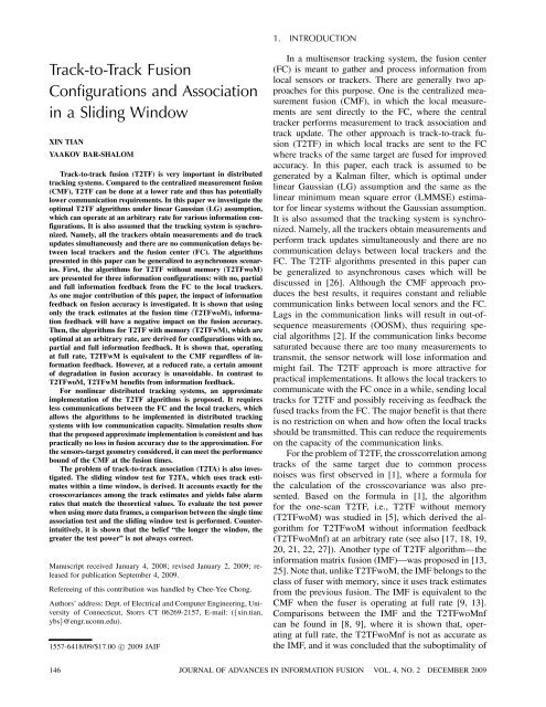
In a multisensor tracking system, the fusion center 

(FC) is meant to gather and process information from 

local sensors or trackers. There are generally two approaches 

for this purpose. One is the centralized measurement 

fusion (CMF), in which the local measurements 

are sent directly to the FC, where the central 

tracker performs measurement to track association and 

track update. The other approach is track-to-track fusion 

(T2TF) in which local tracks are sent to the FC 

where tracks of the same target are fused for improved 

accuracy. In this paper, each track is assumed to be 

generated by a Kalman filter, which is optimal under 

linear Gaussian (LG) assumption and the same as the 

linear minimum mean square error (LMMSE) estimator 

for linear systems without the Gaussian assumption. 

It is also assumed that the tracking system is synchronized. 

Namely, all the trackers obtain measurements and 

perform track updates simultaneously and there are no 

communication delays between local trackers and the 

FC. The T2TF algorithms presented in this paper can 

be generalized to asynchronous cases which will be 

discussed in [26]. Although the CMF approach produces 

the best results, it requires constant and reliable 

communication links between local senors and the FC. 

Lags in the communication links will result in out-ofsequence 

measurements (OOSM), thus requiring special 

algorithms [2]. If the communication links become 

saturated because there are too many measurements to 

transmit, the sensor network will lose information and 

might fail. The T2TF approach is more attractive for 

practical implementations. It allows the local trackers to 

communicate with the FC once in a while, sending local 

tracks for T2TF and possibly receiving as feedback the 

fused tracks from the FC. The major benefit is that there 

is no restriction on when and how often the local tracks 

should be transmitted. This can reduce the requirements 

on the capacity of the communication links. 

For the problem of T2TF, the crosscorrelation among 

tracks of the same target due to common process 

noises was first observed in [1], where a formula for 

the calculation of the crosscovariance was also presented. 

Based on the formula in [1], the algorithm 

for the one-scan T2TF, i.e., T2TF without memory 

(T2TFwoM) was studied in [5], which derived the algorithm 

for T2TFwoM without information feedback 

(T2TFwoMnf) at an arbitrary rate (see also [17, 18, 19, 

20, 21, 22, 27]). Another type of T2TF algorithm–the 

information matrix fusion (IMF)–was proposed in [13, 

25]. Note that, unlike T2TFwoM, the IMF belongs to the 

class of fuser with memory, since it uses track estimates 

from the previous fusion. The IMF is equivalent to the 

CMF when the fuser is operating at full rate [9, 13]. 

Comparisons between the IMF and the T2TFwoMnf 

can be found in [8, 9], where it is shown that, operating 

at full rate, the T2TFwoMnf is not as accurate as 

the IMF, and it was concluded that the suboptimality of 

146 JOURNAL OF ADVANCES IN INFORMATION FUSION VOL. 4, NO. 2 DECEMBER 2009

T2TFwoMnf is because it is optimal only in ML sense. 1 

However, the IMF is not optimal when the fuser is operating 

at reduced rate and, as reported in [10], it causes 

inconsistency and even divergence. A simulation based 

comparison on existing fusion algorithms can also be 

found in [23]. 

In this paper, the T2TF algorithms that can operate at 

an arbitrary rate are investigated for various information 

configurations: 

1. T2TFwoMnf (T2TFwoM with no information feedback) 

2. T2TFwoMpf (T2TFwoM with partial information 

feedback) 

3. T2TFwoMff (T2TFwoM with full information feedback) 

4. T2TFwMnf (T2TFwM with no information feedback) 

5. T2TFwMpf (T2TFwM with partial information feedback) 

6. T2TFwMff (T2TFwM with full information feedback) 

Except for T2TFwoMnf presented in [5], the results 

for all the other configurations are new. The impact of 

informationfeedbackandmemoryontheaccuracyof 

T2TF is thoroughly examined. 

For T2TFwoM, depending on the existence of information 

feedback, the three information configurations 

[6, 15] are illustrated in Fig. 1. Suppose there are two 

tracks (that pertain to the same target) which are fused at 

certain times. The first configuration is the T2TFwoM 

without information feedback (T2TFwoMnf) [3], designated 

as Type IIa configuration for multisensor trackingin[6].AsindicatedinFig.1(a),thetwolocaltracks 

evolve independently without the information from each 

other, thus the improved accuracies are achieved only 

at the fusion times at the FC. The second configuration 

is the T2TFwoM with partial information feedback 

(T2TFwoMpf) which belongs to the Type IIb configuration 

in [6]. In this case, as shown in Fig. 1(b), track 1 

is fused with track 2 and continues with the fused track 

(feedback) from the FC. However, track 2 does not receive 

the fused track in view of the partial information 

feedback. The third configuration is the T2TFwoM with 

full information feedback (T2TFwoMff), which also belongs 

to the Type IIb configuration in [6]. As shown in 

Fig. 1(c), both local trackers receive and continue with 

the fused track. 

As shown in this paper T2TFwoM has a degradation 

in fusion accuracy compared to the CMF, and information 

feedback has a negative impact on the fusion accuracy 

of T2TFwoM. However the degradation in fusion 

accuracy of T2TwoM can be recovered by using also the 

track estimates from the previous fusion. Accordingly, 

1 The actual reason that T2TFwoMnf is (slightly) inferior to IMF operating 

at full rate (when it is algebraically equivalent to CMF, see [6] 

Section 8.6) is the lack of memory of T2TwoMnf. This is discussed 

in detail in Section 2.4 and Section 3.4. 

Fig. 1. Information configurations for T2TFwoM (horizontal axis 

is time). (a) T2TFwoM with no feedback. (b) T2TFwoM with partial 

feedback (Fusion Center to Tracker 1). (c) T2TFwoM with full 

feedback (Fusion Center to Tracker 1 and Tracker 2). 

the algorithms for T2TFwM are derived for configurations 

with no, partial and full information feedback. It 

is shown that, when operating at full rate, T2TFwM is 

equivalent to the CMF (which is the global optimum) regardless 

of information feedback. However, at reduced 

rate, a certain amount of loss in fusion accuracy is unavoidable, 

and in contrast to the case of T2TFwoM, 

information feedback improves the fusion accuracy of 

T2TFwM. Furthermore, unlike the IMF, the T2TFwM 

algorithms derived in this paper are optimal at any rate. 

As pointed out in [8], the major difficulty for the 

practical implementation of the optimal T2TF algorithm 

is that it requires all the local filter gains and observation 

matrices since the last fusion. In nonlinear distributed 

tracking systems, the local information is not directly 

available at the FC. In view of this, we propose an approximate 

implementation of the T2TF algorithms. It is 

based on the idea of reconstructing local information 

at the FC with minimum amount of information from 

the local trackers, which has much less communication 

requirements than the transmission of those local matrices 

[12]. Simulation results show that this approximate 

implementation is consistent and has practically no loss 

in accuracy due to the approximation. 

Studies on the problem of track-to-track association 

(T2TA) can be found in [4, 24], in which the tests for 

T2TA are made based on a single frame of data. In 

[16], it is claimed that the test based on an average of 

TRACK-TO-TRACK FUSION CONFIGURATIONS AND ASSOCIATION IN A SLIDING WINDOW 147

TABLE I 

List of Acronyms 

CMF Centralized Measurement Fusion configuration IV 

IMF Information Matrix Fusion special configuration II M 

T2TF 

Track-to-Track Fusion 

T2TFwoM Track-to-Track Fusion without memory configuration II 

T2TFwoMnf T2TFwoM with no information feedback configuration II nf 

T2TFwoMpf T2TFwoM with partial information feedback configuration II pf 

T2TFwoMff T2TFwoM with full information feedback configuration II ff 

T2TFwM Track-to-Track Fusion with memory configuration II M 

T2TFwMnf T2TFwM with no information feedback configuration II M nf 

T2TFwMpf T2TFwM with partial information feedback configuration II M pf 

T2TFwMff T2TFwM with full information feedback configuration II M ff 

the single time tests within a time window has improved 

performance over the single time test. However, this 

conclusion was drawn ignoring the state errors’ crosscorrelation 

in time [7]. In this paper the chi-square based 

sliding window test for T2TA, which uses track estimates 

within a time window, is derived. It accounts exactly for 

all the crosscovariances among the track estimates and 

yields false alarm rates that match the theoretical values. 

To evaluate the test power when using more data frames 

(longer window), a comparison between the single time 

test and the sliding window test is performed. Counterintuitively, 

it is shown that the belief “the longer the 

window, the more the power” is not necessarily correct. 

This is because the power of the test depends on both the 

noncentrality parameter and the degrees of freedom of 

the (chi-square) test statistic. When the multiple frames 

of data selected for T2TA are strongly correlated, which 

happens for motion with low process noises (because 

the filter has “longer memory” in this case), the gain in 

the noncentrality parameter by using more data frames 

is too small to overcome the negative impact of the increased 

degrees of freedom on the power of the test. 

Thus, the sliding window test may be counterproductive 

and has lower power thanthesingletimetest. 

All the results presented are optimal under the LG 

assumption. 2 The paper is organized as follows. Section 

2 discusses the algorithms for T2TFwoM with no, 

partial and full information feedback. Section 3 derives 

the algorithms for T2TFwM with no, partial and full 

information feedback and shows the impact of information 

feedback on T2TFwM. In Section 4, the approximate 

implementation of the T2TF algorithms is proposed 

and evaluated in a tracking scenario with a nonlinear 

measurement model. The problem of T2TA test is 

investigated in Section 5, where the sliding window test 

is derived and compared with the single time test. Section 

6 summarizes the paper with conclusions. For the 

convenience of readers, Table I lists the acronyms used 

in this paper and extends the configurations discussed 

in [6]. 

2. TRACK-TO-TRACK FUSION WITHOUT MEMORY 

(T2TFwoM) AT AN ARBITRARY RATE 

2 In the case of fusion the algorithms presented constitute the LMMSE 

fuser, also called BLUE in, e.g., [18]. 

This section investigates the algorithms of 

T2TFwoM (configuration II [6]) at an arbitrary rate. 

Section 2.1 formulates the problem. In Section 2.2 

the T2TFwoM algorithms are presented for information 

configurations: with no, partial and full information 

feedback. Section 2.3 presents the simulation results 

that compare the fusion accuracies of T2TFwoMnf, 

T2TFwoMpf, T2TFwoMff and CMF. This leads to the 

observation that, in T2TFwoM, information feedback 

will cause a degradation of the fusion accuracy. This 

phenomenon is further explained in Section 2.4. 

2.1. Problem Formulation: T2TFwoM 

Consider the basic scenario with two local trackers 

(designated as 1 and 2) at different locations. Each 

tracker obtains measurements with its local sensor and 

maintains local tracks of the targets. For the sake of 

simplicity, it is assumed that the system operates in a 

synchronous fashion, where all the trackers obtain measurements 

and do local track updates simultaneously 

with sampling interval T. Communication links, which 

have no delay in time, are available between the FC and 

the local trackers. Each local tracker is allowed to communicate 

with the FC once in a while, sending its tracks 

to the FC and possibly receiving the fused tracks (when 

there is information feedback). At the FC, the fusion of 

the tracks of a target from trackers 1 and 2 is formulated 

as follows. 3 Let ˆx 1 (k j k), P 1 (k j k) andˆx 2 (k j k), P 2 (k j k) 

represent the two local tracks at the fusion time. Assuming 

the crosscovariance of the two tracks P 12 (k j k) 

is available at the FC, T2TFwoM should be performed, 

so that 

[ˆx c (k j k),P c (k j k)] 

= f[ˆx 1 (k j k),P 1 (k j k), ˆx 2 (k j k),P 2 (k j k),P 12 (k j k)] 

(1) 

where ˆx c (k j k)andP c (k j k) represent the fused track. After 

the fusion, the local tracks and their crosscovariance 

should also be updated to ˆx 

1 ¤ (k j k), P¤ 

1 (k j k), ˆx 

2 ¤ (k j k), 

3 Association (see [6] Section 8.4) is assumed to have been already 

performed. 


P 

2 ¤ 

(k j k) andP¤ 

12 

(k j k) according to the information configuration 

of the fusion (possible feedback from the FC). 

Throughout the paper, superscript “¤” is used to indicate 

post-fusion tracks. Note that (1) implies that only 

the local track estimates at the fusion time are used for 

T2TFwoM, i.e., this is a fuser without memory of fused 

and local track estimates from the previous fusion time. 4 

2.2. The Algorithms for T2TFwoM 

If the local tracks ˆx 1 (k j k), P 1 (k j k), ˆx 2 (k j k), P 2 (k j k) 

and their crosscovariance P 12 (k j k) are available at the 

FC, the optimal 5 T2TFwoM can be done according to 

Eqs. (8.4.4-4)—(8.4.4-5) in [6], namely, 

ˆx c (k j k)=ˆx 1 (k j k)+[P 1 (k j k) ¡ P 12 (k j k)] 

¢ [P 1 (k j k)+P 2 (k j k) ¡ P 12 (k j k) ¡ P 21 (k j k)] ¡1 

¢ [ˆx 2 (k j k) ¡ ˆx 1 (k j k)] 

= ˆx 1 (k j k)+K 12 (k)[ˆx 2 (k j k) ¡ ˆx 1 (k j k)] (2) 

P c (k j k)=P 1 (k j k) ¡ [P 1 (k j k) ¡ P 12 (k j k)] 

where 

¢ [P 1 (k j k)+P 2 (k j k) ¡ P 12 (k j k) ¡ P 21 (k j k)] ¡1 

¢ [P 1 (k j k) ¡ P 21 (k j k)] (3) 

P 12 (k j k)=P 21 (k j k) 0 =Cov[˜x 1 (k j k), ˜x 2 (k j k)]: (4) 

To calculate P 12 (k j k), suppose the previous fusion was 

performed at discretized time l, after which one has the 

errors 

˜x 1 ¤ (l j l)=ˆx 1 ¤ (l j l) ¡ x(l) (5) 

˜x 2 ¤ (l j l)=ˆx 2 ¤ (l j l) ¡ x(l) (6) 

where x(l) denotes the true state of the target at l. Let 

P 1 ¤ 1 ¤ (l j l), ˜x 1 ¤ (l j l)] (7) 

P 2 ¤ 2 ¤ (l j l), ˜x 2 ¤ (l j l)] (8) 

P 12 ¤ 1 ¤ (l j l), ˜x 2 ¤ (l j l)]: (9) 

From Eq. (8.4.2-2) in [6], one has 

˜x s (l +1j l +1)=[I ¡ K s (l +1)H s (l +1)]F(l)˜x s (l j l) 

¡ [I ¡ K s (l +1)H s (l +1)]v(l) 

+ K s (l +1)w s (l +1) s =1,2: 

(10) 

4 A fuser with memory (of the previous track estimates) uses the track 

estimates from the previous fusion time, which, as shown in Section 

3.4, improves fusion accuracy. 

5 MMSE if all the estimation errors are Gaussian and LMMSE otherwise 

[7]. 

Using (10) recursively for both the cental and local 

tracks from discrete time l to k, itfollowsthat 

kX 

˜x s (k j k)=Ws e (k,l)˜x s ¤ (l j l)+ 

+ 

kX 

i=l+1 

i=l+1 

where the weights are defined as 

k¡l¡1 

Ws e (k,l)= 

W v 

s 

and 

W w 

Ws v (k,i ¡ 1)v(i ¡ 1) 

Ws w (k,i)w s (i), s = 1,2 (11) 

Y 

[I ¡ K s (k ¡ i)H s (k ¡ i)]F(k ¡ i ¡ 1) 

i=0 

(12) 

(k,i ¡ 1) 

8 

9 

< k¡i¡1 

Y 

= 

= ¡ [I ¡ K 

: 

s (k ¡ j)H s (k ¡ j)]F(k ¡ j ¡ 1) 

; 

j=0 

¢ [I ¡ K s (i)H s (i)] (13) 

s (k,i) 

8 

9 

< k¡i¡1 

Y 

= 

= [I ¡ K 

: 

s (k ¡ j)H s (k ¡ j)]F(k ¡ j ¡ 1) 

; K s (i) 

j=0 

(14) 

in which K s (i), i = l +1,:::,k are the Kalman filter 

gains and H s (i) are the observation matrices at local 

tracker s and F(i ¡ 1) are the state transition matrices. 

Eq. (11) is the expression of the errors of the tracks 

from Kalman filters as weighted sums of the previous 

error at a certain point and the intervening process and 

measurement noises. The significance of this expression 

is that it shows explicitly all the sources of uncertainty 

and provides the general tool for the derivations of the 

T2TF and T2TA algorithms in the absence or presence 

of memory and feedback. 

From (11) and the whiteness assumption of the measurement 

noises and the process noises, the crosscovariance 

P 12 (k j k), required by the T2TFwoM given in 

(2)—(3), can be calculated as 

P 12 (k j k)=W1 e (k,l)P¤ 12 

kX 

+ 

i=l+1 

W v 

1 

(l j l)We 2 (k,l)0 

(k,i ¡ 1)Q(i ¡ 1)Wv 2 (k,i ¡ 1)0 

(15) 

where Q(i) is the covariance of the process noises at 

time i. Similarly to (11), the error of the fused track (2) 

can be expressed as 

˜x c (k j k)=˜x 1 (k j k)+K 12 (k)[˜x 2 (k j k) ¡ ˜x 1 (k j k)] 

=[I ¡ K 12 (k)]˜x 1 (k j k)+K 12 (k j k)˜x 2 (k j k): 

(16) 


After the fusion, local tracks 1 and 2 and their crosscovariance 

should be updated according to the information 

configuration. 

In configuration T2TFwoMnf (see Fig. 1(a)), one 

has 

ˆx ¤ 1 (k j k)=ˆx 1 (k j k) (17) 

P 1 ¤ 1 (k j k) (18) 

ˆx 2 ¤ (k j k)=ˆx 2 (k j k) (19) 

P 2 ¤ (k j k)=P 2 (k j k) (20) 

P 12 ¤ (k j k)=P 12 (k j k) (21) 

where P 12 (k j k) is given in (15). 

In configuration T2TFwoMpf (see Fig. 1(b)) 

ˆx ¤ 1 (k j k)=ˆx c (k j k) (22) 

P 1 ¤ c (k j k) (23) 

ˆx 2 ¤ (k j k)=ˆx 2 (k j k) (24) 

P 2 ¤ (k j k)=P 2 (k j k) (25) 

and according to (16) 

P ¤ 

12 (k j k)=[I ¡ K 12 (k)]P 12 (k j k)+K 12 (k)P 2 (k j k): (26) 

In configuration T2TFwoMff (see Fig. 1(c)) 

ˆx ¤ 2 (k j k)=ˆx ¤ 1 (k j k)=ˆx c (k j k) (27) 

P 2 ¤ (k j k)=P¤ 1 (k j k)=P c (k j k) (28) 

P 12 ¤ (k j k)=P c (k j k): (29) 

The algorithm of T2TFwoM is summarized as follows: 

² At the FC, the local tracks are fused according to 

(2)—(3). 

² The fusion can be done exactly, if the following data 

are available: 

(i) The local tracks to be fused: ˆx 1 (k j k), P 1 (k j k) and 

ˆx 2 (k j k), P 2 (k j k) 

(ii) The covariances and crosscovariance from the 

previous fusion at time l: P 

1 ¤ (l j l), P¤ 

2 

(l j l), P¤ 

12 (l j 

l) (see (7)—(8))–needed for the calculation of the 

current crosscovariance. 

(iii) The local weights (12)—(13). 

² Depending on the information configuration, the local 

tracks are updated accordingly using (17)—(21) for 

T2TFwoMnf, or (22)—(26) for T2TFwoMpf, or (27)— 

(29) for T2TFwoMff. 

The algorithm of T2TFwoM has no theoretical limit on 

the number of the local trackers. Only the crosscovariances 

among all the tracks of the same target need to be 

properly calculated. See [11] for the n-sensors version 

of the fusion equations (2)—(3). The use of the results 

from [11] in the general case requires Eqs. (11)—(13) 

for each sensor. 

TABLE II 

Fuser Variances (at fusion times) in Steady State 

(fusion interval: 5 s) 

Fusion Type 

FCTrackatFusionTime 

Pos 

Vel 

T2TFwoMff 133 6.29 

T2TFwoMpf 131 6.30 

T2TFwoMnf 125 6.30 

CMF 119 6.03 

2.3. Comparison of the T2TFwoM Algorithms and the 

CMF 

The algorithms for T2TFwoM are evaluated first in 

the following tracking scenario. The target state is defined 

as [x _x] 0 . The target motion is modeled as the 

discrete white noise acceleration (DWNA) model in [7], 

Section 6.3.2. It is assumed that two sensors obtain position 

measurements of the target with a sampling interval 

of T = 1 s. The standard deviation of the measurement 

noise is ¾ w = 30 m and the process noise variance is 

q =1m 2 =s 4 . T2TFwoM takes place every 5 s, i.e., at a 

reduced rate. 

All the fusers are consistent in the simulations (their 

covariance calculations are exact). In view of the consistency, 

the performance comparison can be made using 

the calculated covariances. Table II shows the steady 

state variances of position and velocity at the FC. All 

the fused tracks are more accurate than the single-sensor 

(local) tracks without fusion, which have steady state 

variances as 205 in position and 7.26 in velocity. Note 

that at the fusion time the position estimates of all 

the fused tracks have a small degradation compared to 

the CMF: 5% for T2TFwoMnf, 10% for T2TFwoMpf, 

12% for T2TFwoMff. This shows that T2TFwoM has 

a degradation in fusion accuracy compared to the CMF 

and the degradation increases in the presence of information 

feedback. This apparently counterintuitive result 

is further discussed in the next subsection. 

2.4. The Impact of Information Feedback on 

T2TFwoM 

To show the impact of information feedback on 

T2TFwoM, consider the following two-step scalar estimation 

problem. At time 0, two local estimators have 

independent prior information: ¯x 1 » N(x(0),P 1 )atestimator 

1 and ¯x 2 » N(x(0),P 2 ) at estimator 2. At time 1, 

x(1) = x(0) + v 1 where the process noise v 1 » N(0,Q). 

The estimators have independent measurements of the 

state: z 1 = x(1) + w 1 (w 1 » N(0,R 1 )) at estimator 1 and 

z 2 = x(1) + w 2 (w 2 » N(0,R 2 )) at estimator 2. The errors 

in the prior information, the process noise and the measurement 

noises are all independent. For the sake of simplicityitisassumedthatP 

1 = P 2 = R 1 = R 2 =1andQ = 

1=2. Consider the fusion at time 1 and the fuser uses 

only the track estimates at time 1, namely T2TFwoM. 

Fig. 2 shows the information flow of the centralized 



Cov[ˆx ff (1 j 1)] = 3 8 : (35) 

In T2TFwoMnf (Configuration IIa in Section 8.2.3 

[6]), it follows that 

ˆx nf (1 j 1) = 1 ¯x 5 1 + 1 ¯x 5 2 + 3 10 z 1 + 3 

10 z 2 (36) 

with error 

˜x nf (1 j 1) = 1 ˜x 5 1 + 1 ˜x 5 2 ¡ 2 5 v 1 + 3 10 w 1 + 3 10 w 2 (37) 


Then one has 

Cov[ˆx nf (1 j 1)] = 17 

50 : (38) 

Cov[ˆx CMF (1 j 1)] < Cov[ˆx nf (1 j 1)] < Cov[ˆx ff (1 j 1)]: 

(39) 

There are losses in accuracy in T2TFwoMff and 

T2TFwoMnf compared to the CMF, although they are 

relatively small, due to the large process noise in the 

example. Comparing (31), (34) and (37), it can be 

seen that the weights of the measurements are lower 

in T2TFwoMnf than in the CMF. They become even 

lower in T2TFwoMff due to the information feedback, 

which leads to the further loss in fusion accuracy. 

Fig. 2. Information flow (CMF and T2TFwoM). (a) CMF 

(configuration IV). (b) T2TFwoMff (configuration IIff). 

(c) T2TFwoMnf (configuration IInf). 

measurement fusion (CMF), T2TFwoM with full information 

feedback (T2TFwoMff) and T2TFwoM with 

no information feedback (T2TFwoMnf). Note that in 

T2TFwoMff the information feedback (sharing) occurs 

attime0inthisexample. 

Using CMF (Configuration IV in Section 8.2.5 of 

[6]), one has 

ˆx CMF (1 j 1) = 1 6 ¯x 1 + 1 6 ¯x 2 + 1 3 z 1 + 1 3 z 2 (30) 

with error (using the weighted sum form) 

˜x CMF (1 j 1) = 1 6 ˜x 1 + 1 6 ˜x 2 ¡ 1 3 v 1 + 1 3 w 1 + 1 3 w 2 (31) 

where ˜x 1 and ˜x 2 denote the errors of ¯x 1 and ¯x 2 .Itiseasy 

to calculate the covariance 

In T2TFwoMff, 6 one has 

with error 

Cov[ˆx CMF (1 j 1)] = 1 3 : (32) 

ˆx ff (1 j 1) = 1 4 ¯x 1 + 1 4 ¯x 2 + 1 4 z 1 + 1 4 z 2 (33) 

˜x ff (1 j 1) = 1 4 ˜x 1 + 1 4 ˜x 2 ¡ 1 2 v 1 + 1 4 w 1 + 1 4 w 2 (34) 

6 Note that, following Section 8.2.3 of [6], Configuration IIb does not 

have a memory of past estimates at the FC. It is T2TFwoM. 

3. THE ALGORITHMS FOR T2TFwM AT AN 

ARBITRARY RATE 

The results in Section 2.4 show that, at full rate, 

T2TFwoM is less accurate than the CMF and information 

feedback is detrimental to T2TFwoM. However, the 

IMF is equivalent to the CMF when operating at full 

rate [13]. In this case, T2TFwoM is inferior to the IMF. 

This is because T2TFwoM uses only local estimates at 

the fusion time, which contain most but not all of the 

information for T2TF. In contrast, the IMF belongs to 

theclassofT2TFwM.However,atreduced rate, the 

IMF algorithm is not optimal anymore. 

To account for the information from the fused and 

local track estimates from the previous fusion time, 7 the 

algorithm for T2TFwM at an arbitrary rate is derived 

in the next three subsections for configurations with 

no, partial and full information feedback, designated as 

T2TFwMnf, T2TFwMpf and T2TFwMff respectively. 

Fig. 3 shows the information flow of the three configurations. 

3.1. The Algorithm for T2TFwMnf 

As shown in Fig. 3(a), for T2TFwMnf, at fusion 

time k, the track estimates to be fused are local track 

7 This implies one-step memory. In fact, there is no need for more, 

since one-step memory summarizes, under the LG (or LMMSE) assumptions, 

all the information from the previous track estimates. This 

is confirmed by the simulation results in Section 3.4, which show that, 

at full rate, T2TFwM (using one-step memory) yields the globally optimal 

fusion results. 


Fig. 3. Information flow: T2TFwM at an arbitrary rate. (a) T2TFwM with no information feedback (one cycle: from fusion time l to 

the next fusion time k). (b) T2TFwM with partial information feedback (one cycle: from fusion time l to the next fusion time k). 

(c) T2TFwM with full information feedback (one cycle: form fusion time l to the next fusion time k). 

estimates ˆx 1 (k j k), ˆx 2 (k j k) and the predicted track estimates 

ˆx 1 (k j l), ˆx 2 (k j l) andˆx c (k j l) from the previous 

fusion, where subscript “c” indicates the (fused) track 

at the FC. Stacking the estimates and the predicted estimates 

as a vector, one has 

¹ =[ˆx 1 (k j k) ˆx 2 (k j k) ˆx c (k j l) ˆx 1 (k j l) ˆx 2 (k j l)] 0 : 

(40) 

The fusion of these track estimates requires the covariance 

of ¹, denoted as Cov(¹). To obtain this covariance, 

a slight modification of (11) gives 

˜x s (k j l)=W e 

0 (k,l)˜x ¤ s (l j l)+ kX 

where s =1,2,c and 

W v 

Y 

k¡l¡1 

W0 e (k,l)= 

i=0 

i=l+1 

W0 v (k,i ¡ 1)v(i ¡ 1) 

(41) 

F(k ¡ i ¡ 1) (42) 

k¡i¡1 

0 (k,i ¡ 1) = ¡ Y 

F(k ¡ j ¡ 1) (43) 

j=0 

which are obtained by substituting the filter gains K s (i) 

in (12) and (13) by zero matrices, since the filter gains 

are zero in the predicted track estimates. From (12), 

(13), (42) and (43), Cov(¹) can be easily calculated with 

linear algebra. 

For T2TFwMnf, define the following difference matrix 

2 

3 

I 0 ¡I 0 0 

0 I ¡I 0 0 

M = 6 

7 (44) 

40 0 ¡I I 05 

0 0 ¡I 0 I 

where I denotes identity matrix of appropriate dimension, 

such that 

2 

3 

ˆx 1 (k j k) ¡ ˆx c (k j l) 

ˆx 2 (k j k) ¡ ˆx c (k j l) 

º = 

= M¹: (45) 

6 

4 

ˆx 1 (k j l) ¡ ˆx c (k j l) 7 

5 

ˆx 2 (k j l) ¡ ˆx c (k j l) 

Using the standard MMSE estimator from [7], the fused 

estimate is given by 

ˆx c (k j k)=ˆx c (k j l)+Cov[x(k),º]Cov(º) ¡1 º (46) 

where x(k) is the true state of the target at time k, and 

Cov[x(k),º]=¡[Cov(¹)] (3,:) M 0 (47) 

Cov(º)=MCov(¹)M 0 (48) 

where [Cov(¹)] (i,:) denotes the ith row of matrix Cov(¹). 

In (46) ˆx c (k j l) plays the role of the prior at the FC and 

the other elements of ¹ play the role of the observations. 


From (45)—(48), the fused estimate is 

ˆx c (k j k)=ˆx c (k j l) ¡ [Cov(¹)] (3,:) M 0 (MCov(¹)M 0 ) ¡1 M¹ 

where 

= ˆx c (k j l)+K ¹ ¹ (49) 

K ¹ 

¢ 

=¡[Cov(¹)](3,:) M 0 (MCov(¹)M 0 ) ¡1 M: (50) 

The fused covariance is 

P c (k j k)=P c (k j l) ¡ Cov[x(k),º]Cov(º) ¡1 Cov[x(k),º] 0 

= P c (k j l) ¡ [Cov(¹)] (3,:) M 0 (MCov(¹)M 0 ) ¡1 M 

¢ [[Cov(¹)] (3,:) ] 0 

= P c (k j l)+K ¹ [[Cov(¹)] (3,:) ] 0 : (51) 

For T2TFwMnf the crosscovariances between the fused 

track and the tracks from trackers 1 and 2 can be 

obtained from (49) as 

P 1c (k j k) ¢ =Cov[ˆx 1 (k j k), ˆx c (k j k)] 

=[Cov(¹)] (1,3) +[Cov(¹)] (1,:) K 0 ¹ (52) 

P 2c (k j k) ¢ =Cov[ˆx 2 (k j k), ˆx c (k j k)] 

=[Cov(¹)] (2,3) +[Cov(¹)] (2,:) K¹ 0 (53) 

where [Cov(¹)] (i,j) is element (i,j) ofCov(¹). 

Since there is no information feedback, both local 

tracks are not changed after the fusion is performed at 

theFC.Onehas 

ˆx 1 ¤ (k j k)=ˆx 1 (k j k) (54) 

P 1 ¤ 1 (k j k) (55) 

ˆx 2 ¤ (k j k)=ˆx 2 (k j k) (56) 

P 2 ¤ 2 (k j k) (57) 

P 12 ¤ 12 (k j k) (58) 

P 1c ¤ 1c (k j k) (59) 

P 2c ¤ 2c (k j k): (60) 

3.2. The Algorithm for T2TFwMpf 

Unlike T2TFwMnf, in T2TFwMpf, one has 

ˆx 1 (k j l)=ˆx c (k j l). Consequently, the elements ˆx 1 (k j l) 

in (40) should be removed. In this case, redefine ¹ in 

(40) and M in (44) as 

¹ =[ˆx 1 (k j k) ˆx 2 (k j k) ˆx c (k j l) ˆx 2 (k j l)] 0 (61) 


2 

I 0 ¡I 

3 

0 

M = 

¢ 6 

40 I ¡I 

7 

05: (62) 

0 0 ¡I I 

It follows that 

2 

3 

ˆx 1 (k j k) ¡ ˆx c (k j l) 

6 

7 

º = 4 ˆx 2 (k j k) ¡ ˆx c (k j l) 5 = M¹: (63) 

ˆx 2 (k j l) ¡ ˆx c (k j l) 

Then, similarly to T2TFwMnf, the fused estimate 

ˆx c (k j k) is obtained using (49) and the fused covariance 

P c (k j k) follows from (51) using the modified definitions 

(61) and (62). 

After the fusion, the local tracks and the track crosscovariances 

are updated as follows 

ˆx ¤ 1 (k j k)=ˆx c (k j k) (feedback) (64) 

P 1 ¤ c (k j k) (feedback) (65) 

P 1c ¤ c (k j k) (feedback) (66) 

ˆx 2 ¤ (k j k)=ˆx 2 (k j k) (no feedback) (67) 

P 2 ¤ 2 (k j k) (no feedback) (68) 

P 12 ¤ 2c (k j k)0 (69) 

P 2c ¤ 2c (k j k) (70) 

where P 2c (k j k) is given by (53) using the modified 

definitions (61) and (62). 

3.3. The Algorithm for T2TFwMff 

In contrast to T2TFwMnf, in T2TFwMff, one has 

ˆx 1 (k j l)=ˆx 2 (k j l)=ˆx c (k j l). Consequently, the elements 

ˆx 1 (k j l) andˆx 2 (k j l) in (40) should be removed. In this 

case, redefine ¹ in (40) and M in (44) as 


¹ =[ˆx 1 (k j k) ˆx 2 (k j k) ˆx c (k j l)] 0 (71) 

· ¸ I 0 ¡I 

M = 

: (72) 

0 I ¡I 


· ¸ 

ˆx 1 (k j k) ¡ ˆx c (k j l) 

º = 

= M¹: (73) 

ˆx 2 (k j k) ¡ ˆx c (k j l) 

Then, similarly to T2TFwMnf, the fused estimate is 

obtained using (49) and the fused covariance follows 

from (51) using the modified definitions (71) and (72). 

Due to full information feedback, the local tracks 

and the track crosscovariances are updated as 

ˆx ¤ 1 (k j k)=ˆx c (k j k) (feedback) (74) 

P 1 ¤ c (k j k) (feedback) (75) 

P 1c ¤ c (k j k) (feedback) (76) 

ˆx 2 ¤ (k j k)=ˆx c (k j k) (feedback) (77) 

P 2 ¤ (k j k)=P 2 (k j k) (feedback) (78) 

P 12 ¤ (k j k)=P¤ 2c (k j k)=P c (k j k) (feedback): (79) 

Note that in T2TFwMff the crosscovariances between 

the fused track and the local tracks after the information 

feedback are the same with the fused covariance 

(51). This is different from the updated crosscovariances 

in T2TFwMnf, i.e., (59) and (60). 


TABLE III 

Fuser and Tracker 1 Calculated Variances at Fusion Times for N f =1(fullrate),q =0:3, R 1 = R 2 =1 

Time 1 2 3 4 5 6 

T2TFwMnf Tracker 1 1.0000 0.5652 0.4639 0.4331 0.4230 0.4196 

Fuser 0.5000 0.3077 0.2743 0.2673 0.2658 0.2654 

T2TFwMpf Fuser 0.5000 0.3077 0.2743 0.2673 0.2658 0.2654 

T2TFwMff Fuser 0.5000 0.3077 0.2743 0.2673 0.2658 0.2654 

CMF 0.5000 0.3077 0.2743 0.2673 0.2658 0.2654 

TABLE IV 

Fuser and Tracker 1 Calculated Variances at Fusion Times for N f = 3 (reduced rate), q =0:3, R 1 = R 2 =1 

Time 1 3 6 9 12 15 

T2TFwMnf Tracker1 1.0000 0.4639 0.4196 0.4180 0.4179 0.4179 

Fuser 0.5000 0.2772 0.2698 0.2694 0.2694 0.2694 

T2TFwMpf Fuser 0.5000 0.2763 0.2690 0.2688 0.2688 0.2688 

T2TFwMff Fuser 0.5000 0.2755 0.2683 0.2682 0.2682 0.2682 

CMF 0.5000 0.2743 0.2654 0.2653 0.2653 0.2653 

3.4. Performance Comparison: T2TFwMnf vs. 

T2TFwMff and CMF 

To evaluate the performance of the optimal T2TF 

with memory (T2TFwM) at an arbitrary rate, consider 

the following tracking scenario. The state of the target 

(taken as a scalar for simplicity) evolves according 

to 

x(k)=x(k ¡ 1) + v(k), k =2,3,::: (80) 

where v(k) is the process noise with variance q. 

There are two trackers, 1 and 2, taking measurements 

of the target with measurement noises w 1 and 

w 2 ,namely, 

z i (k)=x(k)+w i (k), i = 1,2 (81) 

where w i (k) are zero-mean Gaussian noises with variance 

R i . The two trackers calculate tracks of the target 

with their own measurements using a Kalman filter. 

Each local track is initialized at time 1 with the first 

local measurement. The first T2TF happens at time 1. 

Then T2TFwM occurs every N f sampling times. 

Table III shows the fuser- and tracker-calculated 

variances of the errors of the track estimates when the 

fuser is operating at full rate. It can be seen that, at full 

rate, the fuser with memory (with no, partial and full 

information feedback) is equivalent to the CMF. 

Table IV shows the fuser- and tracker-calculated 

variances when the fuser (with memory) is operating 

at reduced rate. In this case, T2TFwM, with or without 

information feedback, has a small loss in fusion accuracy 

compared to the CMF. This is because, in T2TF, 

information from the common process noises and the 

common prior information (due to information feedback) 

appears simultaneously in different local tracks, 

which causes their weights (and, consequently, also the 

weights of the new measurements) in the fused track 

to deviate from the global optimum. This is similar to 

the T2TFwoM example discussed in Section 2.4. When 

T2TFwM is done at full rate, these deviations are fully 

corrected by fusing the previous track estimates (see [6], 

Section 8.6). However, at a lower rate, the deviations can 

not be fully corrected, thus, a certain amount of degradation 

in fusion accuracy is unavoidable. Also note 

that, in contrast to the case of T2TFwoM, T2TFwMff 

is more accurate than T2TFwMpf and T2TFwMnf, 

namely information feedback improves fusion accuracy 

in T2TFwM (as expected). While it is too involved to 

provide a theoretical proof of this result, simulations in 

different settings confirm this. 

Another fusion algorithm that also uses the previous 

track estimates (i.e., it has memory) is the IMF [13, 25]. 

When operating at full rate, the IMF is algebraically 

equivalent to the CMF (see [6], Section 8.6) and also to 

the algorithms for T2TFwM presented in this section. 

However, at a lower rate, the IMF is not an optimal 

algorithm. As reported in [10], this may even lead to 

divergence. In contrast, the algorithms for T2TFwMnf, 

T2TFwMpf and T2TFwMff are optimal at any rate. 

3.5. Summary of the Various T2TF Configurations 

To summarize the discussion in Section 2 and Section 

3: 

² For T2TFwoM (which uses only the track estimates 

at the fusion time), information feedback will cause a 

degradation in fusion accuracy (see Section 2.4). This 

is because the local trackers use locally optimal but 

globally suboptimal filter gains, which leads to lower 

gains for the new measurements in the fused track. 


TABLE V 

Data Required from Local Tracker 2 for each Fusion with Fusion Interval of M 

Exact algorithm 

Data Required 

The Total Amounts (bits) 

W2 e (k,l), Wv 

2 (k,i ¡ 1), ˆx 2 , P 2 [(M +1)n 2 x + n x +0:5(n x +1)n x ]n acc 

Approximate Measurement time stamps, Mn T +[n x +0:5(n x +1)n x ]n acc 

algorithm ˆx 2 , P 2 

n acc : The number of the bits for each element in the state and covariance (accuracy) 

n x : Dimension of the state n T : The number of bits for each measurement time stamp 

Information feedback will lower the gains further, and 

cause more degradation in fusion accuracy. 

² The algorithms for T2TFwM (which uses also the 

track estimates from the previous fusion) at an arbitrary 

rate for different information configurations 

(with and without information feedback) are derived 

for the first time. When operating at full 

rate, T2TFwM, with no, partial or full information 

feedback, is equivalent to the CMF (global optimum). 

When operating at a reduced rate, T2TFwMnf, 

T2TFwMpf and T2TFwMff all have a small degradation 

in fusion accuracy compared to the CMF. However, 

unlike the case of T2TFwoM, the degradation 

is smaller for T2TFwMff than for T2TFwMpf and 

T2TFwMnf. Namely information feedback improves 

fusion accuracy in T2TFwM. 

4. THE APPROXIMATE IMPLEMENTATION OF THE 

T2TF ALGORITHMS 

The T2TF algorithms at an arbitrary rate require the 

local weight matrices (12)—(13) at the FC. However, 

transmission of these matrices might not be affordable 

in practical distributed tracking systems due to limit in 

communication capacity. The idea of the approximate 

implementation is to approximately reconstruct the local 

information required by the T2TF algorithms at the FC 

using a minimum amount of information from the local 

trackers. Section 4.1 presents the approximate implementation 

which has significantly lower communication 

requirements than the original algorithms. Simulation 

results in Section 4.2 show that this implementation is 

consistent and has practically no loss in the fusion accuracy 

due to the approximation. 

4.1. The Approximate Algorithm 

Note that the local weighting matrices (12)—(13) are 

functions of F(i ¡ 1), H s (i), K s (i), i = l +1,:::,k. Atthe 

FC, if estimates of the target positions (i.e., an approximate 

trajectory of the target) are available, using also 

the locations of the local sensors and the times when 

the local measurements are taken, the observation matrices 

used by the local tracker and the related track 

updates can be approximately reconstructed, yielding 

¯H s (i), ¯Ks (i), i = l +1,:::,k. Note that these reconstructions 

do not need the actual measurements due to the 

nature of the Kalman filter that the covariance updates 

do not depend on the actual measurements. Thus the 

approximate evaluation of (12)—(13) is given by 8 

¯W e 

s (k,l)= k¡l¡1 

Y 

[I ¡ ¯K s 

(k ¡ i) ¯H s 

(k ¡ i)]F(k ¡ i ¡ 1) (82) 

i=0 

( k¡i¡1 

) 

Y 

¯W v 

s (k,i ¡ 1) = ¡ [I ¡ ¯K s 

(k ¡ j) ¯H s 

(k ¡ j)]F(k ¡ j ¡ 1) 

j=0 

¢ [I ¡ ¯K s 

(i) ¯H s 

(i)] (83) 

where overbar denotes the approximate values. For 

T2TF, (15) can be approximated by 

¯P 12 (k j k)= ¯W 1 e (k,l)P¤ 12 

kX 

+ 

i=l+1 

(l j l) ¯W 

e 

2 (k,l)0 

¯W 1 v 

v 

(k,i ¡ 1)Q(i ¡ 1) ¯W 2 (k,i ¡ 1)0 : 

(84) 

Thus, to approximately calculate the local weights 

(12)—(13) required in the T2TF algorithms, the FC 

needs to know the following: (i) the locations of the 

local sensors, (ii) the time when the local measurements 

are obtained (considering the possibility of missed detections 

in practical systems) and (iii) an approximate 

trajectory of the target. Note that, at the FC, (iii) is available 

when there is a tracker running at the FC or it can 

be obtained by interpolation between the track estimates 

at the fusion times. Although extra computations are required 

at the FC to obtain the approximate weights at 

the local trackers, these computations are affordable due 

to the simplicity of the expressions involved. A brief 

analysis of the savings in communication is given below. 

In distributed tracking systems with sensors at fixed 

locations, there is no need to transmit the locations. Assume 

further that tracker 1 is collocated with the FC 

and, thus, the approximate track trajectory can be obtained 

from its track estimates. Table V compares the 

amount of data that needs to be transmitted from local 

tracker 2 to the FC in the exact algorithm and in 

8 If the measurements are linear (as in [18]) there is no need for this 

approximation. In the problem considered later, the measurements are 

nonlinear (range and azimuth); consequently, this approximation will 

be needed. 


Fig. 4. 

Filter consistency test: NEES (T2TFwoMff). 

Fig. 5. 

RMS position errors (T2TFwoMff). 

the approximate implementation. Given that transmission 

of measurement time stamps is much less expensive 

than transmission of the local weights, namely, 

(M +1)n 2 x n acc À Mn T , the savings in communication 

using the approximate algorithm is significant. 

4.2. Simulation Results 

The approximate implementation of the T2TF algorithms 

is tested in a 2-D multisensor tracking scenario, 

in which one target is tracked by two trackers. 

The target motion is modeled as a DWNA process [7] 

with process noise variance q. The target state is defined 

as x =[» _ » ³ _ ³] 0 . Tracker 1 is located at [0 0] m and 

tracker 2 is at [0 10000] m. The local sensors (radars) 

obtain position measurements of the target in their polar 

coordinates, namely, range and azimuth, every T =1s. 

The filter used by the trackers is the converted measurement 

Kalman filter (CMKF) [7]. It is assumed that 

tracker 1 is collocated with the FC, i.e., the FC has access 

to the estimates of tracker 1, and tracker 2 sends 

its track (ˆx 2 (k j k), P 2 (k j k)) to the FC every 10 sampling 

intervals. The simulation results are obtained from 100 

Monte-Carlo (MC) runs. 

4.2.1. T2TFwoM with full Information Feedback 

(T2TFwoMff) 

Figs. 4—5 show the performance of the approximate 

implementation in the case of T2TFwoMff. As 

shown in Fig. 4, the fused tracks are always consistent 

(the normalized estimation error squared (NEES)) 

are in their 95% probability region [3:46 4:69]). In 

Fig. 5, significant improvement in track accuracies 

from both trackers is observed at the fusion times 

k = 10,20,:::,100. The results of the CMF are also 

presented as the bound of the tracking performance. 

The root mean square (RMS) position errors indicate 

that the fused track practically meets the performance 

bound of the CMF at the fusion times. Between the 

fusion times the errors increase because each tracker 

is on its own. The loss of accuracy because of the 

information feedback in the fused track (discussed in 

Section 2.3) becomes insignificant due to the geometric 

diversity of the two tracks. 9 The results for velocity 

are similar. Since the approximate implementation 

performs practically as well as the CMF, there is no 

need in this case to evaluate the exact algorithm for 

T2TFwoMff. 

4.2.2. T2TFwoM with Partial Information Feedback 

(T2TFwoMpf) 

Figs. 6—7 show the performance of the approximate 

implementation in the case of T2TFwoMpf for the 

same tracking scenario with the following modification: 

tracker 2 does not receive the fused track from the FC. 

Fig. 6 shows that the fused track is consistent. In terms 

of achieved accuracy, it also meets the performance 

bound of the CMF at the fusion points. 

4.2.3. The Effect of Ignoring the Crosscovariance in 

T2TFwoMff 

Figs. 8—9 show the statistics from the same tracking 

scenario, but the T2TFwoMff is performed assuming 

that the two tracks are uncorrelated. The divergence 

of the filter–very rapid in NEES, slower but 

noticeable in RMSE–demonstrates the importance of 

taking into account the crosscovariances. This happens 

because the excessive optimism (fused covariances 

that are too small) due to ignoring the crosscovariances. 

9 With the two sensors widely separated (10000 m apart in the simulation), 

and the measurements much more accurate in the range direction 

than the crossrange direction, the two tracks are geometrically complementary 

to each other in the scenario considered. In such cases, 

the improvements of accuracy of the fused track are very significant, 

and they are less affected by the crosscorrelation between the tracks. 


Fig. 6. 

Filter consistency test: NEES (T2TFwoMpf). 

Fig. 8. Filter consistency test: NEES (T2TFwoMff). Ignoring the 

crosscovariances in T2TFwoMff leads to divergence. 

Fig. 7. 

RMS position errors (T2TFwoMpf). 

5. SLIDING WINDOW TEST FOR T2TA 

The chi-square based track-to-track association 

(T2TA) test is investigated in this section. Note that the 

chi-square based T2TA test is based only on the likelihood 

function (LF) under H 0 (the two tracks belong to 

the same target). The optimal (likelihood ratio–LR) test 

can not be used for T2TA, since the exact LF under H 1 

(the two tracks do not belong to the same target) is not 

available. Although a diffuse prior may be used to calculate 

the LF under H 1 , which leads to a LR test that is the 

same as the chi-square based test. The test still has virtually 

no information about H 1 . 10 The test can be done 

based on a single frame of track estimates, or using track 

estimates at multiple times. Conventional belief is that, 

given the same false alarm rate, using multiple frames 

of data will yield higher power. Accordingly the sliding 

window test is proposed in Section 5.1, which is shown 

10 Also note that the chi-square based test uses only the Gaussian 

exponent (This has the disadvantage that large covariance leads to 

acceptance but it has low power). The assignment, however, will use 

the full LF, i.e., there is penalty for large covariance matrix. 

Fig. 9. 

RMS position errors (T2TFwoMff). 

to yield false alarm rates that match the theoretical values. 

Then we compare the power of the sliding window 

test to that of the single time test. Counterintuitively, 

it is observed that the sliding window test, which uses 

more data, does not necessarily have more power than 

the single time test. The reason for this phenomenon is 

discussed in Section 5.2. 

5.1. The Algorithm of the Sliding Window Test for 

T2TA 

Consider the basic T2TA test of whether two tracks 

originated from the same target. For the single time test 

at time k, the data includes the tracks ˆx 1 (k j k), P 1 (k j k) 

from tracker 1 and ˆx 2 (k j k), P 2 (k j k) from tracker 2, as 

well as their crosscovariance P 12 (k j k). Define 

¢(k)=ˆx 1 (k j k) ¡ ˆx 2 (k j k): (85) 


P ¢ (k)=P 1 (k j k)+P 2 (k j k) ¡ P 12 (k j k) ¡ P 12 (k j k) 0 (86) 


where P 12 (k j k) is calculated from (15). The test statistic 

is 

T(k)=¢(k) 0 P ¢ (k) ¡1 ¢(k) (87) 

which, under H 0 (the two tracks are for the same target), 

is a random variable with a Â 2 n x 

distribution (n x is the 

dimension of the state). However, for data association at 

subsequent times, similar test statistics T(g), g>k,are 

correlated with T(k), thus the sum of single time test 

statistics (87) within a time window does not have a Â 2 

distribution [4, 24]. 11 

The sliding window test based on the most recent N 

frames of data needs to account for the crosscovariances 

among data at different times. Without loss of generality, 

consider the T2TA that occurs at time t m .Define 

¢ N (t m )=[¢(t m ) ¢(t m¡1 ):::¢(t m¡N+1 )] 0 (88) 

where subscript N is the window length and ¢(t m ),:::, 

¢(t m¡N+1 )arefromtheN most recent track estimates 

received by the FC. The test statistic T N (t m ) for this 

sliding window of N times is 

T N (t m )=¢ N (t m ) 0 Cov[¢ N (t m )] ¡1 ¢ N (t m ) (89) 

which, under H 0 ,hasaÂ 2 distribution with Nn x degrees 

of freedom. 

Given Cov[¢ N (t m¡1 )] from the previous sliding window, 

to obtain Cov[¢ N (t m )], the new diagonal term 

Cov[¢(t m )] = P ¢ (t m ) (90) 

is calculated from (86). The new off-diagonal terms are 

Cov[¢(t m 

),¢(t i 

)] 

=Cov[˜x 1 

(t m 

j t m 

) ¡ ˜x 2 

(t m 

j t m 

), ˜x 1 

(t i 

j t i 

) ¡ ˜x 2 

(t i 

j t i 

)] 

=Cov[˜x 1 

(t m 

j t m 

), ˜x 1 

(t i 

j t i 

)] + Cov[˜x 2 

(t m 

j t m 

), ˜x 2 

(t i 

j t i 

)] 

¡ Cov[˜x 1 

(t m 

j t m 

), ˜x 2 

(t i 

j t i 

)] ¡ Cov[˜x 2 

(t m 

j t m 

), ˜x 1 

(t i 

j t i 

)], 

i = m ¡ N +1,:::,m ¡ 1: (91) 

From (11), it follows that 

Cov[¢(t m 

),¢(t i 

)] = W 1 

e (t m ,t i )P 1 (t i j t i )+W2 e (t m ,t i )P 2 (t i j t i ) 

¡ W 1 

e (t m ,t i )P 12 (t i j t i ) ¡ W2 e (t m ,t i )P 21 (t i j t i ) 

(92) 

where P 1 (t i j t i ), P 2 (t i j t i ) are from the tracks at time t i 

and P 12 (t i j t i ) is calculated using (15). 

5.2. The Sliding Window Test vs. the Single Time Test 

The sliding window test using test statistics (89) and 

the single time test with test statistics (87) are compared 

in a 1-D multisensor tracking scenario as in Section 2.3. 

Target 1 starts at 5000 m with an initial velocity ¡3 m/s. 

Target 2 starts at 5030 m with the same initial velocity 

11 This is contrary to the assertion in [16]. 

Fig. 10. Miss probability (wrong rejection) from 100 MC runs for 

0.025 theoretical value (associations are done every 3 s). 

(the initial target separation is 30 m). 12 Both targets 

have process noises with variance q =2¢ 10 ¡2 m 2 =s 4 . 

These noises are independent across the targets, leading 

to their eventual separation. Two sensors, designated 

as 1 and 2, obtain position measurements of targets 1 

and2every1sandmaintainseparatetracksforthe 

targets. The T2TA tests are performed every 3 s, which 

is the time interval between two consecutive local track 

estimates used in the window test. The sliding window 

test uses a window of N = 5 times. For comparison, 

two tests based on the sum of the single time tests are 

also performed. One is the cumulative sum over all the 

previous single time tests; another is the sum of the 

single time tests within a sliding window of N as the 

approach proposed in [16, 24]. Both are not optimal 

because the correlations in time are ignored. 

Fig. 10 shows the miss probability when the track 

of target 1 at sensor 1 is associated with the track of the 

same target at sensor 2. The theoretical miss probability 

is 2.5% (correct acceptance 97.5%). The “single time 

test” (based on single frame of data) and the “sliding 

window test” match the theoretical error probability. 

However, the miss probabilities of the other two tests 

based on the sum of the single time test statistics are 

significantly larger than the theoretical value. This is 

due to the fact that these tests ignore the correlation 

among the single time test statistics. 

Fig. 11 shows the probability of correct rejection 

(power of the test) for 0.025 miss probability when 

the track of target 1 at sensor 1 is associated with the 

track of target 2 at sensor 2. Surprisingly, the sliding 

window test has lower power than the single time test. 

This counterintuitive phenomenon is further analyzed in 

the Section 5.3 with an illustrative example. 

12 This small separation is only for the purpose of comparing the 

power of different tests for T2T association. It is assumed that these 

closely spaced targets are resolved by the sensors. 


Fig. 11. 

Power of test for 0.025 miss probability from 100 MC 

runs. 

5.3. The Effect of Window Length on the Power of 

the T2TA Test 

Consider a scalar state estimation problem with two 

sensors/estimators. Estimator 1 has prior information 

ˆx 1 (0) » N(x 1 (0),P 1 ), where x 1 (0) denotes the true state 

of the target corresponding to track 1 at time 0, P 1 

is the variance of the estimate ˆx 1 (0). At time 1, this 

true state propagates to x 1 (1) = x 1 (0) + v where v » 

N(0,Q). A measurement is taken at time 1 as z 1 (1) = 

x 1 (1) + w 1 ,wherew 1 » N(0,R 1 ). Estimator 2 has prior 

information on the target corresponding to track 2, 

ˆx 2 (0) » N(x 2 (0),P 2 ). At time 1, the state of this target 

evolves as x 2 (1) = x 2 (0) + v and the measurement of 

sensor 2 is z 2 (1) = x 2 (1) + w 2 ,wherew 2 » N(0,R 2 ). It is 

assumed that the states of the two targets have the same 

process noise v, so the difference between their true 

states stays constant (they are moving in formation). 13 

When the two targets are the same, x 1 (t) ¡ x 2 (t)=0,t = 

0,1, otherwise the target separation is jx 1 (t) ¡ x 2 (t)j = 

d>0, t = 0,1. It is assumed that the errors in the 

prior information and the measurement noises are all 

independent and for the sake of simplicity P 1 = P 2 = 

R 1 = R 2 = ¾ 2 . 

For the T2TA test based on the prior information at 

time 0, one has 

¢(0) = ˆx 1 (0) ¡ ˆx 2 (0) (93) 

Var[¢(0)] = P 1 + P 2 =2¾ 2 (94) 

T(0) = Var[¢(0)] ¡1 ¢(0) 2 = 1 

2¾ 2 ¢(0)2 (95) 

under H 0 (the two tracks are from the same target), 

E[¢(0)] = 0; under H 1 (the two tracks are from two 

different targets), E[¢(0)] = d. 

At time 1, with the measurements z 1 and z 2 , the 

updated estimates for the target (under H 0 )ortargets 

13 As later discussed, this assumption is necessary to obtain the actual 

theoretical performance of the test. 

(under H 1 )are 

ˆx 1 (1) = 

ˆx 2 (1) = 

R 1 

ˆx 

P 1 + Q + R 1 (0) + 

P 1 + Q z 

1 P 1 + Q + R 1 

1 

= ¾2 

2¾ 2 + Q ˆx 1 (0) + ¾2 + Q 

2¾ 2 + Q z 1 (96) 

R 2 

ˆx 

P 2 + Q + R 2 (0) + 

P 2 + Q z 

2 P 2 + Q + R 2 

2 

= ¾2 

2¾ 2 + Q ˆx 2 (0) + ¾2 + Q 

2¾ 2 + Q z 2 : (97) 

Thus 

¢(1) = ˆx 1 (1) ¡ ˆx 2 (1) 

= ¾2 

2¾ 2 + Q (ˆx 1 (0) ¡ ˆx 2 (0)) + ¾2 + Q 

2¾ 2 + Q (z 1 ¡ z 2 ) 

Var[¢(1)] = 

(98) 

¾ 4 

(2¾ 2 + Q) 2 (P 1 + P 2 )+ (¾2 + Q) 2 

(2¾ 2 + Q) 2 (R 1 + R 2 ) 

= 2Q2 ¾ 2 +4Q¾ 4 +4¾ 6 

(2¾ 2 + Q) 2 (99) 

T(1) = Var[¢(1)] ¡1 ¢(1) 2 

(2¾ 2 + Q) 2 

= 

2Q 2 ¾ 2 +4Q¾ 4 +4¾ 6 ¢(1)2 (100) 

under H 0 , E[¢(1)] = 0 and under H 1 , E[¢(1)] = d. 

For the window test, 

¢ 2 (1) = [¢(0) ¢(1)] 0 (101) 

2 

2¾ 2 2¾ 4 

Cov[¢ 2 (1)] = 6 

4 

2¾ 4 

2¾ 2 + Q 

3 

2¾ 2 + Q 

7 

2Q 2 ¾ 2 +4Q¾ 4 +4¾ 6 5 

(2¾ 2 + Q) 2 

(102) 

T 2 (1) = ¢ 2 (1) 0 fCov[¢ 2 (1)]g ¡1 ¢ 2 (1) (103) 

with E[¢ 2 (1) j H 0 ]=[0 0] 0 and E[¢ 2 (1) j H 1 ]=[d d] 0 . 

Since the single time test is a special case of the 

window test with a window length of 1, T(0) can also 

be denoted as T 1 (0) and T(1) as T 1 (1). The tests statistics 

T(0), T(1) and T 2 (1), which are quadratic forms, have 

non-central Chi-square distributions with N degrees 

of freedom and noncentrality parameter ¸ [14]. The 

number of the degrees of freedom of the test statistic 

is the window length N and the noncentrality parameter 

¸ is given by 

¸N(t)=E[¢ N (t)] 0 fCov[¢ N (t)]g ¡1 E[¢ N (t)], 

t = 0,1 (104) 

with the expectation taken conditioned on H 0 (“same 

target,” i.e., d =0)orH 1 (d>0). Specifically, 

T N (t) » Â 2 (N,¸N(t)), t =0,1: (105) 


TABLE VI 

Statistical Properties of the Test Statistics: Single Time Test vs. 

Sliding Window Test 

Noncentrality parameter ¸ 

Test statistic Degrees of 

» Â 2 (N,¸) Freedom N H 0 H 1 

T(0) = T 1 (0) 1 0 

1 

2¾ 2 d2 

T(1) = T 1 (1) 1 0 (2¾ 2 + Q) 2 

T 2 (1) 2 0 

2Q 2 ¾ 2 +4Q¾ 4 +4¾ 6 d2 

1 

¾ 2 d2 

Notice that (105) holds only when the covariance matrices 

of ¢ N (t) are the same under both H 0 and H 1 ,which 

requires the targets to have the same process noise. This 

happens when the targets move in formation. However, 

in general, different targets do not necessarily have the 

same process noise. In such cases, the test statistic T N (t) 

does not follow a non-central Â 2 distribution under H 1 

and the difference between the true states of the targets 

is nonstationary. Thus the power of the test can not be 

obtained theoretically. 

The cumulative distribution function (cdf) of a 

Â 2 (N,¸) random variable is given by [28] 

1X 

PfÂ 2 (¸=2)j °(j + k=2,x=2) 

(N,¸) · xg = e¸=2 

: 

j! ¡ (j + k=2) 

j=0 

(106) 

Softwares are available for the calculation of (106). 

The statistical properties of the above test statistics 

under H 0 and H 1 are shown in Table VI. Notice that, in 

this example, the noncentrality parameter of the window 

test T 2 (1) doesn’t depend on the value of the process 

noise variance Q. This holds for this specific example 

but is not true in general. However, it is easy to show 

that the noncentrality parameter of the sliding window 

test is always greater than or equal to that of the single 

time test. 

Assuming ¾ 2 = 1, Fig. 12 compares the noncentrality 

parameters for the window test (N =2)andthesingle 

time test at time 1. It can be seen that, if Q =0, 

Fig. 12. The noncentrality parameters (normalized by the 

separation squared) vs. process noise variance. 

then the noncentrality parameters of T 2 (1) and T(1) are 

the same. However, T 2 (1) has 1 more degree of freedom 

than T(1), thus the sliding window test T 2 (1) requires 

a higher threshold for the same miss probability 

of H 0 and, consequently, is less powerful than the 

singletimetestT(1). As the variance of the process 

noise Q increases, the noncentrality parameter of T 2 (1) 

remains constant, and will be significantly larger than 

the noncentrality parameter of T(1), which decreases 

with Q, as shown in Fig. 12. This compensates for the 

larger number of degrees of freedom of T 2 (1) and makes 

T 2 (1) eventually more powerful than T(1). 

Table VII compares the power of the tests under 

different process noise variances Q when d =3 and 

¾ 2 = 1. The “Threshold for rejection” and “Power of the 

test” are from the theoretical calculations. The “Miss 

probability” and “Correct rejection” are from Monte 

Carlo simulations and they match the theoretical values. 

The results show that when the process noise level is 

high (Q = 6), the window test has higher power than the 

single time test; however, counterintuitively, the window 

test has lower power than the single time test when the 

process noise level is low (Q =0:1). 

Note that the power of the test depends on (i) the 

number of degrees of freedom N of the chi-square 

TABLE VII 

Performance of the Tests (d =3,¾ 2 = 1 and Probability of Correct Acceptance 1 ¡ ® =0:975). Q is the Process Noise Variance; N is the 

Degrees of Freedom of the Test Statistic and ¸ is the Noncentrality Parameter. The Miss Probability and Correct Rejection (power) are 

Obtained form 1000 Monte Carlo (MC) Runs. 


test statistic (which determines the threshold) and (ii) 

the noncentrality parameter ¸. Two explanations from 

different perspectives to this seemingly counterintuitive 

phenomenon are given next. 

1. In this example, the power of the window test T 2 (1) 

remains the same over different process noise levels 

Q as a result of the constant noncentrality parameter, 

i.e., the window test is not sensitive to process noise 

levels. When the process noise level is low (Q =0:1 

inthisexample)thepowerofthesingletimetestis 

higher than the window test’s because it has almost 

the same noncentrality parameter as the window test 

but only one degree of freedom (i.e., lower threshold). 

However, with a high level of process noise 

(when Q = 6) the noncentrality parameter decreases 

and the power of the single time test drops below 

that of the window test. 

2. At time 1, by incorporating the data from time 0, the 

window test has a noncentrality parameter larger than 

that of the single time test (for both cases when Q = 

0:1 andQ = 6). However, the inclusion of the data 

from time 0 also increases the degrees of freedom of 

the test statistic (from 1 to 2), which has a negative 

impact on the power of the test (for the same false 

alarm rate, this raises the threshold to 7.38 from 5.02 

for the single time test). When the crosscorrelation 

between the data at time 1 and time 0 is large 

(which happens for low process noise Q =0:1), the 

increase in the noncentrality parameter is too small to 

overcome the negative effect of the increased degree 

of freedom. In such cases, the window test has lower 

power than the single time test. 

The discussion above indicates that the advantage of 

the window is negated by the crosscorrelation in time, 

which is higher for low process noise. 14 This suggests 

that, to enhance the power of the sliding window test, 

it is necessary to make sure that the multiple frames of 

data selected for the test are not strongly correlated. This 

can be accomplished by increasing the time difference 

between the selected frames. 

To confirm this guideline, Fig. 13 shows the power 

of the tests under a theoretical false alarm rate of ® = 

0:025 in the same simulation scenario as in Section 5.2 

except that the tests for T2TA are done every 15 s (e.g., 

the time interval of two consecutive track estimates used 

in the window test) as opposed to 3 s and the length of 

the sliding window is set to 4. It is shown that, in this 

case, the sliding window test has more power than the 

singletimetest. 

The phenomenon that using more data may lead to 

lower power in the classical chi-square test seems counterintuitive. 

However, it can be better understood given 

the fact that the test uses only the likelihood function 

(LF) under H 0 and the LF under H 1 is unknown. Thus 

14 This is because with lower process noise the “memory” of the filter 

is “longer.” 

Fig. 13. 

Power of the test: sliding window test vs. single frame test 

with a increased testing interval of 15 s. 

it is unclear how the available data should be combined 

to better differentiate the two hypothesis. The loss in 

power of the chi-square based window T2TA test is the 

result of the lack of information under H 1 . A likelihood 

ratio (LR) test would be more powerful but it requires 

knowledge of the target separation, i.e., it is not practical. 

6. CONCLUSIONS 

In this paper the optimal T2TF algorithms at an arbitrary 

rate are investigated for various information configurations. 

First algorithms for T2TF without memory 

(T2TFwoM: fuser uses only the local track estimates 

at the fusion time) are presented for three information 

configurations, namely, T2TFwoM with no, partial 

and full information feedback. It is shown that, for 

T2TFwoM, information feedback is detrimental to fusion 

accuracy. Then algorithms for T2TF with memory 

(T2TFwM: fuser uses also the fused and local track estimates 

from the previous fusion) at an arbitrary rate are 

derived for information configurations with no, partial 

and full information feedback. It is shown that, at full 

rate, T2TFwM, with or without information feedback, is 

equivalent to the centralized measurement fusion (CMF, 

which is the global optimum). However, when operating 

at a lower rate, a certain amount of loss in fusion accuracy 

(compared to the CMF) is unavoidable. In contrast 

to the case of T2TFwoM, it is shown that information 

feedback improves the fusion accuracy of T2TFwM. 

And, unlike the information matrix fusion (IMF) which 

is optimal (same as CMF) only at full rate, the algorithms 

for T2TFwM are optimal at any rate. 

An approximate implementation of the T2TF algorithms 

is also proposed based on the reconstruction of 

local information at the fusion center (FC). For nonlinear 

distributed tracking systems, it has much lower 

communication requirements and practically no loss in 

fusion accuracy due to the approximation. Simulation 

results show that it is consistent and, for the sensors- 


target geometry considered, it meets the performance 

bound of the centralized measurement fusion at the fusion 

points. 

The hypothesis test for T2TA is also studied in this 

paper. The sliding window test for T2TA is presented. 

It uses track estimates in a time window and yields false 

alarm rates that match the theoretical values. The sliding 

window test was compared with the single time test 

and the results show that, counterintuitively, the sliding 

window test may have lower power than the single time 

test. This is because using more data also increases the 

degrees of freedom of the test statistics which has a 

negative impact on the power of the test. When the 

multiple frames of data selected for T2TA are strongly 

correlated, which happens for motion with low process 

noise, the increase in the noncentrality parameter is too 

small to overcome the negative effect of the increased 

degree of freedom. In such cases, the sliding window 

test may be counterproductive and has lower power 

than the single time test. In practice, this should be 

avoided by, e.g., increasing the time difference between 

the selected data frames. 

REFERENCES 

[1] Y. Bar-Shalom 

On the track-to-track correlation problem. 

IEEE Transactions on Automatic Control, 26, 2 (Apr. 1981), 

571—572. 


Update with out-of-sequence measurements in tracking: 

Exact solution. 

IEEE Transactions on Aerospace and Electronic Systems, 38, 

3 (July 2002), 769—778. 


On hierarchical tracking for the real world. 


3 (July 2006), 846—850. 


On the sequential track correlation algorithm in a multisensor 

data fusion system. 


1 (Jan. 2008), 396. 

[5] Y. Bar-Shalom and L. Campo 

The effect of the common process noise on the two-sensor 

fused-track covariance. 


6 (Nov. 1986), 803—804. 

[6] Y. Bar-Shalom and X. R. Li 

Multitarget-Multisensor Tracking: Principles and Techniques. 

YBS Publishing, 1995. 

[7] Y. Bar-Shalom, X. R. Li and T. Kirubarajan 

Estimation with Applications to Tracking and Navigation: 

Algorithms and Software for Information Extraction. 

Wiley, 2001. 

[8] K. C. Chang, R. K. Saha, Y. Bar-Shalom and M. Alford 

Performance evaluation of multisensor track-to-track fusion. 

In Proceedings of 1996 IEEE/SICE/RSJ International 

Conference on Multisensor Fusion and Integration for Intelligent 

Systems, Dec. 1996, 627—632. 

[9] K. C. Chang, R. K. Saha, Y. Bar-Shalom 

On optimal track-to-track fusion. 


4 (Oct. 1997), 1271—1276. 

[10] K. C. Chang, Z. Tian, and R. Saha 

Performance evaluation of track fusion with information 

matrix filter. 


2 (Apr. 2002), 455—466. 

[11] H. Chen, T. Kirubarajan and Y. Bar-Shalom 

Performance limits of track-to-track fusion vs. centralized 

estimation. 


2 (Apr. 2003), 386—400. 

[12] H. Chen and Y. Bar-Shalom 

Track fusion with legacy track sources. 

In Proceedings of the 9th International Conference on Information 

Fusion, Florence, Italy, July 2006. 

[13] C. Y. Chong, S. Mori, and K. C. Chang 

Distributed multitarget multisensor tracking. 

In Y. Bar-Shalom (Ed.), Multitarget-Multisensor Tracking: 

Advanced Applications, MA: Artech House, 1990, ch. 8. 

[14] D. K. Dey, N. Ravishanker 

A First Course in Linear Model Theory. 

Chapman & Hall/CRC, 2001. 

[15] O. E. Drummond 

A Hybrid sensor fusion algorithm architecture and tracklets. 

In Proceedings of 1997 SPIE Conference on Signal and Data 

Processing of small Targets, vol. 3163, July 1997, 512—524. 

[16] Y. He and J. W. Zhang 

New track correlation algorithms in a multisensor data 

fusion system. 

IEEE Transactions on Aerospace and Electronic Systems, bf 

42, 4 (Oct. 2006), 1359—1371. 

[17] X. R. Li and J. Wang 

Unified optimal linear estimation fusion–Part II: Discussions 

and examples. 

In Proceedings of the Third International Conference on 

Information Fusion, Paris, France, July 2000, MoC2.18— 

MoC2.25. 

[18] X.R.Li,Y.M.Zhu,J.WangandC.Z.Han 

Unified optimal linear estimation fusion–Part I: Unified 

model and fusion rules. 

IEEE Transactions on Information Theory, 49, 9 (Sept. 

2003), 2192—2207. 

[19] X. R. Li and P. Zhang 

Optimal linear estimation fusion–Part III: Crosscorrelation 

of local estimation errors. 

In Proceedings of the Fourth International Conference on 

Information Fusion, Montreal, QC, Canada, Aug. 2001, 

WeB1.11—WeB1.18. 

[20] X. R. Li and K. S. Zhang 

Optimal linear estimation fusion–Part IV: Optimality and 

efficiency of distributed fusion. 

In Proceedings of the Fourth International Conference on 

Information Fusion, Montreal, QC, Canada, Aug. 2001, 

WeB1.19—WeB1.26. 

[21] X. R. Li, K. S. Zhang, J. Zhao, and Y. M. Zhu 

Optimal linear estimation fusion–Part V: Relationships. 

In Proceedings of the Fifth International Conference on 

Information Fusion, Annapolis, MD, July 2002, 497—504. 

[22] X. R. Li 

Optimal linear estimation fusion–Part VII: Dynamic systems. 

In Proceedings of the Sixth International Conference on 

Information Fusion, Cairns, Australia, July 2003, 445—462. 

[23] S. Mori, W. H. Barker, C. Y. Chong, and K. C. Chang 

Track association and track fusion with nondeterministic 

target dynamics. 


2 (Apr. 2002), 659—668. 


[24] B. L. Scala and A. Farina 

Effects of cross-covariance and resolution on track association. 

In Proceedings of the Third International Conference on Information 

Fusion, vol. 2, Paris, France, July 2000, 

WED1/10—WED1/16. 

[25] J. L. Speyer 

Computation and transmission requirements for a decentralized 

linear-quadratic-Gaussian control problem. 

IEEE Transactions on Automatic Control, 24, 2 (Apr. 1979), 

54—57. 

[26] X. Tian and Y. Bar-Shalom 

The exact algorithm for asynchronous track-to-track fusion. 

In Proceedings of SPIE Conference on Signal and Data 

Processing of small Targets, Orlando, FL, Apr. 2010. 

[27] K. S. Zhang, X. R. Li, P. Zhang, and H. F. Li 

Optimal linear estimation fusion–Part VI: Sensor data 

compression. 

In Proceedings of the Sixth International Conference on 

Information Fusion, Cairns, Australia, July 2003, 221—228. 

[28] Chi-Square Distribution 

http://en.wikipedia.org/wiki/Noncentral chi-square 

distribution. 


Xin Tian was born in 1980. He received the B.E. degree in 2002 and M.E. degree in 

2005, both from the Department of Information and Communication Engineering, 

Xi’an Jiaotong University, China. He is now a Ph.D. candidate at the Department 

of Electrical and Computer Engineering, University of Connecticut. 

His research interests include statistical signal processing, tracking and information 

fusion. 

Yaakov Bar-Shalom was born on May 11, 1941. He received the B.S. and M.S. 

degrees from the Technion, Israel Institute of Technology, in 1963 and 1967 and 

the Ph.D. degree from Princeton University in 1970, all in electrical engineering. 

From 1970 to 1976 he was with Systems Control, Inc., Palo Alto, CA. Currently 

he is Board of Trustees Distinguished Professor in the Dept. of Electrical and 

Computer Engineering and Marianne E. Klewin Professor in Engineering at the 

University of Connecticut. He is also Director of the ESP (Estimation and Signal 

Processing) Lab. 

His current research interests are in estimation theory and target tracking and 

has published over 370 papers and book chapters in these areas and in stochastic 

adaptive control. He coauthored the monograph Tracking and Data Association 

(Academic Press, 1988), the graduate texts Estimation and Tracking: Principles, 

Techniques and Software (Artech House, 1993), Estimation with Applications to 

Tracking and Navigation: Algorithms and Software for Information Extraction (Wiley, 

2001), the advanced graduate text Multitarget-Multisensor Tracking: Principles and 

Techniques (YBS Publishing, 1995), and edited the books Multitarget-Multisensor 

Tracking: Applications and Advances (Artech House, Vol. I, 1990; Vol. II, 1992; Vol. 

III, 2000). 

He has been elected Fellow of IEEE for “contributions to the theory of stochastic 

systems and of multitarget tracking.” He has been consulting to numerous companies 

and government agencies, and originated the series of Multitarget-Multisensor 

Tracking short courses offered via UCLA Extension, at Government Laboratories, 

private companies and overseas. 

During 1976 and 1977 he served as Associate Editor of the IEEE Transactions 

on Automatic Control and from 1978 to 1981 as Associate Editor of Automatica. 

He was Program Chairman of the 1982 American Control Conference, General 

Chairman of the 1985 ACC, and Co-Chairman of the 1989 IEEE International 

Conference on Control and Applications. During 1983—87 he served as Chairman 

of the Conference Activities Board of the IEEE Control Systems Society and during 

1987—89 was a member of the Board of Governors of the IEEE CSS. He was a 

member of the Board of Directors of the International Society of Information Fusion 

(1999—2004) and served as General Chairman of FUSION 2000, President of ISIF 

in 2000 and 2002 and Vice President for Publications in 2004—08. 

In 1987 he received the IEEE CSS Distinguished Member Award. Since 1995 

he is a Distinguished Lecturer of the IEEE AESS and has given numerous keynote 

addresses at major national and international conferences. He is corecipient of the 

M. Barry Carlton Award for the best paper in the IEEE Transactions on Aerospace 

and Electronic Systems in 1995 and 2000 and the 1998 University of Connecticut 

AAUP Excellence Award for Research. In 2002 he received the J. Mignona Data 

Fusion Award from the DoD JDL Data Fusion Group. He is a member of the 

Connecticut Academy of Science and Engineering. He is the recipient of the 2008 

IEEE Dennis J. Picard Medal for Radar Technologies and Applications.

Track-to-Track Fusion Configurations and Association in a ... - ISIF

You also want an ePaper? Increase the reach of your titles

Delete template?

Save as template?