PHD Thesis - Institute for Computer Graphics and Vision - Graz ...

5.3. Computational complexity 74
6.5
6
a
5.5
a e
5
4.5
b e
4
b
3.5
8 8.5 9 9.5 10 10.5 11 11.5 12
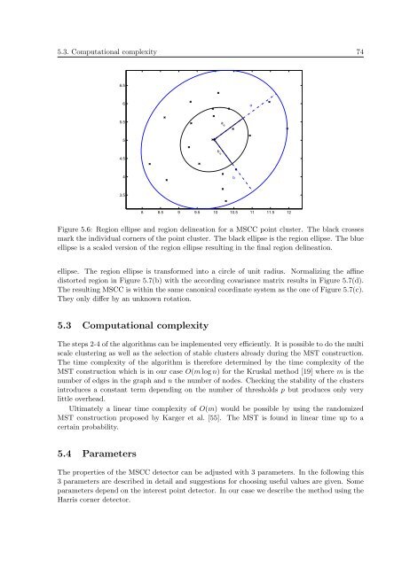
Figure 5.6: Region ellipse and region delineation for a MSCC point cluster. The black crosses
mark the individual corners of the point cluster. The black ellipse is the region ellipse. The blue
ellipse is a scaled version of the region ellipse resulting in the final region delineation.
ellipse. The region ellipse is transformed into a circle of unit radius. Normalizing the affine
distorted region in Figure 5.7(b) with the according covariance matrix results in Figure 5.7(d).
The resulting MSCC is within the same canonical coordinate system as the one of Figure 5.7(c).
They only differ by an unknown rotation.
5.3 Computational complexity
The steps 2-4 of the algorithms can be implemented very efficiently. It is possible to do the multi
scale clustering as well as the selection of stable clusters already during the MST construction.
The time complexity of the algorithm is therefore determined by the time complexity of the
MST construction which is in our case O(m log n) for the Kruskal method [19] where m is the
number of edges in the graph and n the number of nodes. Checking the stability of the clusters
introduces a constant term depending on the number of thresholds p but produces only very
little overhead.
Ultimately a linear time complexity of O(m) would be possible by using the randomized
MST construction proposed by Karger et al. [55]. The MST is found in linear time up to a
certain probability.
5.4 Parameters
The properties of the MSCC detector can be adjusted with 3 parameters. In the following this
3 parameters are described in detail and suggestions for choosing useful values are given. Some
parameters depend on the interest point detector. In our case we describe the method using the
Harris corner detector.