

Student Seminar: Classical and Quantum Integrable Systems
Student Seminar: Classical and Quantum Integrable Systems
Student Seminar: Classical and Quantum Integrable Systems

You also want an ePaper? Increase the reach of your titles
YUMPU automatically turns print PDFs into web optimized ePapers that Google loves.
Preprint typeset in JHEP style - HYPER VERSION<br />
<strong>Student</strong> <strong>Seminar</strong>:<br />
<strong>Classical</strong> <strong>and</strong> <strong>Quantum</strong> <strong>Integrable</strong> <strong>Systems</strong><br />
Gleb Arutyunov a<br />
a Institute for Theoretical Physics <strong>and</strong> Spinoza Institute, Utrecht University<br />
3508 TD Utrecht, The Netherl<strong>and</strong>s<br />
Abstract: The students will be guided through the world of classical <strong>and</strong> quantum<br />
integrable systems. Starting from the famous Liouville theorem <strong>and</strong> finitedimensional<br />
integrable models, the basic aspects of integrability will be studied including<br />
elements of the modern classical <strong>and</strong> quantum soliton theory, the Riemann-<br />
Hilbert factorization problem <strong>and</strong> the Bethe ansatz.<br />
Delivered at Utrecht University, 20 September 2006- 24 January 2007
Contents<br />
1. Liouville Theorem 2<br />
1.1 Dynamical systems of classical mechanics 2<br />
1.2 Harmonic oscillator 5<br />
1.3 The Liouville theorem 7<br />
1.4 Action-angle variables 9<br />
2. Examples of integrable models solved by Liouville theorem 11<br />
2.1 Some general remarks 11<br />
2.2 The Kepler two-body problem 12<br />
2.2.1 Central fields in which all bounded orbits are closed. 15<br />
2.2.2 The Kepler laws 17<br />
2.3 Rigid body 20<br />
2.3.1 Moving coordinate system 20<br />
2.3.2 Rigid bodies 21<br />
2.3.3 Euler’s top 23<br />
2.3.4 On the Jacobi elliptic functions 27<br />
2.3.5 Mathematical pendulum 29<br />
2.4 <strong>Systems</strong> with closed trajectories 31<br />
3. Lax pairs <strong>and</strong> classical r-matrix 32<br />
3.1 Lax representation 32<br />
3.2 Lax representation with a spectral parameter 34<br />
3.3 The Zakharov-Shabat construction 36<br />
4. Two-dimensional integrable PDEs 41<br />
4.1 General remarks 42<br />
4.2 Soliton solutions 43<br />
4.2.1 Korteweg-de-Vries cnoidal wave <strong>and</strong> soliton 43<br />
4.2.2 Sine-Gordon cnoidal wave <strong>and</strong> soliton 45<br />
4.3 Zero-curvature representation 47<br />
4.4 Local integrals of motion 49<br />
5. <strong>Quantum</strong> <strong>Integrable</strong> <strong>Systems</strong> 55<br />
5.1 Coordinate Bethe Ansatz (CBA) 56<br />
5.2 Algebraic Bethe Ansatz 68<br />
5.3 Nested Bethe Ansatz (to be written) 79<br />
6. Introduction to Lie groups <strong>and</strong> Lie algebras 80<br />
– 1 –
7. Homework exercises 95<br />
7.1 <strong>Seminar</strong> 1 95<br />
7.2 <strong>Seminar</strong> 2 96<br />
7.3 <strong>Seminar</strong> 3 97<br />
7.4 <strong>Seminar</strong> 4 98<br />
7.5 <strong>Seminar</strong> 5 100<br />
7.6 <strong>Seminar</strong> 6 102<br />
7.7 <strong>Seminar</strong> 7 105<br />
7.8 <strong>Seminar</strong> 8 107<br />
1. Liouville Theorem<br />
1.1 Dynamical systems of classical mechanics<br />
To motivate the basic notions of the theory of Hamiltonian dynamical systems consider<br />
a simple example.<br />
Let a point particle with mass m move in a potential U(q), where q = (q 1 , . . . q n )<br />
is a vector of n-dimensional space. The motion of the particle is described by the<br />
Newton equations<br />
m¨q i = − ∂U<br />
∂q i<br />
Introduce the momentum p = (p 1 , . . . , p n ), where p i = m ˙q i <strong>and</strong> introduce the energy<br />
which is also know as the Hamiltonian of the system<br />
H = 1<br />
2m p2 + U(q) .<br />
Energy is a conserved quantity, i.e. it does not depend on time,<br />
dH<br />
dt = 1 m p iṗ i + ˙q i ∂U<br />
∂q i = 1 m m2 ˙q i¨q i + ˙q i ∂U<br />
∂q i = 0<br />
due to the Newton equations of motion.<br />
Having the Hamiltonian the Newton equations can be rewritten in the form<br />
˙q j = ∂H<br />
∂p j<br />
,<br />
ṗ j = − ∂H<br />
∂q j .<br />
These are the fundamental Hamiltonian equations of motion. Their importance lies<br />
in the fact that they are valid for arbitrary dependence of H ≡ H(p, q) on the<br />
dynamical variables p <strong>and</strong> q.<br />
– 2 –
The last two equations can be rewritten in terms of the single equation. Introduce<br />
two 2n-dimensional vectors<br />
( ) p<br />
x = , ∇H =<br />
q<br />
(<br />
∂H<br />
)<br />
∂p j<br />
∂H<br />
∂q j<br />
<strong>and</strong> 2n × 2n matrix J:<br />
J =<br />
( ) 0 −I<br />
I 0<br />
Then the Hamiltonian equations can be written in the form<br />
ẋ = J · ∇H , or J · ẋ = −∇H .<br />
In this form the Hamiltonian equations were written for the first time by Lagrange<br />
in 1808.<br />
Vector x = (x 1 , . . . , x 2n ) defines a state of a system in classical mechanics. The<br />
set of all these vectors form a phase space M = {x} of the system which in the present<br />
case is just the 2n-dimensional Euclidean space with the metric (x, y) = ∑ 2n<br />
i=1 xi y i .<br />
The matrix J serves to define the so-called Poisson brackets on the space F(M)<br />
of differentiable functions on M:<br />
{F, G}(x) = (∇F, J∇G) = J ij ∂ i F ∂ j G =<br />
n∑<br />
j=1<br />
( ∂F<br />
∂p j<br />
∂G<br />
∂q j − ∂F<br />
∂q j ∂G<br />
∂p j<br />
)<br />
.<br />
Problem. Check that the Poisson bracket satisfies the following conditions<br />
{F, G} = −{G, F } ,<br />
{F, {G, H}} + {G, {H, F }} + {H, {F, G}} = 0<br />
for arbitrary functions F, G, H.<br />
Thus, the Poisson bracket introduces on F(M) the structure of an infinitedimensional<br />
Lie algebra. The bracket also satisfies the Leibnitz rule<br />
{F, GH} = {F, G}H + G{F, H}<br />
<strong>and</strong>, therefore, it is completely determined by its values on the basis elements x i :<br />
{x j , x k } = J jk<br />
– 3 –
which can be written as follows<br />
{q i , q j } = 0 , {p i , p j } = 0 , {p i , q j } = δj i .<br />
The Hamiltonian equations can be now rephrased in the form<br />
ẋ j = {H, x j } ⇔ ẋ = {H, x} = X H .<br />
A Hamiltonian system is characterized by a triple (M, {, }, H): a phase space<br />
M, a Poisson structure {, } <strong>and</strong> by a Hamiltonian function H. The vector field X H<br />
is called the Hamiltonian vector field corresponding to the Hamiltonian H. For any<br />
function F = F (p, q) on phase space, the evolution equations take the form<br />
dF<br />
dt = {H, F }<br />
Again we conclude from here that the Hamiltonian H is a time-conserved quantity<br />
dH<br />
dt<br />
= {H, H} = 0 .<br />
Thus, the motion of the system takes place on the subvariety of phase space defined<br />
by H = E constant.<br />
In the case under consideration the matrix J is non-degenerate so that there<br />
exist the inverse<br />
J −1 = −J<br />
which defines a skew-symmetric bilinear form ω on phase space<br />
ω(x, y) = (x, J −1 y) .<br />
In the coordinates we consider it can be written in the form<br />
ω = ∑ j<br />
dp j ∧ dq j .<br />
This form is closed, i.e. dω = 0.<br />
A non-degenerate closed two-form is called symplectic <strong>and</strong> a manifold endowed<br />
with such a form is called a symplectic manifold. Thus, the phase space we consider<br />
is the symplectic manifold.<br />
Imagine we make a change of variables y j = f j (x k ). Then<br />
ẏ j = ∂yj<br />
}{{} ∂x k<br />
A j k<br />
ẋ k = A j k J km ∇ x mH = A j km ∂yp<br />
kJ ∂x m ∇y pH<br />
– 4 –
or in the matrix form<br />
ẏ = AJA t · ∇ y H .<br />
The new equations for y are Hamiltonian if <strong>and</strong> only if<br />
AJA t = J<br />
<strong>and</strong> the new Hamiltonian is ˜H(y) = H(x(y)).<br />
Transformation of the phase space which satisfies the condition<br />
AJA t = J<br />
is called canonical. In case A does not depend on x the set of all such matrices form<br />
a Lie group known as the real symplectic group Sp(2n, R) . The term “symplectic<br />
group” was introduced by Herman Weyl. The geometry of the phase space which<br />
is invariant under the action of the symplectic group is called symplectic geometry.<br />
Symplectic (or canonical) transformations do not change the symplectic form ω:<br />
ω(Ax, Ay) = −(Ax, JAy) = −(x, A t JAy) = −(x, Jy) = ω(x, y) .<br />
In the case we considered the phase space was Euclidean: M = R 2n . This is not<br />
always so. The generic situation is that the phase space is a manifold. Consideration<br />
of systems with general phase spaces is very important for underst<strong>and</strong>ing the<br />
structure of the Hamiltonian dynamics.<br />
1.2 Harmonic oscillator<br />
Historically it is proved to be difficult to find a dynamical system such that the<br />
Hamiltonian equations could be solved exactly. However, there is a general framework<br />
where the explicit solutions of the Hamiltonian equations can be constructed. This<br />
construction involves<br />
• solving a finite number of algebraic equations<br />
• computing finite number of integrals.<br />
If this is the way to find a solution then one says it is obtained by quadratures.<br />
The dynamical systems which can be solved by quadratures constitute a special<br />
class which is known as the Liouville integrable systems because they satisfy the<br />
requirements of the famous Liouville theorem. The Liouville theorem essentially<br />
states that if for a dynamical system defined on the phase space of dimension 2n one<br />
finds n independent functions F i which Poisson commute with each other: {F i , F j } =<br />
0 then this system van be solved by quadratures.<br />
– 5 –
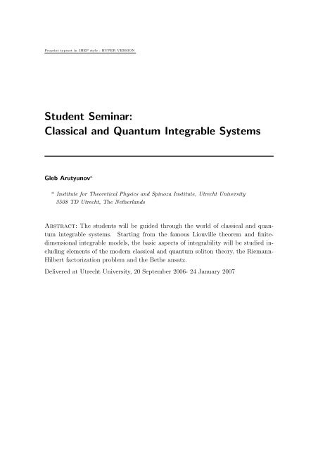
To get more insight on the Liouville theorem let us consider the simplest example<br />
– harmonic oscillator. The phase space has dimension 2 <strong>and</strong> the Hamiltonian is<br />
H = 1 2 (p2 + ω 2 q 2 ) ,<br />
while the Poisson bracket is {p, q} = 1. Energy is conserved, therefore, the phase<br />
space is fibred into ellipses H = E.<br />
p<br />
stationary point<br />
H=E=const −−energy levels<br />
q<br />
HARMONIC OSCILLATOR −− PROTOTYPE OF LIOUVILLE INTEBRABLE SYSTEMS<br />
Problem.<br />
system<br />
Rewrite the Poisson bracket {p, q} = 1 <strong>and</strong> the Hamiltonian in the new coordinate<br />
p = ρ cos(θ) , q = ρ ω sin(θ) .<br />
The answer is<br />
The hamiltonian is<br />
{ρ, θ} = ω ρ .<br />
H = 1 2 ρ2 → ρ = √ 2H .<br />
We see that ρ is an integral of motion. Equation for θ:<br />
˙θ = {H, θ} = ρ{ρ, θ} = ω ⇒ θ(t) = ωt + θ 0 .<br />
This means that the flow takes place on the ellipsis with the fixed value of ρ.<br />
Generalization to n harmonic oscillators is easy:<br />
H =<br />
n∑<br />
i=1<br />
1<br />
2 (p2 i + ω 2 i q 2 i ) .<br />
– 6 –
Commuting integrals<br />
F i = 1 2 (p2 i + ω 2 i q 2 i ) .<br />
Define the common level manifold<br />
M f = {x ∈ M : F i = f i , i = 1, . . . , M}<br />
This manifold is isomorphic to n-dimensional real torus which is a cartesian product<br />
of n topological circles. These tori foliate the phase space <strong>and</strong> can be parametrized<br />
with n angle variables θ i which evolve linearly in time with frequencies ω i . This<br />
motion is conditionally periodic: if all the periods T i = 2π<br />
ω i<br />
are rationally dependent:<br />
T i<br />
T j<br />
= rational number<br />
the motion is periodic, otherwise the flow is dense on the torus.<br />
1.3 The Liouville theorem<br />
The system is Liouville integrable if it possesses n independent conserved quantities<br />
F i , i = 1, . . . , n, {H, F i } which are in involution<br />
{F i , F j } = 0 .<br />
The Liouville theorem. Suppose that we are given n functions in involution on a<br />
symplectic 2n-dimensional manifold<br />
Consider a level set of the functions F i :<br />
F 1 , . . . , F n , {F i , F j } = 0 .<br />
M f = {x ∈ M : F i = f i , i = 1, . . . , n}<br />
Assume that the n functions F i are independent on M f . In other words, the n-forms<br />
dF i are linearly independent at each point of M f . Then<br />
1. M f is a smooth manifold, invariant under the flow with H = H(F i ).<br />
2. If the manifold M is compact <strong>and</strong> connected then it is diffeomorphic to the<br />
n-dimensional torus<br />
T n = {(ψ 1 , . . . , ψ n ) mod 2π}<br />
3. The phase flow with the Hamiltonian function H determines a conditionally<br />
periodic motion on M f , i.e. in angular variables<br />
dψ i<br />
dt = ω i , ω i = ω i (F j ) .<br />
– 7 –
4. The equations of motion with Hamiltonian H can be integrated by quadratures.<br />
Let us outline the proof. Consider the level set of the integrals<br />
M f = {x ∈ M : F i = f i , i = 1, . . . , M} .<br />
By assumptions, the n one-forms dF i are linearly independent at each point of M f ;<br />
by the implicit function theorem, M f is an n-dimensional submanifold on the 2ndimensional<br />
phase space M. Moreover, the n linearly-independent vector fields<br />
ξ Fi = {F i , . . .}<br />
are tangent to M f <strong>and</strong> commute with each other.<br />
Let α = ∑ i p idq i be the canonical 1-form <strong>and</strong> ω = dα = ∑ i dp i ∧ dq i is the<br />
symplectic form on the phase space M. Consider a canonical transformation<br />
i.e.<br />
(p i , q i ) → (F i , ψ i )<br />
ω = ∑ i<br />
dp i ∧ dq i = ∑ i<br />
dF i ∧ dψ i<br />
such that F i are treated as the new momenta. If we found this transformation then<br />
equations of motion read as<br />
˙ F j = {H, F j } = 0 ,<br />
˙ψ j = {H, ψ j } = ∂H<br />
∂F j<br />
= ω j .<br />
Thus, ω i are constant in time. In these coordinates equations of motion are solved<br />
trivially<br />
F j (t) = F j (0) , ψ j (t) = ψ j (0) + tω j .<br />
Thus, we see that the basic problem is to construct a canonical transformation<br />
(p i , q i ) → (F i , ψ i ). This is usually done with the help of the so-called generating<br />
function S. Consider M f : F i (p, q) = f i <strong>and</strong> solve for p i : p i = p i (f, q). Consider the<br />
function<br />
We see that<br />
<strong>and</strong> we further define<br />
S(f, q) =<br />
∫ m<br />
m 0<br />
α =<br />
∫ q<br />
p j = ∂S<br />
∂q j<br />
ψ j = ∂S<br />
∂f j<br />
q 0<br />
∑<br />
i<br />
p i (f, ˜q)d˜q i<br />
– 8 –
Thus, we have<br />
Since d 2 S = 0 we get<br />
i.e. the transformation is canonical.<br />
dS = ∂S<br />
∂q j<br />
dq j + ∂S<br />
∂f j<br />
df j = p j dq j + ψ j df j<br />
∑<br />
dp j ∧ dq j = ∑<br />
j<br />
j<br />
df j ∧ dψ j ,<br />
The next point is to show that S exists, i.e. it does not depend on the path. If<br />
we have a closed path from m 0 to m <strong>and</strong> from m to m 0 <strong>and</strong> assume that M f does<br />
not have non-trivial cycles then by the Stokes theorem we get<br />
∫ m0<br />
∫ ∫<br />
∆S = α = dα = ω = 0<br />
m 0<br />
because the form ω vanishes on M f :<br />
ω(ξ Fi , ξ Fj ) = {F i , F j } = 0 .<br />
In case the manifold M f has non-trivial cycles the situation changes <strong>and</strong> one gets<br />
the change of S given by integral of α over a cycle<br />
∫<br />
∆ cycle S = α<br />
which is a function of F i only! This tells us that in this case the variables ψ j are<br />
multi-valued.<br />
cycle<br />
Mention Darboux<br />
1.4 Action-angle variables<br />
As follows from the Liouville theorem under suitable assumptions of compactness<br />
<strong>and</strong> connectedness motion of a dynamical system in the 2n-dimensional phase space<br />
happens on a n-dimensional torus T n being a common level of n commuting integrals<br />
of motion. The torus has n fundamental cycles C j which allow to introduce the<br />
“normalized” action variables<br />
I j = 1<br />
2π<br />
∮<br />
C j<br />
p i (q, f)dq i ≡ 1<br />
2π<br />
∮<br />
C j<br />
α ,<br />
where f i define the common level T n of the commuting integrals F i . The variables<br />
I j are functions of f i only <strong>and</strong> therefore they are constants of motion. The angle<br />
variables are introduced as independent angle coordinates on the cycles<br />
1<br />
2π<br />
∮<br />
C j<br />
dθ i = δ ij .<br />
– 9 –
Let us show that the variables (I i , θ i ) are canonically conjugate. For that we need<br />
to construct a canonical transformation (p i , q i ) → (I i , θ i ). Consider a generating<br />
function depending on I i <strong>and</strong> q i :<br />
We see that<br />
Let us introduce<br />
S(I, q) =<br />
∫ m<br />
m 0<br />
α =<br />
∫ q<br />
q 0<br />
p i (q ′ , I)dq ′ i .<br />
p j = ∂S<br />
∂q j<br />
=⇒ p = p(q, I).<br />
θ j = ∂S<br />
∂I j<br />
=⇒ θ = θ(q, I).<br />
<strong>and</strong> show that θ j are indeed coincide with the properly normalized angle variables.<br />
We have<br />
∮<br />
1<br />
dθ i = 1 ∮<br />
d ∂S = ∂ ( ∮ 1<br />
)<br />
dS = ∂ ( ∮ 1 ∂S<br />
dq k +<br />
∂S dI k<br />
2π C j<br />
2π C j<br />
∂I i ∂I i 2π C j<br />
∂I i 2π C j<br />
∂q k ∂I<br />
} {{ k<br />
}<br />
Furthermore,<br />
= ∂ ( ∮ 1<br />
)<br />
α = δ ij .<br />
∂I i 2π C j<br />
=0 on C j<br />
)<br />
( ∂S<br />
) (<br />
dI i ∧ dθ i = −d(θ i dI i ) = −d dI i = −d dS − ∂S )<br />
dq i = d(p i dq i ) = dp i ∧ dq i .<br />
∂I i ∂q i<br />
Problem. Find action-angle variables for the harmonic oscillator.<br />
We have<br />
E = 1 2 (p2 + ω 2 q 2 ) =⇒ p(E, q) = ± √ 2E − ω 2 q 2 .<br />
<strong>and</strong>, therefore,<br />
I = 1 ∮<br />
dq √ 2E − ω<br />
2π<br />
2 q 2 = 2<br />
E<br />
2π<br />
∫ √ 2E<br />
ω<br />
− √ 2E<br />
ω<br />
The generating function of the canonical transformation reads<br />
while for the angle variables we obtain<br />
S(I, q) = ω<br />
∫ q<br />
dx √ 2I − x 2 ,<br />
dq √ 2E − ω 2 q 2 = E ω .<br />
θ = ∂S<br />
∂I = ω ∫ q<br />
dx<br />
√<br />
2I − x<br />
2 = ω arctan<br />
q<br />
√<br />
2I − q<br />
2<br />
=⇒ q = √ 2I sin θ ω .<br />
Finally, we explicitly check that the transformation to the action-angle variables is canonical<br />
(<br />
dI<br />
dp ∧ dq = ω √ −<br />
2I − q<br />
2<br />
qdq<br />
)<br />
√ ∧ dq =<br />
2I − q<br />
2<br />
ω<br />
√<br />
2I − q<br />
2 dI ∧ d(√ 2I sin θ ω<br />
)<br />
= dI ∧ dθ .<br />
– 10 –
2. Examples of integrable models solved by Liouville theorem<br />
2.1 Some general remarks<br />
Problem. Consider motion in the potential<br />
V (q) =<br />
Solve eoms <strong>and</strong> find a period of oscillations. One has<br />
t − t 0 =<br />
∫ q<br />
q 0<br />
dq<br />
√<br />
= −<br />
2(E − g2<br />
sin 2 q )<br />
∫ q<br />
q 0<br />
g2<br />
sin 2 q , E > g2 .<br />
d cos q<br />
√ √<br />
2E<br />
(E−g 2 )<br />
E<br />
− cos 2 q<br />
∫ arccos q<br />
= −<br />
arccos q 0<br />
Thus, motion happens on the interval q 0 < q < π − q 0 <strong>and</strong> taking q 0 = arcsin<br />
We see from here that<br />
Period is<br />
cos √ } {{<br />
2E<br />
}<br />
ω<br />
It does not depend on g 2 !!!<br />
t = − 1 √<br />
2E<br />
(<br />
arcsin<br />
x<br />
√<br />
E−g 2<br />
E<br />
( π<br />
t = cos<br />
2 − arcsin x<br />
)<br />
√ =<br />
1 − g2<br />
E<br />
T = 2π ω =<br />
)<br />
2π √<br />
2E<br />
.<br />
| x=cos q<br />
q<br />
E−g<br />
x=<br />
2<br />
E<br />
x<br />
√<br />
1 − g2<br />
E<br />
dx<br />
√ √ .<br />
2E<br />
(E−g 2 )<br />
E<br />
− x 2<br />
√<br />
g 2<br />
E<br />
= √<br />
1<br />
cos q .<br />
1 − g2<br />
E<br />
one gets<br />
Problem. Consider a one-dimensional harmonic oscillator with the frequency ω <strong>and</strong> compute the<br />
area surrounded by the phase curve corresponding to the energy E. Show that the period of motion<br />
along this phase curve is given by T = dS<br />
dE .<br />
A curve is an ellipsis<br />
( x<br />
a<br />
) 2<br />
+<br />
( y<br />
b<br />
) 2<br />
= 1<br />
with the area<br />
S = 2b<br />
∫ a<br />
−a<br />
dx √ ∫ π √<br />
1 − x 2 /a 2 2<br />
= 2ba dφ cos φ 1 − sin 2 φ = 2ab<br />
− π 2<br />
∫ π<br />
2<br />
− π 2<br />
dφ cos 2 φ = πab .<br />
We have to identify a = ρ, b = ρ ω<br />
so that<br />
S = πab = π ρ2<br />
ω = 2π ω E .<br />
From here we see that<br />
dS<br />
dE = 2π ω = T ,<br />
where T is a period of motion. The last expression has the same form as the first law of thermodynamics<br />
dE = 1 T<br />
dS provided that 1/T is the temperature (the period ≡ the inverse temperature).<br />
Problem. Let E 0 be the value of the potential at a minimum point ξ. Find the period T 0 =<br />
lim E→E0 T (E) of small oscillations in a neighborhood of the point ξ.<br />
– 11 –
We have<br />
H = p2<br />
2<br />
p2<br />
+ V (x) =<br />
2 + V } {{ (ξ) + V ′ (ξ)(x − ξ) + 1 } } {{ } 2 V ′′ (ξ)(x − ξ) 2 + · · ·<br />
const =0<br />
Effectively we have motion described by the harmonic oscillator with the Hamiltonian<br />
H eff = p2<br />
2 + 1 2 V ′′ (ξ)q 2<br />
whose frequency is ω = √ V ′′ (ξ). Therefore the period of small oscillations is<br />
T 0 =<br />
2π<br />
√<br />
V<br />
′′<br />
(ξ) .<br />
2.2 The Kepler two-body problem<br />
Here we consider one of the historically first examples of integrable systems solved<br />
by the Liouville theorem: The Kepler two-body problem of planetary motion.<br />
In the center of mass frame eoms are<br />
d 2 x i<br />
dt 2<br />
(r)<br />
= −∂V , r =<br />
∂x i<br />
√<br />
x 2 1 + x 2 2 + x 2 3<br />
In the original Kepler problem V (r) = − k , k > 0. The Hamiltonian<br />
r<br />
H = 1 2<br />
3∑<br />
p 2 i + V (r)<br />
i=1<br />
<strong>and</strong> the bracket {p i , x j } = δ ij .<br />
Problem . Show that the angular momentum<br />
⃗J = (J 1 , J 2 , J 3 ) ,<br />
J ij = x i p j − x j p i = ɛ ijk J k<br />
is conserved.<br />
J˙<br />
ij = ẋ i p j − x i ṗ j − (i ↔ j) = p i p j + ∂V<br />
∂r x ∂r<br />
i − (i ↔ j) = ∂V<br />
∂x j ∂r<br />
Note that this is a consequence of the central symmetry.<br />
(<br />
x i<br />
∂r<br />
∂x j<br />
− x j<br />
∂r<br />
∂x i<br />
)<br />
= 0<br />
Problem. Compute the Poisson brackets<br />
Show that there are three commuting quantities<br />
{J i , J j } = −ɛ ijk J k<br />
H, J 3 , J 2 = J 2 1 + J 2 2 + J 2 3<br />
Rewrite the canonical one form in the polar coordinates<br />
x 1 = r sin θ cos φ, x 2 = r sin θ sin φ, x 3 = r cos θ<br />
– 12 –
We find<br />
α = ∑ i<br />
p i dx i = p r dr + p θ dθ + p φ dφ ,<br />
where the original momenta are expressed as<br />
p 1 = 1 (<br />
sin φ<br />
)<br />
rp r cos φ sin θ + p θ cos θ cos φ − p φ ,<br />
r<br />
sin θ<br />
p 2 = 1 (<br />
cos φ<br />
)<br />
rp r sin φ sin θ + p θ cos θ sin φ + p φ ,<br />
r<br />
sin θ<br />
p 3 = p r cos θ − 1 r p θ sin θ .<br />
Conserved quantities<br />
(<br />
p 2 r + 1 r 2 p2 θ +<br />
H = 1 2<br />
J 2 = p 2 θ + 1<br />
sin 2 θ p2 φ<br />
J 3 = p φ<br />
1<br />
)<br />
r 2 sin 2 θ p2 φ + V (r)<br />
To better underst<strong>and</strong> the physics we note that the motion happens in the plane<br />
orthogonal to the vector J. ⃗ Without loss of generality we can rotate our coordinate<br />
system such that in a new system J ⃗ has only the third component: J ⃗ = (0, 0, J3 ).<br />
This simply accounts in putting in our previous formulae θ = π . Then we note that<br />
2<br />
p 2 φ<br />
˙φ = {H, φ} = {<br />
2r 2 sin 2 θ , φ} =<br />
that for θ = π 2 expresses the integral of motion p φ as<br />
p φ = r 2 ˙φ.<br />
p φ<br />
r 2 sin 2 θ<br />
This is the conservation law of angular momentum discovered by Kepler through<br />
observations of the motion of Mars. The quantity p φ = J has a simple geometric<br />
meaning. Kepler introduced the sectorial velocity C:<br />
C = dS<br />
dt ,<br />
where ∆S is an area of the infinitezimal sector swept by the radius-vector ⃗r for time<br />
∆t:<br />
∆S = 1 2 r · r ˙φ∆t + O(∆t 2 ) ≈ 1 2 r2 ˙φ∆t .<br />
This is the (second) law discovered by Kepler: in equal times the radius vector sweeps<br />
out equal areas, so the sectorial velocity is constant. This is one of the formulations<br />
of the conservation law of angular momentum. 1<br />
1 Some satellites have very elongated orbits. According to Kepler’s law such a satellite spends<br />
most of its time in the distant part of the orbit where the velocity ˙φ is small.<br />
– 13 –
We can now see how the solution can be found by using the general approach<br />
based on the Liouville theorem. The expressions for the momenta on the surface of<br />
constant energy <strong>and</strong> J = J 3 are<br />
√<br />
p r = 2(H − V ) − J 2<br />
r , p 2 φ = J 3 = J .<br />
We can thus construct the generating function of the canonical transformation from<br />
from the Liouville theorem<br />
∫ r<br />
S =<br />
√2(H − V ) − J ∫ 2 φ<br />
r + Jdφ<br />
2<br />
<strong>and</strong> the associated angle variables<br />
We have eoms<br />
Integrating the first one we obtain<br />
ψ H = ∂S<br />
∂H ,<br />
ψ J = ∂S<br />
∂J<br />
˙ψ H = 1 , ˙ψ J = 0 .<br />
<strong>and</strong>, therefore,<br />
The equation for ψ J gives<br />
ψ J = −<br />
t − t 0 =<br />
∫ r<br />
ψ H = t − t 0<br />
∫ r<br />
dr<br />
√<br />
.<br />
2(H − V ) − J2<br />
r 2<br />
Jdr<br />
√<br />
+ φ = 0 ,<br />
r 2 2(H − V ) − J2<br />
r 2<br />
so that<br />
φ =<br />
∫ r<br />
Jdr<br />
√<br />
r 2 2 ( ) .<br />
E − V (r) − J 2<br />
2r 2<br />
Generically, equation which defines the values of r at which ṙ = 0:<br />
E − V (r) − J 2<br />
2r 2 = 0<br />
has two solutions: r min <strong>and</strong> r max , they are called pericentum <strong>and</strong> apocentrum respectively<br />
2 . When ṙ = 0, ˙φ ≠ 0. The r oscillates monotonically between rmin <strong>and</strong><br />
2 If the earth is the center then r min <strong>and</strong> r max are called perigee <strong>and</strong> apogee, if the sun – perihelion<br />
<strong>and</strong> apohelion, if the moon – perilune <strong>and</strong> apolune.<br />
– 14 –
max while φ changes monotonically. The angle between neighboring apocenter <strong>and</strong><br />
pericenter is given by<br />
∆φ =<br />
∫ rmax<br />
r min<br />
Jdr<br />
√<br />
r 2 2 ( ) .<br />
E − V (r) − J2<br />
2r 2<br />
Generic orbit is not closed! It is closed only if ∆φ = 2π m , m, n ∈ Z, otherwise it is<br />
n<br />
everywhere dense in the annulus. The annulus might degenerate into a circle.<br />
2.2.1 Central fields in which all bounded orbits are closed.<br />
Determination of a central potential for which all bounded orbits are closed is called<br />
the I.L.F. Bertr<strong>and</strong> problem.<br />
There are only two cases for which bounded orbits are closed<br />
V (r) = ar 2 , a ≥ 0 ,<br />
V (r) = − k r , k ≥ 0 .<br />
To show this we have to solve several problems.<br />
Problem. Show that the angle φ between the pericenter <strong>and</strong> apocenter is equal to the half-period<br />
of an oscillation in the one dimensional system with potential energy W (x) = V (J/x) + x2<br />
2 .<br />
Substitution r = J r gives ∆φ =<br />
∫ xmax<br />
x min<br />
dx<br />
√<br />
2(E − W (x))<br />
.<br />
Problem. Find the angle φ for an orbit close to the circle of radius r.<br />
Effectively the angle φ is described by half-period of oscillation<br />
∆φ =<br />
∫ xmax<br />
x min<br />
dx<br />
√<br />
2(E − W (x))<br />
.<br />
We have<br />
∆φ = π ω , ω = √ W ′′ (x) ,<br />
where x = J r . We find W ′ (x) = ∂ x V (J/x) + x = − J x 2 V ′ (J/x) + x ,<br />
We have to take<br />
W ′′ (x) = 2 J x 3 V ′ (J/x) + J 2<br />
x 4 V ′′ (J/x) + 1 .<br />
− J x 2 V ′ (J/x) + x = 0 =⇒ x3<br />
J = V ′ (J/x) =⇒ J<br />
r 3/2 = √ V ′ (r) .<br />
– 15 –
Thus,<br />
<strong>and</strong>, therefore, the half-period is<br />
W ′′ (x) = J )<br />
(3V ′<br />
x 3 (r) + rV ′′ (r) = 3V ′ (r) + rV ′′ (r)<br />
V ′ (r)<br />
√<br />
V<br />
∆φ circ = π<br />
′ (r)<br />
3V ′ (r) + rV ′′ (r) .<br />
Problem. Find the potentials V for which the magnitude of ∆φ circ does not depend on the radius.<br />
We have to require<br />
( 3V ′ (r) + rV ′′ (r)<br />
V ′ (r)<br />
) ′ ( rV ′′ (r)<br />
) ′ (<br />
= =<br />
V ′ r ( log V ′ (r) ) ) ′<br />
′<br />
= 0 ,<br />
(r)<br />
i.e.<br />
log V ′ (r) = const<br />
∫ 1<br />
r<br />
= s log r + m , s, m = const .<br />
Further,<br />
V ′ (r) = const r s , =⇒ V (r) = ar α ,<br />
or V (r) = b log r if s = −1. Finally, the expression<br />
V (r) = ar α we will get<br />
V ′ (r)<br />
3V ′ (r)+rV ′′ (r)<br />
should be positive. If we take<br />
V ′ (r)<br />
3V ′ (r) + rV ′′ (r) = α<br />
3α + α(α − 1) = 1 > 0 =⇒ α > −2 .<br />
2 + α<br />
Finally, we also have<br />
∆φ circ =<br />
π<br />
√ 2 + α<br />
.<br />
Here the logarithmic case correspond to α = 0. Particular cases are α = 2 which gives ∆φ circ = π 2<br />
<strong>and</strong> α = −1 which gives ∆φ circ = π.<br />
Problem. Let V (r) → ∞ as r → ∞. Find<br />
lim ∆φ circ(E, J)<br />
E→∞<br />
Let us make a substitution x = yx max , we get<br />
∫ 1<br />
dy<br />
∆φ circ = √<br />
y min 2(Q(1) − Q(y))<br />
(<br />
where Q(y) = y2<br />
2 + 1 J<br />
x<br />
V 2<br />
max yx max<br />
). As E → ∞ we have x max → ∞ <strong>and</strong> y min → 0 <strong>and</strong> the second<br />
term in Q can be discarded. Thus, we get<br />
∆φ circ =<br />
∫ 1<br />
0<br />
dy<br />
√<br />
1 − y<br />
2 = π 2 .<br />
Problem. Let V (r) = −kr −β , where 0 < β < 2. Find<br />
lim ∆φ circ(E, J)<br />
E→−0<br />
– 16 –
One has<br />
∆φ circ =<br />
∫ xmax<br />
x min<br />
dx<br />
√<br />
2E + 2k x<br />
J β − x 2<br />
β<br />
E→0<br />
→<br />
∫ xmax<br />
x min<br />
dx<br />
√<br />
2k<br />
x<br />
J β − x 2<br />
β<br />
Rescale x = αy with α satisfying the relation 2k<br />
J β α β = α 2 , then we get<br />
∆φ circ =<br />
∫ 1<br />
We note that the result does not depend on J.<br />
0<br />
dy<br />
√<br />
yβ − y = π<br />
2 2 − β .<br />
Now we are ready to find the potentials for which all bounded orbits are closed. If<br />
all bounded orbits are closed, then, in particular, ∆φ circ = 2π m = const. That means<br />
n<br />
that ∆φ circ should not depend on the radius, which is the case for the potentials<br />
V (r) = ar α , α > −2 <strong>and</strong> V (r) = b log r .<br />
In both cases ∆φ circ = √ π<br />
2+α<br />
. If α > 0 then lim E→∞ ∆φ circ (E, J) = π <strong>and</strong> therefore<br />
2<br />
α = 2. If α < 0 then lim E→0 ∆φ circ (E, J) = π . Then we have an equality<br />
2+α<br />
π<br />
= √ π<br />
2+α 2+α<br />
which gives α = −1. In the case α = 0 we find ∆φ circ = √ π 2<br />
which<br />
is not commensurable with 2π. Therefore all bounded orbits are closed only for<br />
V = ar 2 <strong>and</strong> U = − k .<br />
r 2<br />
2.2.2 The Kepler laws<br />
For the original Kepler problem we have<br />
<strong>and</strong><br />
Integrating we get<br />
∫<br />
φ =<br />
V (r) = − k r + J 2<br />
2r 2 .<br />
Jdr<br />
√<br />
r 2 2(E + k − J 2<br />
)<br />
r 2r 2<br />
φ = arccos<br />
J<br />
√ − k r J<br />
.<br />
2E + k2<br />
J 2<br />
An integration constant is chosen to be zero which corresponds to the choice of an<br />
origin of reference for the angle φ at the pericenter. Introduce the notation<br />
√<br />
J 2<br />
k = p , 1 + 2EJ 2<br />
= e ,<br />
k 2<br />
This leads to<br />
r =<br />
p<br />
1 + e cos φ<br />
– 17 –
This is the so-called focal equation of a conic section. When e < 1, i.e. E < 0, the<br />
conic section is an ellipse. The number p is called a parameter of the ellipse <strong>and</strong> e<br />
the essentricity. The motion is bounded for E < 0.<br />
The semi-axis a is determined as<br />
2a =<br />
p<br />
1 − e + p<br />
1 + e = 2p<br />
1 − e . 2<br />
We also have<br />
Thus,<br />
c = a −<br />
p<br />
1 + e = 1 ( p<br />
2 1 − e − p )<br />
= ep<br />
1 + e 1 − e . 2<br />
c<br />
a = e .<br />
b a p<br />
c O<br />
p<br />
p<br />
1−e 1+e<br />
Keplerian ellipse<br />
Obviously, we have three distinguished points<br />
φ = 0 : r = p<br />
1 + e ,<br />
φ = π 2 : r = p ,<br />
We can now formulate the Kepler laws:<br />
φ = π : r = p<br />
1 − e .<br />
1. The first law: Planets describe ellipses with the Sun at one focus.<br />
2. The second law: The sectorial velocity is constant.<br />
3. The third law: The period of revolution around an elliptical orbit depends only<br />
on the size of the major semi-axes. The squares of the revolution periods of<br />
two planets on different elliptical orbits have the same ratio as the cubes of<br />
their major semi-axes.<br />
Let us prove the third law. Let T be a revolutionary period <strong>and</strong> S be the area swept<br />
out by the radius vector over the period. We have<br />
S = πab = πa 2√ √<br />
1 − e 2 = π 1 − e2 = π<br />
(1 − e 2 ) 2 (1 − e 2 ) 3 2<br />
p 2<br />
p 2<br />
= πkJ<br />
( √ 2|E|) 3 ,<br />
– 18 –
while<br />
i.e.<br />
a =<br />
p<br />
1 − e = k<br />
2 2|E| .<br />
On the other h<strong>and</strong>, since the sectorial velocity C is constant we have<br />
∫ T<br />
0<br />
C =<br />
∫ T<br />
0<br />
dt dS<br />
dt = S , =⇒ CT = J 2 T = S ,<br />
T = 2S J =<br />
2πk<br />
( √ 2|E|) = √ 2π a 3 2 .<br />
3 k<br />
It is interesting to note that the total energy depends only on the major semi-axis<br />
a <strong>and</strong> it is the same for the whole set of elliptical orbits from a circle of radius a<br />
to a line segment of length 2a. The value of the second semi-axis do depend on the<br />
angular momentum.<br />
The Runge-Lenz vector <strong>and</strong> the Liouville torus. The phase space of the motion in the<br />
central field is T ∗ R 3 , i.e. it is six-dimensional. There are four conserved integrals:<br />
three components of the angular momentum J i <strong>and</strong> the energy E. This shows that<br />
the motion happens on the two-dimensional manifold. In case of the bounded motion<br />
it is the two-dimensional Liouville torus. Thus, there are two frequencies associated<br />
<strong>and</strong> when they are not rationally commensurable the orbits are not closed but rather<br />
dense on the torus. For the specific Kepler motion (with any sign of k) there is one<br />
more non-trivial conserved quantity appears which is absent for a generic central<br />
potential: The Runge-Lenz vector (for definiteness we assume that k > 0):<br />
⃗R = ⃗v × ⃗ J − k ⃗r r .<br />
Problem. Show that the Runge-Lenz vector is conserved.<br />
Indeed, we have<br />
˙⃗R = ˙⃗v ×<br />
}{{}<br />
J ⃗ −k ⃗v r + k⃗r(⃗v⃗r) r 3<br />
m ⃗r×⃗v<br />
= m ˙⃗v × (⃗r × ⃗v) − k ⃗v r + k⃗r(⃗v⃗r) r 3 .<br />
On the other h<strong>and</strong>,<br />
m ˙⃗v = − ∂U ⃗r<br />
∂r r = −k ⃗r r 3<br />
<strong>and</strong>, therefore,<br />
˙⃗R = −k 1 r 3 ⃗r × (⃗r × ⃗v) − k⃗v r + k⃗r(⃗v⃗r) r 3<br />
Further one has to use the formula<br />
⃗r × (⃗r × ⃗v) = (⃗v⃗r)⃗r − r 2 ⃗v<br />
– 19 –
to show that ˙⃗ R = 0. The last formula can be proved by noting that the vector<br />
⃗r × (⃗r × ⃗v) = α⃗r + β⃗v<br />
is orthogonal to ⃗r. Thus, multiplying both sides by ⃗r we get<br />
0 = αr 2 + β(⃗v⃗r) .<br />
On the other h<strong>and</strong>, multiplying both sides by ⃗v we get<br />
(⃗v, ⃗r × (⃗r × ⃗v)) = α(⃗v⃗r) + βv 2<br />
which gives<br />
(⃗v, ⃗r × (⃗r × ⃗v)) = −(⃗r × ⃗v, ⃗r × ⃗v = −r 2 v 2 sin φ = −r 2 v 2 (1 − cos 2 φ)<br />
= −r 2 v 2 + (⃗v⃗r) 2 = α(⃗v⃗r) + βv 2 .<br />
These two equations allows one to find<br />
α = (⃗v⃗r) , β = −r 2 .<br />
2.3 Rigid body<br />
2.3.1 Moving coordinate system<br />
Let K <strong>and</strong> k will be two oriented Euclidean spaces. A motion of K relative to k is<br />
a mapping smoothly depending on t:<br />
D t : K → k ,<br />
which preserves the metric <strong>and</strong> orientation. Every motion can be uniquely written<br />
as the composition of a rotation (D t which maps the origin of K into the origin<br />
of k, i.e. D t is linear mapping) <strong>and</strong> a translation C t : k → k. Let call K <strong>and</strong> k<br />
moving <strong>and</strong> stationary coordinate systems respectively. Let q(t) <strong>and</strong> Q(t) will be the<br />
radius-vector of a point in a stationary <strong>and</strong> moving coordinate systems respectively.<br />
Then<br />
q(t) = D t Q(t) = B t Q(t) + r(t) .<br />
} {{ } }{{}<br />
rotation translation<br />
Differentiating we get an addition formula for velocities<br />
˙q =<br />
ḂQ +B<br />
}{{}<br />
˙Q + ṙ .<br />
transferred rotation<br />
Suppose a point does not move w.r.t. to the moving frame, i.e.<br />
r = ṙ = 0. Then<br />
˙q = ḂQ = ḂB−1 q = Aq ,<br />
˙Q = 0 <strong>and</strong> also that<br />
– 20 –
where A : k → k is a linear operator on k. Since B is a rotation, it is an orthogonal<br />
transformation: BB t = 1. Differentiating w.r.t to t we get<br />
ḂB t + BḂt = 0 =⇒ ḂB −1 + (ḂB−1 ) t = 0 ,<br />
i.e. A is skew-symmetric. On the other h<strong>and</strong>, every skew-symmetric operator from<br />
R 3 to R 3 is the operator of vector multiplication by a fixed vector ω:<br />
˙q = ω × q .<br />
Generically ω depends on t. Thus, in the case of purely rotational motion with ˙Q ≠ 0<br />
we will have<br />
˙q = ω × q + B ˙Q = ω × q<br />
} {{ }<br />
transferred velocity<br />
+ }{{} v ′<br />
relative velocity<br />
.<br />
2.3.2 Rigid bodies<br />
A rigid body is a system of point masses, constrained by holonomic relations expressed<br />
by the fact that the distance between points is constant<br />
|x i − x j | = r ij = const .<br />
If a rigid body moves freely then its center of mass moves uniformly <strong>and</strong> linearly.<br />
A rigid body rotates about its center of mass as if the center of mass were fixed at<br />
a stationary point O. In this way the problem is reduced to a problem with three<br />
degrees of freedom – motion of a rigid body around a fixed point O. The problem of<br />
rotation of rigid body can be studied in more generality without assuming that the<br />
fixed point coincides with the center of mass of a body. Since the Lagrangian function<br />
is invariant under all rotations around O by Noether theorem the components of the<br />
angular momentum M are conserved: Ṁ = 0 . The total energy which is equal to<br />
the kinetic energy is also conserved. Thus, we see that<br />
In the problem of motion of rigid body around a fixed point, in the absence of<br />
outside forces, there are four integrals of motion: three components on M <strong>and</strong> the<br />
energy. Thus, motion happens on a two-dimensional space inside the six-dimensional<br />
phase-space (three rotation angles plus three velocities) :<br />
M f = {M x = f 1 , M y = f 2 , M z = f 3 , E = f 4 > 0 }.<br />
The phase space is a cotangent bundle to SO(3). The manifold M f is invariant: if<br />
the initial conditions of motion give a point on M f then for all time of motion the<br />
point in T SO(3) corresponding to the position <strong>and</strong> velocity of the body remains in<br />
M f . The two-dimensional manifold M f admits a globally defined vector field (this<br />
is the field of velocities of the motion on T SO(3)), it is orientable <strong>and</strong> compact (E<br />
– 21 –
is the bounded kinetic energy). According to the known theorem in topology, a<br />
two-dimensional compact orientable manifold admitting globally defined vector field<br />
is isomorphic to a torus. This is our Liouville torus 3 . According to the Liouville<br />
theorem motion on the torus will be characterized by two frequencies ω 1 <strong>and</strong> ω 2 . If<br />
their ratio is not a rational number then the body never returns to its original state<br />
of motion.<br />
Consider a rigid body rotation around a fixed point O <strong>and</strong> denote by K a coordinate<br />
system rotating with the body around O: in K the body is at rest. Every<br />
vector in K is carried to k by an operator B. By definition of the angular momentum<br />
we have<br />
M = q × m ˙q = m q × (ω × q) .<br />
Denote by J <strong>and</strong> by Ω the angular momentum <strong>and</strong> angular velocity in the moving<br />
frame K. We have<br />
J = m Q × (Ω × Q) .<br />
This defines a linear map A: K → K such that AΩ = J. This operator is symmetric:<br />
(AX, Y ) = (m Q × (X × Q), Y ) = m(Q × X, Q × Y )<br />
because the r.h.s. is symmetric function of X, Y . The operator A is called the inertia<br />
tensor. We see that taking X = Y = Ω we get<br />
E = T = 1 2 (AΩ, Ω) = 1 2 (J, Ω) = m 2 (Q × Ω, Q × Ω) = m 2 ˙Q 2 = m 2 ˙q2 .<br />
being a symmetric operator A is diagonalizable <strong>and</strong> it defines three mutually orthogonal<br />
characteristic directions. In the basis where A is diagonal the inertia operator<br />
<strong>and</strong> the kinetic energy take a very simple form<br />
J i = I i Ω i ,<br />
T = 1 3∑<br />
I i Ω 2 i .<br />
2<br />
The axes of this particular coordinate system are called the principle inertia axes.<br />
Problem. Rewrite expression for energy via the quantities of the stationary frame k.<br />
We have<br />
i=1<br />
E = 1 2 (AΩ, Ω) = 1 2 (J, Ω) = 1 2 (M, ω) = m 2 (q × (q × ω), ω) = m (q × ω, q × ω)<br />
2<br />
= 1 (ω<br />
2 m 2 q 2 − (ωq) 2) = 1 )<br />
2 ω iω j m<br />
(x 2 i δ ij − x i x j .<br />
} {{ }<br />
inertia tensor<br />
3 We cannot use the Liouville theorem to derive this result, because the integrals M i do not<br />
commute with each other <strong>and</strong>, therefore, the Frobenious theorem cannot be applied to deduce that<br />
the level set is a smooth manifold. Nevertheless we can identify the Liouville torus by different<br />
means.<br />
– 22 –
2.3.3 Euler’s top<br />
Consider the motion of a rigid body around a fixed point O. Let J <strong>and</strong> Ω will be<br />
the vector of angular momentum <strong>and</strong> the angular momentum in the body, i.e. in the<br />
moving coordinate system K. We have AΩ = J, where A is the inertia tensor. The<br />
angular momentum M = B t J of the body in space is preserved. Thus, we have<br />
0 = Ṁ = ḂJ + B ˙ J = ḂB−1 M + B ˙ J = ω × M + B ˙ J = B<br />
(<br />
Ω × J + J ˙<br />
)<br />
.<br />
From here we find<br />
dJ<br />
dt = J × Ω = J × A−1 J .<br />
These are the famous Euler equations which describe the motion of the angular momentum<br />
insider the rigid body. If one takes the coordinate adjusted to the principle<br />
axes then one gets the following system of equations<br />
dJ 1<br />
= a 1 J 2 J 3 ,<br />
dt<br />
dJ 2<br />
= a 2 J 3 J 1 ,<br />
dt<br />
dJ 3<br />
= a 3 J 1 J 2 .<br />
dt<br />
Here<br />
a 1 = I 2 − I 3<br />
, a 2 = I 3 − I 1<br />
, a 3 = I 1 − I 2<br />
.<br />
I 2 I 3 I 1 I 3 I 1 I 2<br />
In this way the Euler equations can be viewed as equations for the components of<br />
the angular momentum insider the body.<br />
Consider the energy<br />
H = 1 2 (J, A−1 J) = 1 2<br />
3∑<br />
i=1<br />
J 2 i<br />
I i<br />
.<br />
It is easy to verify explicitly that it is conserved due to eoms:<br />
3∑ J<br />
(<br />
i a1<br />
Ḣ = J i = J 1 J 2 J 3 + a 2<br />
+ a )<br />
3<br />
= 0 .<br />
I i I 1 I 2 I 3<br />
i=1<br />
Verify the conservation of the length of the angular momentum<br />
3∑<br />
(<br />
)<br />
J˙<br />
2 = J i J˙<br />
i = J 1 J 2 J 3 a 1 + a 2 + a 3 = 0 .<br />
i=1<br />
This is of course agrees with the fact that M is conserved <strong>and</strong> that M 2 = J 2 . Thus,<br />
we have proved that the Euler equations have two quadratic integrals: the energy<br />
<strong>and</strong> M 2 = J 2 . Thus, J lies on the intersection of an ellipsoid <strong>and</strong> a sphere:<br />
2E = J 2 1<br />
I 1<br />
+ J 2 2<br />
I 2<br />
+ J 2 3<br />
I 3<br />
, J 2 = J 2 1 + J 2 2 + J 2 3 .<br />
– 23 –
One can study the structure of the curves of intersection by fixing the ellipsoid E > 0<br />
<strong>and</strong> changing the radius J of the sphere.<br />
Note that alternatively the Euler equations can be rewritten as the equations for<br />
the angular velocity Ω:<br />
dΩ 1<br />
dt + I 3 − I 2<br />
Ω 2 Ω 3 = 0 ,<br />
I 1<br />
dΩ 2<br />
dt + I 1 − I 3<br />
Ω 3 Ω 1 = 0 ,<br />
I 2<br />
dΩ 3<br />
dt + I 2 − I 1<br />
Ω 1 Ω 2 = 0.<br />
I 3<br />
We could express Ω 1 <strong>and</strong> Ω 3 from the conservation laws<br />
Ω 2 1<br />
(<br />
)<br />
1 =<br />
(2EI 3 − J 2 ) − I 2 (I 3 − I 2 )Ω 2 2 ,<br />
I 1 (I 3 − I 1 )<br />
Ω 2 1<br />
(<br />
)<br />
3 =<br />
(J 2 − 2EI 1 ) − I 2 (I 2 − I 1 )Ω 2 2 .<br />
I 3 (I 3 − I 1 )<br />
Then plugging this into the Euler equation for Ω 2 we obtain<br />
dΩ 2<br />
dt<br />
=<br />
√<br />
1 ( )(<br />
)<br />
√ (2EI 3 − J 2 ) − I 2 (I 3 − I 2 )Ω 2 2 (J 2 − 2EI 1 ) − I 2 (I 2 − I 1 )Ω 2 2 .<br />
I 2 I1 I 3<br />
We assume that I 3 > I 2 > I 1 <strong>and</strong> further that M 2 > 2EI 2 . Then making the<br />
substitutions<br />
√<br />
√<br />
(I 3 − I 2 )(J<br />
τ = t<br />
− 2EI 1 )<br />
I 2 (I 3 − I 2 )<br />
, s = Ω 2<br />
I 1 I 2 I 3 2EI 3 − J 2<br />
<strong>and</strong> introducing the positive parameter k 2 < 1 by<br />
we obtain<br />
k 2 = (I 2 − I 1 )(2EI 3 − J 2 )<br />
(I 3 − I 2 )(J 2 − 2EI 1 )<br />
τ =<br />
∫ s<br />
0<br />
ds<br />
√<br />
(1 − s2 )(1 − k 2 s 2 ) .<br />
The initial time τ = 0 is chosen such that for s = 0 one has Ω 2 = 0. Inverting the<br />
last integral one gets the Jacobi elliptic function 4<br />
Using two other elliptic functions<br />
s = sn τ .<br />
cn 2 τ + sn 2 τ = 1 , dn 2 τ + k 2 sn 2 τ = 1<br />
4 Elliptic functions were first applied to this problem in Rueb, Specimen inaugural, Utrecht, 1834.<br />
– 24 –
we obtain the solution<br />
Ω 1 =<br />
Ω 2 =<br />
Ω 3 =<br />
√<br />
2EI 3 − J 2<br />
I 1 (I 3 − I 1 ) cn τ ,<br />
√<br />
2EI 3 − J 2<br />
I 2 (I 3 − I 1 ) sn τ ,<br />
√<br />
J 2 − 2EI 1<br />
I 3 (I 3 − I 1 ) dn τ .<br />
Period of all these three elliptic functions is given by 4K, where K is the complete<br />
elliptic integral of the first kind:<br />
K =<br />
∫ 1<br />
0<br />
ds<br />
√<br />
(1 − s2 )(1 − k 2 s 2 ) .<br />
Period in time t is therefore given by<br />
√<br />
I 1 I 2 I 3<br />
T = 4K<br />
(I 3 − I 2 )(J 2 − 2EI 1 ) .<br />
After this time both Ω <strong>and</strong> J will return to their original values. Thus, Ω or J<br />
perform a strictly periodic motion. What is remarkable, is that the top itself does<br />
not return in its original position in the stationary coordinate system k.<br />
We have obtained that the angular momentum J moves periodically with the<br />
period T . On the other h<strong>and</strong>, we know that the Liouville torus has the dimension<br />
two! This means that the actual motion of the body should be parameterized by two<br />
frequencies ω 1,2 . Let us express the angular velocity Ω via the Euler angles <strong>and</strong> their<br />
derivatives. Let x 1 , x 2 , x 3 be the axes of the moving frame k. Components of ˙θ on<br />
x 1 are<br />
˙θ 1 = ˙θ cos ψ , ˙θ2 = − ˙θ sin ψ , ˙θ3 = 0 .<br />
The velocity ˙φ is directed along Z. Its projections are<br />
˙φ 1 = ˙φ sin θ sin ψ , ˙φ2 = ˙φ sin θ cos ψ , ˙φ3 = ˙φ cos θ .<br />
Finally, the velocity ˙ψ is directed along x 3 . Thus, we can write the components of<br />
the angular velocity in the moving frame as<br />
Ω 1 = ˙φ sin θ sin ψ + ˙θ cos ψ<br />
Ω 2 = ˙φ sin θ cos ψ − ˙θ sin ψ<br />
Ω 3 = ˙φ cos θ + ˙ψ .<br />
– 25 –
Substituting these formula into the expression for the kinetic energy T = 1I 2 iΩ 2 i<br />
obtain the kinetic energy in terms of the Euler angles.<br />
we<br />
Problem. By using Euler angles relate the angular momenta in the moving <strong>and</strong> the stationary<br />
coordinate systems. The momentum M is directed along the Z axis of the stationary coordinate<br />
system.<br />
We have<br />
M sin θ sin ψ = I 1 Ω 1 ,<br />
M sin θ cos ψ = I 2 Ω 2 ,<br />
M cos θ = I 3 Ω 3 .<br />
From here<br />
cos θ = I 3Ω 3<br />
M , tan ψ = I 1Ω 1<br />
I 2 Ω 2<br />
.<br />
Solution of the last problem allows one to find<br />
√<br />
I 3 (M<br />
cos θ =<br />
2 − 2EI 1 )<br />
dn τ ,<br />
M 2 (I 3 − I 1 )<br />
√<br />
I 1 (I 3 − I 2 ) cn τ<br />
tan ψ =<br />
I 2 (I 3 − I 1 ) sn τ .<br />
Thus, both angles θ <strong>and</strong> ψ are periodic functions of time with the period T (the same<br />
period as for Ω!). However, the angle φ does not appear in the formulas relating the<br />
angular momenta in the moving <strong>and</strong> the stationary coordinate systems. We can find<br />
it from<br />
Ω 1 = ˙φ sin θ sin ψ + ˙θ cos ψ<br />
Ω 2 = ˙φ sin θ cos ψ − ˙θ sin ψ .<br />
Solving we get<br />
˙φ = Ω 1 sin ψ + Ω 2 cos ψ<br />
.<br />
sin θ<br />
This leads to the differential equation<br />
dφ<br />
dt = M I 1Ω 2 2 + I 2 Ω 2 2<br />
.<br />
I1Ω 2 2 1 + I2Ω 2 2 2<br />
Thus, solution is given by quadrature but the integr<strong>and</strong> contains elliptic functions in<br />
a complicated way. One can show that the period of φ, which is T ′ is not comparable<br />
with T . This leads to the fact that the top never returns to its original state. The<br />
periods T <strong>and</strong> T ′ are the periods of motion over the Liouville torus.<br />
– 26 –
2.3.4 On the Jacobi elliptic functions<br />
Consider a trigonometric integral<br />
y = sin −1 x =<br />
∫ x<br />
0<br />
∫<br />
dy<br />
arcsin φ<br />
√ = d sin φ<br />
√<br />
1 − y<br />
2 1 − sin 2 φ .<br />
If −1 ≤ Rex ≤ 1 this integral coincides with the function y = arcsin x.<br />
0<br />
Upper−half plane<br />
.><br />
><br />
−1<br />
><br />
0<br />
sin −1<br />
><br />
+1<br />
><br />
Image of the<br />
upper−half plane<br />
−<br />
+<br />
−<br />
− Pi/2<br />
> ><br />
0<br />
Pi/2<br />
+<br />
−<br />
+<br />
This integral maps the punctured (at ±1)upper-half plane one-to-one onto the shaded<br />
strip. The integral is inverted by the function sin which is period with the period<br />
∫ 1<br />
dy<br />
2π = 4 × complete integral √ .<br />
0 1 − y<br />
2<br />
Thus, sin can be viewed as the function on the complex cylinder X = C/L with<br />
L = 2πZ . It also gives a Riemann map of the strip |x| < π , y > 0 to the upper-half<br />
2<br />
plane, st<strong>and</strong>ardized by the values 0, 1, ∞ at 0, π, i∞. 2<br />
It is remarkable discovery of Gauss <strong>and</strong> Abel that the same picture holds for the<br />
incomplete integral of the first kind:<br />
x →<br />
∫ x<br />
0<br />
dy<br />
√<br />
(1 − y2 )(1 − k 2 y 2 ) .<br />
The case k = 0 is trigonometric we have discussed above. The novel point is that<br />
for k 2 ≠ 0, 1 the inversion of the integral now leads to an elliptic function, that is a<br />
single-valued function having not just one but two independent complex periods.<br />
– 27 –
Upper−half plane<br />
01 01 0 0 1 1 01<br />
−1/k<br />
−1<br />
1<br />
1/k<br />
sn x<br />
K−i K’<br />
K+i K’<br />
+<br />
−K<br />
K<br />
The rectangle region is mapped by the Jacobi function sn x one-to-one onto the<br />
upper-half-plane with four punctures.<br />
The mapping of the upper half-plane onto the rectangle is such that the points<br />
0, 1, 1/k, ∞, −1/k, −1 have the images 0, K, K + iK ′ , iK ′ , K − iK ′ , −K respectively.<br />
The function sn x repeats in congruent blocks of four rectangles <strong>and</strong>, therefore, is<br />
invariant under translations by ω 1 = 4K(k) <strong>and</strong> ω 3 = 2iK ′ (k). Here K <strong>and</strong> K ′ are<br />
complete elliptic integrals (K ′ is called complementary)<br />
K =<br />
K ′ =<br />
∫ 1<br />
0<br />
∫ 1/k<br />
1<br />
dy<br />
√<br />
(1 − y2 )(1 − k 2 y 2 )<br />
∫<br />
dy<br />
1<br />
√<br />
(1 − y2 )(1 − k 2 y 2 ) =<br />
where k = √ 1 − k 2 is the complementary modulus.<br />
Writing<br />
x =<br />
∫ sn x<br />
<strong>and</strong> differentiating over x we will get<br />
0<br />
1 =<br />
dy<br />
√<br />
(1 − y2 )(1 − k 2 y 2 )<br />
sn ′ x<br />
√<br />
(1 − y2 )(1 − k 2 y 2 )<br />
0<br />
dy<br />
√<br />
(1 − y2 )(1 − k ′2 y 2 ) ,<br />
or<br />
(sn ′ x) 2 = (1 − y 2 )(1 − k 2 y 2 ) .<br />
This is differential equation satisfied by the Jacobi elliptic function sn x.<br />
– 28 –
2.3.5 Mathematical pendulum<br />
The theory of elliptic functions finds beautiful applications in many classical problems.<br />
One of them is the motion of the mathematical pendulum in the gravitational<br />
field of the Earth.<br />
Consider the mathematical pendulum (of mass M) in the gravitational field of<br />
the Earth.<br />
L<br />
01<br />
01<br />
M<br />
A pendulum in the gravitational field of the Earth. Here L is its length <strong>and</strong> G is<br />
the gravitational constant.<br />
G<br />
First we derive the eoms. The radius-vector <strong>and</strong> the velocity are is<br />
⃗r(t) = (L} sin {{ θ}<br />
, L} cos {{ θ}<br />
) , ⃗v(t) = (L cos θ ˙θ, −L sin θ ˙θ) .<br />
x y<br />
Projecting the Newton equations of the axes x <strong>and</strong> y we find<br />
Differentiating we get<br />
L d2 cos θ<br />
dt 2 = mg , L d2 sin θ<br />
dt 2 = 0 .<br />
−L(cos θ ˙θ 2 + sin θ¨θ) = mg , − sin θ ˙θ 2 + cos θ¨θ = 0 .<br />
Excluding from these equations ˙θ 2 we obtain the equations of motion<br />
L¨θ = −mg sin θ .<br />
This equation can be integrated once by noting that<br />
i.e. that<br />
d ˙θ 2<br />
dt = 2 ˙θ¨θ = 2 ˙θ ( − mg<br />
L sin θ) = − 2mg<br />
L<br />
sin θ ˙θ = 2mg d<br />
L dt cos θ ,<br />
(<br />
d<br />
˙θ 2 − 2mg )<br />
dt L cos θ = 0 ,<br />
– 29 –
Thus, the combination ˙θ 2 − 2mg<br />
L<br />
cos θ is an integral of motion. In fact, this is nothing<br />
else as the total energy. Indeed, the total energy is (up to an additive constant which<br />
can be always added)<br />
E = m⃗v2<br />
2 + U = mL2 ˙θ 2 + mgL(1 − cos θ) .<br />
2<br />
We rewrite the conservation law in the form<br />
L 2 ˙θ2 = 2gh − 4gL sin 2 θ 2 ,<br />
where h is an integration constant. Making the change of variables y = sin θ 2<br />
arrive at<br />
ẏ 2 = g ( h<br />
)<br />
L (1 − y2 )<br />
2L − y2 .<br />
We have now several cases to consider<br />
we<br />
• Under the oscillatory motion the point does not reach the top of a circle. This<br />
h<br />
means that ẏ terns to zero for some y < 1. Thus, < 1. Denoting h = 2L 2Lk2 ,<br />
where k is a positive constant less then one we obtain<br />
) ( )<br />
ẏ 2 =<br />
(1 gk2 − k 2 y2<br />
1 − y2<br />
.<br />
L k 2 k 2<br />
Solution to this equation is<br />
( √ g<br />
)<br />
y = k sn<br />
L (t − t 0), k .<br />
The integration constants are√t 0 <strong>and</strong> k, they are determined from the initial<br />
L<br />
conditions. the period is T = K(k). g<br />
• Rotatory motion. Here h > 2L. Thus, taking 2L = hk 2 we will have k 2 < 1.<br />
Equation becomes<br />
ẏ 2 =<br />
g<br />
Lk (1 − 2 y2 )(1 − k 2 y 2 )<br />
whose solution is<br />
( √ g t − t<br />
)<br />
0<br />
y = sn<br />
, k .<br />
L k<br />
• The point reaches the top. Here h = 2L <strong>and</strong> we get<br />
ẏ 2 = g L (1 − y2 ) 2 → ẏ =<br />
√ g<br />
L (1 − y2 ) .<br />
Solution is<br />
(√ ) g<br />
y = tanh<br />
L (t − t 0) .<br />
– 30 –
2.4 <strong>Systems</strong> with closed trajectories<br />
The Liouville integrable systems of phase space dimension 2n are characterized by the<br />
requirement to have n globally defined integrals of motion F j (p, q) Poisson commuting<br />
with each other. Taking the level set<br />
M f = {F j = f j , j = 1, . . . n}<br />
we obtain (in the compact case) the n-dimensional torus. In general frequencies of<br />
motion ω j on the Liouville torus are not rationally comparable <strong>and</strong>, as the result,<br />
the corresponding trajectories are not closed.<br />
A special situation arises if at least two frequencies become rationally comparable.<br />
Such a motion is called degenerate. Here we will be interested in the situation<br />
of the completely degenerate motion, i.e. when all n frequencies ω j are comparable.<br />
In this case the classical trajectory is a closed curve <strong>and</strong> the number of global integrals<br />
raises to 2n − 1. 5 They cannot Poisson-commute with each other because the<br />
maximal possible number of commuting integrals can be n only. Below we will give<br />
already accounted examples of degenerate motion.<br />
Two-dimensional harmonic oscillator. The Hamiltonian is<br />
H = 1 2 (p2 1 + p 2 2) + 1 2 (ω2 1q 2 1 + ω 2 2q 2 2) .<br />
There are two independent <strong>and</strong> mutually commuting integrals<br />
F 1 = 1 2 p2 1 + 1 2 ω2 1q 2 1 , F 2 = 1 2 p2 2 + 1 2 ω2 2q 2 2 ,<br />
such that H = F 1 +F 2 . If the ratio ω 1 /ω 2 is irrational the trajectories are everywhere<br />
dense on the Liouville torus. However, if<br />
ω 1<br />
ω 2<br />
= r s ,<br />
where r, s are relatively prime integers then there is a new additional integral of<br />
motion<br />
F 3 = ā s 1a r 2 ,<br />
where<br />
ā 1 = 1 √ 2ω1<br />
(p 1 + iω 1 q 1 ) , a 2 = 1 √ 2ω2<br />
(p 2 − iω 2 q 2 ) .<br />
Indeed, we have<br />
( )<br />
F˙<br />
3 = ā s−1<br />
1 a r−1<br />
2 sa2 ˙ā 1 + rā 1 ȧ 2 .<br />
5 In quantum mechanics we have in this case the degenerate levels.<br />
– 31 –
Then using the eoms ˙q = p <strong>and</strong> ṗ = −ω 2 q we find<br />
Thus,<br />
˙ā 1 = iω 1 ā 1 , ȧ 2 = −iω 2 a 2 ,<br />
˙ F 3 = iā s 1a r 2(<br />
sω1 − rω 2<br />
)<br />
= 0 .<br />
This integral is homogenous function of degree r + s both over the coordinates <strong>and</strong><br />
momenta. The trajectories are closed. They are the so-called Lissajous figures. Find<br />
the Poisson brackets between F <strong>and</strong> F i = 1 2 (p2 i + ω 2 i q 2 i ).<br />
The Kepler problem. We know that the orbits in the Keplerian problem are closed<br />
for E < 0. There exists an additional conserved Runge-Lenz vector:<br />
⃗R = ⃗v × ⃗ J − k ⃗r r .<br />
This vector is othogonal to the angular momentum:<br />
( ⃗ J, ⃗ R) = ( ⃗ J, ⃗v × ⃗ J) − k r ( ⃗ J, ⃗r) = 0 − 0 = 0 .<br />
Thus, there are five independent integrals of motion in the system with six phasespace<br />
degrees of freedom. The Kepler Hamiltonian can be expressed via these five<br />
quantities. Thus, the motion is completely degenerate.<br />
The Euler top. The phase space has dimension six. We found four globally defined<br />
conserved quantities: the Hamiltonian <strong>and</strong> three components of the angular momentum.<br />
That is the reason why the Liouville torus has dimension two instead of three.<br />
Since 6 − 4 = 2 ≠ 1 the motion is partially, but not completely degenerate.<br />
3. Lax pairs <strong>and</strong> classical r-matrix<br />
In this section we will study the cornerstone concepts of the modern theory of integrable<br />
systems: the Lax pairs <strong>and</strong> classical r-matrix.<br />
3.1 Lax representation<br />
Let L, M be two matrices which are also functions on the phase space, i.e. L ≡ L(p, q)<br />
<strong>and</strong> M = M(p, q), such that the Hamiltonian equations of motion can be written in<br />
the form<br />
˙L = [M, L] .<br />
This is the Lax representation (the Lax pair) of the Hamiltonian equations. The<br />
importance of this representation lies in the fact that it provides a straightforward<br />
construction of the conserved quantities:<br />
I k = trL k .<br />
– 32 –
Indeed,<br />
˙ I k = ktr(L k−1 ˙L) = ktr(L k−1 [M, L]) = tr[M, L k ] = 0 .<br />
In fact solution of the Lax equation is<br />
L(t) = g(t)L(0)g(t) −1 ,<br />
where an invertible matrix g(t) is determined from the equation<br />
M(t) = ġg −1 .<br />
By the Newton theorem, the integrals I k are the functions of the eigenvalues of the<br />
matrix L. The evolution of the system is called isospectral because the eigenvalues<br />
of the matrix L are preserved in time. A Lax pair is not uniquely defined.<br />
Problem. Show that if g is any invertible matrix then<br />
L = gLg −1 ,<br />
M = gMg −1 + ġg −1<br />
also defines a Lax pair. We have<br />
˙L = ġLg −1 + g[M, L]g −1 − gLg −1 ġg −1 = [gMg −1 + ġg −1 , gLg −1 ] = [M, L] .<br />
A simple example of a dynamical system which possesses the Lax pair is provided<br />
by the harmonic oscillator. One can take<br />
( )<br />
( p ωq<br />
0 −<br />
1<br />
L =<br />
, M =<br />
ω )<br />
2<br />
1<br />
ωq −p<br />
ω 0 .<br />
2<br />
Indeed,<br />
( ) ṗ ω ˙q<br />
=<br />
ω ˙q −ṗ<br />
( 0 −<br />
1<br />
ω ) ( )<br />
2 p ωq<br />
1<br />
ω 0 −<br />
ωq −p<br />
2<br />
( p ωq<br />
ωq −p<br />
) ( 0 −<br />
1<br />
ω ) ( )<br />
2 −ω 2 q ωp<br />
1<br />
ω 0 =<br />
ωp ω 2 q<br />
2<br />
<strong>and</strong> we get the eoms of the harmonic oscillator ˙q = p <strong>and</strong> ṗ = −ω 2 q. The Hamiltonian<br />
is H = 1 4 trL2 .<br />
Obviously the Lax representation makes no reference to the Poisson structure.<br />
We can find however the general form of the Poisson bracket between the matrix<br />
elements of L which ensures that the conserved eigenvalues of L are in involution.<br />
Suppose that L is diagonalizable<br />
One has<br />
L = UΛU −1 .<br />
{L 1 , L 2 } = {U 1 Λ 1 U1 −1 , U 2Λ 2 U2 −1 } =<br />
= {U 1 , U 2 }Λ 1 U1 −1 Λ 2U2<br />
−1<br />
} {{ } +U 1{Λ 1 , U 2 }U1 −1 Λ 2U2 −1 − U 1 Λ 1 U1 −1 {U 1, U 2 }U1 −1 Λ 2U2<br />
−1<br />
} {{ }<br />
+U 2 {U 1 , Λ 2 }Λ 1 U1 −1 U 2 −1 − U 1 Λ 1 U 2 U1 −1 {U 1, Λ 2 }U1 −1 U 2<br />
−1<br />
− U 2 Λ 2 U2 −1 {U 1, U 2 }U 2 −1 Λ1U 1<br />
−1<br />
} {{ } −U 2Λ 2 U2 −1 U 1{Λ 1 , U 2 }U −1<br />
2 U −1<br />
1 + U 1 Λ 1 U1 −1 U 2Λ 2 U2 −1 {U 1, U 2 }U1 −1 U 2<br />
−1<br />
} {{ } ,<br />
– 33 –
where we have assumed that the eigenvalues commute {Λ 1 , Λ 2 } = 0. Introducing<br />
k 12 = {U 1 , U 2 }U1 −1 U2 −1 , q 12 = U 2 {U 1 , Λ 2 }U1 −1 U2 −1 , q 21 = U 1 {U 2 , Λ 1 }U1 −1 U2<br />
−1<br />
we could write<br />
{L 1 , L 2 } = k 12 L 1 L 2 + L 1 L 2 k 12 − L 1 k 12 L 2 − L 2 k 12 L 1<br />
This bracket can be further written as<br />
− q 21 L 2 + q 12 L 1 − L 1 q 12 + L 2 q 21 .<br />
{L 1 , L 2 } = [k 12 L 2 − L 2 k 12 , L 1 ] + [q 12 , L 1 ] − [q 21 , L 2 ]<br />
= 1 2 [[k 12, L 2 ], L 1 ] − 1 2 [[k 21, L 1 ], L 2 ] + [q 12 , L 1 ] − [q 21 , L 2 ]<br />
= [r 12 , L 1 ] − [r 21 , L 2 ] ,<br />
where we have introduced the so-called r-matrix<br />
r 12 = q 12 + 1 2 [k 12, L 2 ] .<br />
Finally, the Jacobi identity for the bracket yields the following constraint on r:<br />
[L 1 , [r 12 , r 13 ] + [r 12 , r 23 ] + [r 32 , r 13 ] + {L 2 , r 13 } − {L 3 , r 12 }] + cycl. perm = 0<br />
Solving this equation for r is equivalent to classifying integrable systems. If r is<br />
constant, i.e. independent of the dynamical variables, then only the first term is left.<br />
In particular, the Jacobi identity is satisfied if<br />
[r 12 , r 13 ] + [r 12 , r 23 ] + [r 32 , r 13 ] = 0 .<br />
If r-matrix here is antisymmetric: r 12 = −r 21 then the corresponding equation is<br />
called the classical Yang-Baxter equation.<br />
3.2 Lax representation with a spectral parameter<br />
Here we introduce the Lax matrices L(λ), M(λ) which depend analytically on a<br />
parameter λ called a spectral parameter. We start by considering example of the<br />
Euler top. Introduce two 3 × 3 anti-symmetric matrices<br />
⎛<br />
⎞<br />
⎛<br />
⎞<br />
0 −J 3 −J 2<br />
0 −Ω 3 −Ω 2<br />
J = ⎝<br />
−J 3 0 J 1<br />
J 2 −J 1 0<br />
⎠ , Ω = ⎝<br />
Ω 3 0 Ω 1<br />
Ω 2 −Ω 1 0<br />
Then we can see that the Euler equations are equivalent to the following Lax representation<br />
dJ<br />
= [Ω, J] .<br />
dt<br />
⎠ .<br />
– 34 –
i.e. L = J <strong>and</strong> M = Ω. However, trL n either vanish or are functions of J 2 <strong>and</strong>,<br />
therefore, they do not contain the Hamiltonian. This can be cured by introducing<br />
the diagonal matrix I:<br />
⎛<br />
1<br />
(I ⎞<br />
2 2 + I 3 − I 1 ) 0 0<br />
I = ⎝<br />
1<br />
0 (I 2 1 + I 3 − I 2 ) 0 ⎠ .<br />
1<br />
0 0 (I 2 1 + I 2 − I 3 )<br />
One can see that<br />
J = IΩ + ΩI .<br />
Assuming that all I i are different we introduce<br />
Then we write the equation<br />
which reduces to<br />
We see that<br />
L(λ) = I 2 + 1 J , M(λ) = λI + Ω .<br />
λ<br />
˙L(λ) = [M(λ), L(λ)]<br />
1<br />
J<br />
λ ˙ = [λI + Ω, I 2 + 1 λ J] = [Ω, I2 ] + [I, J] + 1 [Ω, J]<br />
λ<br />
[Ω, I 2 ] + [I, J] = ΩI 2 − I 2 Ω + I(IΩ + ΩI) − (IΩ + ΩI)I = 0 .<br />
Thus, vanishing of the 1/λ-term gives the Euler equations of motion. This Lax pair<br />
produces the Hamiltonian among the conserved quantities. We have<br />
trL(λ) 2 = trI 4 − 2 λ 2 J 2<br />
trL(λ) 3 = trI 6 − 3 λ 2 ( 1<br />
4 (trI)2 J 2 − I 1 I 2 I 3 H<br />
)<br />
.<br />
The Euler-Arnold equations. The three-dimensional Euler top admits natural generalization<br />
to the so(n) Lie algebra. Let Ω ∈ so(n) <strong>and</strong> I is a diagonal matrix.<br />
Then<br />
J = IΩ + ΩI .<br />
is also skew-symmetric matrix: J t = −J. Assuming that all eigenvalues of I are<br />
different we introduce<br />
L(λ) = I 2 + 1 J , M(λ) = λI + Ω .<br />
λ<br />
Equations<br />
˙ J = [J, Ω] ,<br />
J = IΩ + ΩI<br />
– 35 –
are called the Euler-Arnold equations. They are equivalent to the spectral-dependent<br />
Lax equations<br />
d<br />
(I 2 + 1 )<br />
dt λ J = [λI + Ω, I 2 + 1 λ J] .<br />
The later are known as the Manakov equations.<br />
The Kepler problem. Another interesting Lax pair can be found for the Kepler<br />
problem (M.Antonowicz <strong>and</strong> S.Rauch-Wojciechowski). Introduce the following L<br />
<strong>and</strong> M matrices which depend on three different parameters λ 1 , λ 2 , λ 3 :<br />
⎛<br />
L = 1 ⎜<br />
⎝<br />
2<br />
− ∑ 3<br />
i=k<br />
− ∑ 3<br />
i=k<br />
x k ẋ k<br />
λ−λ k<br />
ẋ k ẋ k<br />
λ−λ k<br />
∑ 3<br />
i=k<br />
∑ 3<br />
i=k<br />
⎞<br />
x k x k<br />
λ−λ k<br />
x k ẋ k<br />
λ−λ k<br />
⎟<br />
⎠ , M =<br />
( ) 0 1<br />
,<br />
k<br />
0<br />
r 3<br />
where r = √ x 2 1 + x 2 2 + x 2 3 <strong>and</strong> x k are coordinates of the particle, while p k = x˙<br />
k<br />
are the corresponding conjugate momenta. Newton’s equation for x k arises as the<br />
condition of vanishing of the residue of the pole λ = λ k .<br />
3.3 The Zakharov-Shabat construction<br />
There is no general algorithm how to construct a Lax pair for a given integrable<br />
system. However, there is a general procedure of how to construct consistent Lax<br />
pairs giving rise to integrable systems. This is a general method how to construct<br />
the spectral dependent matrices L(λ) <strong>and</strong> M(λ) such that<br />
˙L(λ) = [M(λ), L(λ)]<br />
are equivalent to the eoms of an integrable system.<br />
The basic idea of the Zakharov-Shabat construction is to specify the analytic properties<br />
of the matrices L(λ) <strong>and</strong> M(λ) for λ ∈ C.<br />
Let f(λ) be a matrix-valued function which has poles at λ = λ k ≠ ∞ of order<br />
n k . We can write<br />
f(λ) = f 0 }{{}<br />
const<br />
+ ∑ k<br />
f k (λ),<br />
f k (λ) =<br />
} {{ }<br />
polar part<br />
∑−1<br />
r=−n k<br />
f k,r (λ − λ k ) r .<br />
Around any λ k this function can be decomposed as<br />
f(λ) = f + (λ) + f − (λ) ,<br />
where f + (λ) is regular at λ = λ k <strong>and</strong> f − (λ) = f k (λ) is the polar part.<br />
– 36 –
Assume that L(λ) <strong>and</strong> M(λ) are rational functions of λ. Let {λ k } be the set of<br />
poles of L(λ) <strong>and</strong> M(λ). Assuming no poles at infinity we can write<br />
L(λ) = L 0 + ∑ k<br />
M(λ) = M 0 + ∑ k<br />
L k (λ) , L k (λ) =<br />
M k (λ) , M k (λ) =<br />
∑−1<br />
r=−n k<br />
L k,r (λ − λ k ) r<br />
∑−1<br />
r=−m k<br />
M k,r (λ − λ k ) r .<br />
Here L k,r <strong>and</strong> M k,r are matrices <strong>and</strong> we assume that λ k do not depend on time.<br />
Looking at the Lax equation we see that at λ = λ k the l.h.s. has a pole of order<br />
n k , while the r.h.s. has a potential pole of the order n k + m k . Hence there are two<br />
type of equations. The first type does not contain the time derivatives <strong>and</strong> comes<br />
from setting to zero the coefficients of the poles of order greater than n k on the r.h.s.<br />
of the equation. This gives m k constraints on the matrix M k . The equations of the<br />
second type are obtained by matching the coefficients of the poles of order less or<br />
equal to n k . These are equations for the dynamical variables because they involve<br />
time derivatives.<br />
Consider the matrix L(λ) around λ = λ k . Then the matrix Q(λ) = (λ − λ k ) n k L(λ)<br />
is regular around λ k , i.e.<br />
Q(λ) = (λ − λ k ) n k<br />
L(λ) = Q 0 + (λ − λ k )Q 1 + (λ − λ k ) 2 Q 2 + · · ·<br />
Such a matrix can be always diagonalized by means of a regular similarity transformation<br />
g(λ)Q(λ)g(λ) −1 = D(λ) = D 0 + (λ − λ k )D 1 + · · · .<br />
Indeed, regularity means that<br />
<strong>and</strong>, therefore,<br />
g(λ) = g 0 + (λ − λ k )g 1 + (λ − λ k ) 2 g 2 + · · ·<br />
g(λ) −1 = h 0 + (λ − λ k )h 1 + (λ − λ k ) 2 h 2 + · · ·<br />
I = g(λ)g(λ) −1 =<br />
(<br />
)(<br />
)<br />
= g 0 + (λ − λ k )g 1 + (λ − λ k ) 2 g 2 + · · · h 0 + (λ − λ k )h 1 + (λ − λ k ) 2 h 2 + · · ·<br />
= g 0 h 0 + (λ − λ k )(g 0 h 1 + g 1 h 0 ) + · · ·<br />
This allows to determine recurrently the inverse element<br />
h 0 = g −1<br />
0 , h 1 = −g −1<br />
0 g 1 g −1<br />
0 , etc.<br />
– 37 –
Thus,<br />
g(λ)Q(λ)g(λ) −1 =<br />
(<br />
= g 0 + (λ − λ k )g 1 + · · ·<br />
(<br />
= g 0 Q 0 g0 −1 + (λ − λ k )<br />
Thus, we see that g 0 must diagonalize Q 0 :<br />
<strong>and</strong> g 1 is found from the condition that<br />
)(<br />
)(<br />
Q 0 + (λ − λ k )Q 1 + · · · g −1<br />
g 0 Q 1 g0 −1 + g 1 Q 0 g0 −1 − g 0 Q 0 g0 −1 g 1 g0<br />
−1<br />
D 0 = g 0 Q 0 g −1<br />
0<br />
)<br />
0 − (λ − λ k )g0 −1 g 1 g0 −1 + · · ·<br />
)<br />
+ · · ·<br />
g 0 Q 1 g −1<br />
0 + g 1 Q 0 g −1<br />
0 − g 0 Q 0 g −1<br />
0 g 1 g −1<br />
0 = g 0 Q 1 g −1<br />
0 + [g 1 g −1<br />
0 , D 0 ]<br />
is diagonal. The commutator of a diagonal matrix with any matrix is off-diagonal.<br />
Thus, [g 1 g0 −1 , D 0 ] is off-diagonal <strong>and</strong> the matrix g 1 is found from the condition that<br />
[g 1 g0 −1 , D 0 ] kills the off-diagonal elements of g 0 Q 1 g0 −1 . Thus,<br />
D(λ) = D 0 + (λ − λ k ) ( )<br />
g 0 Q 1 g0<br />
−1 E ii ii + · · ·<br />
Thus, we have shown that by means of a regular similarity transformation around<br />
the pole λ = λ k the Lax matrix can be brought to the diagonal form<br />
A(λ) =<br />
∑−1<br />
A<br />
}{{} k,r<br />
r=−n k diag<br />
(λ − λ k ) r + regular<br />
The diagonalizing matrix g(λ) is defined up to right multiplication by an arbitrary<br />
analytic diagonal matrix.<br />
Define the matrix B(λ) as<br />
M(λ) = g(λ)B(λ)g(λ) −1 +<br />
˙ g(λ)g(λ) −1 ,<br />
where g(λ) is a regular matrix which diagonalizes L(λ) around λ = λ k . The Lax<br />
representation implies that<br />
Ȧ(λ) = [B(λ), A(λ)] .<br />
Since A(λ) is diagonal then A(λ) ˙ = 0, i.e., A(λ) comprises integrals of motion!<br />
Further, the consistency of the Lax equation implies that B(λ) is a diagonal matrix<br />
as well.<br />
We have<br />
L k = (g (k) A (k) g (k)−1 ) − , M k = (g (k) B (k) g (k)−1 ) − .<br />
– 38 –
We see that because g (k) is regular the matrices L k <strong>and</strong> M k depend only on the<br />
singular part of A (k) <strong>and</strong> B (k) . Also exp<strong>and</strong>ing<br />
g (k) =<br />
n∑<br />
k −1<br />
r=0<br />
g k,r (λ − λ k ) r + higher powers<br />
we see that only terms with r = 0, · · · , n k − 1 contribute to the singular parts of L k<br />
<strong>and</strong> M k .<br />
The discussion above allows one to establish the independent degrees of freedom<br />
of the Lax pair For every pole λ k these are two singular diagonal matrices<br />
A (k)<br />
− =<br />
∑−1<br />
A<br />
}{{} k,r<br />
r=−n k diag<br />
(λ − λ k ) r , B (k)<br />
∑−1<br />
− = B<br />
}{{} k,r<br />
r=−m k diag<br />
(λ − λ k ) r<br />
<strong>and</strong> a regular matrix G (k) of the order n k − 1, defined up to right multiplication by<br />
a regular diagonal matrix<br />
G (k) =<br />
n∑<br />
k −1<br />
r=0<br />
g k,r (λ − λ k ) r ,<br />
plus, in addition two constant matrices L 0 <strong>and</strong> M 0 .<br />
reconstructed from these data as<br />
The L <strong>and</strong> M matrices are<br />
L(λ) = L 0 + ∑ k<br />
M(λ) = M 0 + ∑ k<br />
L k (λ) ,<br />
M k (λ) ,<br />
L k (λ) = (G (k) A (k)<br />
− G (k)−1 ) −<br />
M k (λ) = (g (k) B (k)<br />
− g (k)−1 ) − .<br />
Note that g (k) is determined by G (k) . In other words, with G (k) one constructs L(λ)<br />
<strong>and</strong> then diagonalize it around pole λ k which produces the whole series g (k) . These<br />
series is then used to build M k .<br />
Since L(λ) <strong>and</strong> M(λ) are rational functions we can easily count the number<br />
of independent variables <strong>and</strong> the number of equations. The independent variables<br />
contained in L are L 0 <strong>and</strong> L k,r , r = 1, · · · , n k (i.e. for each k there are n k matrices).<br />
The independent variables contained in M are M 0 <strong>and</strong> M k,r , r = 1, · · · , m k (i.e. for<br />
each k there are m k matrices). Thus, a counting in units of N 2 , which is the size of<br />
matrices, gives<br />
number of variables = 2 }{{}<br />
L 0 ,M 0<br />
+ ∑ k<br />
number of equations = 1 }{{}<br />
constant part<br />
+ ∑ k<br />
n k + ∑ k<br />
m k = 2 + l + m<br />
(n k + m k ) = 1 + l + m .<br />
} {{ }<br />
number of poles<br />
– 39 –
We see that the there is one more variable than the number of equations which<br />
reflects the gauge invariance of the Lax equation. On the Riemann surfaces of the<br />
higher genus the situation changes <strong>and</strong> the number of equations is always bigger than<br />
the number of independent variables.<br />
The general solution of the non-dynamic constraints on M(λ) has the form<br />
M = M 0 + ∑ k<br />
M k , M k = P (k) (L, λ) − ,<br />
where P (k) (L, λ) is a polynomial in L(λ) with coefficients rational in λ <strong>and</strong> P (k) (L, λ) −<br />
is its singular part at λ = λ k . Indeed, assuming that this is a solution we have<br />
[M k , L] − = [P (k) (L, λ) − , L] − = [P (k) (L, λ) − P (k) (L, λ) + , L] − = −[P (k) (L, λ) + , L] −<br />
but the r.h.s. here has poles of degree n k <strong>and</strong> less. Let us show that this is the<br />
general solution. Recall that A (k) (λ) is a diagonal N × N matrix with all its matrix<br />
elements distinct at λ = λ k . Its powers<br />
( ) 0 ( ) N−1<br />
A (k) (λ) , · · · , A (k) (λ)<br />
span the space of all diagonal matrices. Thus,<br />
B (k) (λ) = P (k) (A (k) (λ), λ) ,<br />
where P (k) (A (k) ) is a polynomial of degree N − 1 in A (k) . Substituting this into the<br />
formula for M k we get<br />
M k = (g (k) B (k)<br />
− g (k)−1 ) − = (g (k) P (k) (A (k) (λ), λ)g (k)−1 ) − = P (k) (L, λ) − .<br />
The coefficients of P (k) are rational functions of the matrix elements of A (k) <strong>and</strong> B (k)<br />
<strong>and</strong> therefore they admit the Laurent expansion in λ − λ k .<br />
The following situation takes place:<br />
• Dynamical variables are the elements of L. Choosing the number <strong>and</strong> the order<br />
of poles of the Lax matrix amounts to specifying a particular model.<br />
• Choosing the polynomials P (k) (L, λ) is equivalent to specifying the the dynamical<br />
flows (one of the Hamiltonians).<br />
The Euler top. For the Euler top we have<br />
L(λ) = I 2 + 1 J , M(λ) = λI + Ω .<br />
λ<br />
– 40 –
We can add to M a polynomial of L to shift the pole in λ from infinity to the zero<br />
point. In fact one has to take<br />
P (L) = λ(αL 2 + βL + γ) ,<br />
where<br />
α = − 1<br />
I 1 I 2 I 3<br />
,<br />
β = I2 1 + I 2 2 + I 3 3<br />
2I 1 I 2 I 3<br />
,<br />
With this choice we get<br />
γ = (I 1 + I 2 + I 3 )(I 2 + I 3 − I 1 )(I 1 + I 2 − I 2 )(I 1 + I 2 − I 3 )<br />
16I 1 I 2 I 3<br />
.<br />
M(λ) → λI + Ω − P (L) = Ω − α(I 2 J + JI 2 ) − βJ − α } {{ } λ J 2 .<br />
=0<br />
Thus we have a new Lax pair<br />
L(λ) = I 2 + 1 λ J , M(λ) = −α λ J 2 .<br />
Check<br />
˙L = 1 λ ˙ J = [M, L] = − α λ [I2 , J 2 ]<br />
Thus, we should get<br />
These are precisely the Euler equations<br />
J ˙ = − 1 [I 2 , J 2 ] .<br />
I 1 I 2 I 3<br />
Here<br />
dJ 1<br />
dt = a 1J 2 J 3 ,<br />
dJ 2<br />
dt = a 2J 3 J 1 ,<br />
dJ 3<br />
dt = a 3J 1 J 2 .<br />
a 1 = I 2 − I 3<br />
I 2 I 3<br />
, a 2 = I 3 − I 1<br />
I 1 I 3<br />
, a 3 = I 1 − I 2<br />
I 1 I 2<br />
.<br />
The eigenvalues of J are (0, i√<br />
⃗J 2<br />
, −i√<br />
⃗J 2<br />
) <strong>and</strong> they are non-dynamical since ⃗ J 2<br />
belongs to the center of the Poisson structure.<br />
4. Two-dimensional integrable PDEs<br />
Here we introduce some interesting examples of infinite-dimensional Hamiltonian<br />
systems which appear to be integrable.<br />
– 41 –
4.1 General remarks<br />
Remarkably, there exist certain differential equations for functions depending on two<br />
variables (x, t) which can be treated as integrable Hamiltonian systems with infinite<br />
number of degrees of freedom. This is an (incomplete) list of such models<br />
• The Korteweg-de-Vries equation<br />
• The non-linear Schrodinger equation<br />
∂u<br />
∂t = 6uu x − u xxx .<br />
i ∂ψ<br />
∂t = −ψ xx + 2κ|ψ| 2 ψ ,<br />
where ψ = ψ(x, t) is a complex-valued function.<br />
• The Sine-Gordon equation<br />
• The classical Heisenberg magnet<br />
∂ 2 φ<br />
∂t − ∂2 φ<br />
2 ∂x + m2<br />
sin βφ = 0<br />
2 β<br />
∂ ⃗ S<br />
∂t = ⃗ S × ∂2 ⃗ S<br />
∂x 2 ,<br />
where ⃗ S(x, t) lies on the unit sphere in R 3 .<br />
The complete specification of each model requires also boundary <strong>and</strong> initial conditions.<br />
Among the important cases are<br />
1. Rapidly decreasing case. We impose the condition that<br />
ψ(x, t) → 0 when |x| → ∞<br />
sufficiently fast, i.e., for instance, it belongs to the Schwarz space L (R 1 ), which<br />
means that ψ is differentiable function which vanishes faster than any power<br />
of |x| −1 when |x| → ∞.<br />
2. Periodic boundary conditions. Here we require that ψ is differentiable <strong>and</strong><br />
satisfies the periodicity requirement<br />
ψ(x + 2π, t) = ψ(x, t) .<br />
– 42 –
The soliton was first discovered by accident by the naval architect, John Scott Russell,<br />
in August 1834 on the Glasgow to Edinburg channel. 6 The modern theory originates<br />
from the work of Kruskal <strong>and</strong> Zabusky in 1965. They were the first ones to call<br />
Russel’s solitary wave a solition.<br />
4.2 Soliton solutions<br />
Here we discuss the simplest cnoidal wave type (periodic) <strong>and</strong> also one-soliton solutions<br />
of the KdV <strong>and</strong> SG equations For the discussion of the cnoidal wave <strong>and</strong><br />
the one-soliton solution of the non-linear Schrodinger equation see the corresponding<br />
problem in the problem set.<br />
4.2.1 Korteweg-de-Vries cnoidal wave <strong>and</strong> soliton<br />
By rescaling of t, x <strong>and</strong> u one can bring the KdV equation to the canonical form<br />
u t + 6uu x + u xxx = 0 .<br />
We will look for a solution of this equation in the form of a single-phase periodic<br />
wave of a permanent shape<br />
u(x, t) = u(x − vt) ,<br />
where v = const is the phase velocity. Plugging this ansatz into the equation we<br />
obtain<br />
−vu x + 6uu x + u xxx = d ( )<br />
− vu + 3u 2 + u xx = 0 .<br />
dx<br />
We thus get<br />
−vu + 3u 2 + u xx + e = 0 ,<br />
where e is an integration constant. Multiplying this equation with an integrating<br />
factor u x we get<br />
−vuu x + 3u 2 u x + u x u xx + eu x = d (<br />
− v dx 2 u2 + u 3 + 1 )<br />
2 u2 x + eu = 0 ,<br />
6 Russel described his discovery as follows: “I believe I shall best introduce this phenomenon by<br />
describing the circumstances of my own first acquaintance with it. I was observing the motion of a<br />
boat which was rapidly drawn along a narrow channel by a pair of horses, when the boat suddenly<br />
stopped-not so the mass of the water in the channel which it had put in motion; it accumulated<br />
round the prow of the vessel in a state of violent agitation, then suddenly leaving it behind, rolled<br />
forward with great velocity, assuming the form of a large solitary elevation, a rounded, smooth<br />
<strong>and</strong> well-defined heap of water, which continued its course along the channel apparently without<br />
change of form or diminution of speed. I followed it on horseback, <strong>and</strong> overtook it still rolling on<br />
at a rate of some eight or nine miles an hour, preserving its original figure some thirty feet along<br />
<strong>and</strong> a foot or foot <strong>and</strong> a half in height. Its height gradually diminished, <strong>and</strong> after a chase of one<br />
or two miles I lost it in the windings of the channel. Such, in the month of August 1834, was my<br />
first chance interview with that singular <strong>and</strong> beautiful phenomenon which I have called the Wave<br />
of Translation, a name which it now very generally bears.<br />
– 43 –
We thus obtain<br />
u 2 x = k − 2eu + vu 2 − 2u 3 = −2(u − b 1 )(u − b 2 )(u − b 3 ) ,<br />
where k is another integration constant. In the last equation we traded the integration<br />
constants e, k for three parameters b 3 ≥ b 2 ≥ b 1 which satisfy the relation<br />
Equation<br />
v = 2(b 1 + b 2 + b 3 ) .<br />
u 2 x = −2(u − b 1 )(u − b 2 )(u − b 3 ) ,<br />
describes motion of a ”particle” with the coordinate u <strong>and</strong> the time x in the potential<br />
V = 2(u − b 1 )(u − b 2 )(u − b 3 ). Since u 2 x ≥ 0 for b 2 ≤ u ≤ b 3 the particle oscillates<br />
between the end points b 2 <strong>and</strong> b 3 with the period<br />
l = 2<br />
∫ b3<br />
b 2<br />
du<br />
√<br />
−2(u − b1 )(u − b 2 )(u − b 3 ) = 2 √ 2<br />
K(m) ,<br />
(b 3 − b 2 )<br />
1/2<br />
where m is an elliptic modulus 0 ≤ m = b 3−b 2<br />
b 3 −b 1<br />
≤ 1.<br />
The equation<br />
u 2 x = −2(u − b 1 )(u − b 2 )(u − b 3 ) ,<br />
can be integrated in terms of Jacobi elliptic cosine function cn(x, m) to give<br />
(√ )<br />
u(x, t) = b 2 + (b 3 − b 2 ) cn 2 (b3 − b 1 )/2(x − vt − x 0 ), m ,<br />
where x 0 is an initial phase. This solution is often called as cnoidal wave. When<br />
m → 1, i.e. b 2 → b 1 the cnoidal wave turns into a solitary wave<br />
u(x, t) = b 1 +<br />
A<br />
(√ ) .<br />
cosh 2 A<br />
(x − vt − x 2 0)<br />
Here the velocity v = 2(b 1 + b 2 + b 3 ) = 2(2b 1 + b 3 ) = 2(3b 1 + b 3 − b 1 ) is connected to<br />
the amplitude A = b 3 − b 1 by the relation<br />
v = 6b 1 + 2A .<br />
Here u(x, t) = b 1 is called a background flow because u(x, t) → b 1 as x → ±∞.<br />
One can further note that the background flow can be eliminated by a passage to<br />
a moving frame <strong>and</strong> using the invariance of the KdV equation w.r.t. the Galilean<br />
transformation u → u + d, x → x − 6dt, where d is constant.<br />
To sum up the cnoidal waves form a three-parameter family of the KdV solutions<br />
while solitons are parametrized by two independent parameters (with an account of<br />
the background flow).<br />
– 44 –
4.2.2 Sine-Gordon cnoidal wave <strong>and</strong> soliton<br />
Consider the Sine-Gordon equation<br />
φ tt − φ xx + m2<br />
β<br />
sin βφ = 0 ,<br />
where we assume that the functions φ(x, t) <strong>and</strong> φ(x, t) + 2π/β are assumed to be<br />
equivalent. Make an ansatz<br />
φ(x, t) = φ(x − vt)<br />
which leads to<br />
This can be integrated once<br />
C = v2 − 1<br />
φ 2 x − m2<br />
2<br />
(v 2 − 1)φ xx + m2<br />
β<br />
β cos βφ = v2 − 1<br />
2 2<br />
sin βφ = 0 .<br />
φ 2 x + 2m2<br />
β 2<br />
βφ<br />
sin2<br />
2 − m2<br />
β . 2<br />
where C is an integration constant. This is nothing else as the conservation law of<br />
energy for the mathematical pendulum in the gravitational field of the Earth! We<br />
further bring equation to the form<br />
φ 2 x = 2 (C + m2<br />
v 2 − 1 β − 2m2<br />
2 β 2<br />
βφ sin2 2<br />
As in the case of the pendulum we make a substitution y = sin βφ<br />
2<br />
(<br />
C +<br />
m 2<br />
(y ′ ) 2 = m2<br />
(v 2 − 1) (1 − y2 )<br />
)<br />
β 2<br />
− y 2 .<br />
2m 2<br />
β 2<br />
)<br />
. (4.1)<br />
which gives<br />
This leads to solutions in terms of elliptic functions which are analogous to the cnoidal<br />
waves of the KdV equation. However, as we know the pendulum has three phases<br />
of motion: oscillatory (elliptic solution), rotatory (elliptic solution) <strong>and</strong> motion with<br />
an infinite period. The later solution is precisely the one that would correspond to<br />
the Sine-Gordon soliton we are interested in. Assuming v 2 < 1 we see 7 that such<br />
a solution would arise from (4.1) if we take C = − m2 . In this case equation (4.1)<br />
β 2<br />
reduces to<br />
2m<br />
φ x =<br />
β √ βφ<br />
sin<br />
1 − v2 2 .<br />
This can be integrated to 8<br />
4<br />
( m(x − vt −<br />
φ(x, t) = −ɛ 0<br />
β arctan exp x0 )<br />
)<br />
√ .<br />
1 − v<br />
2<br />
7 Restoring the speed of light c this condition for the velocity becomes v 2 < c 2 , i.e., the center<br />
of mass of the soliton cannot propagate faster than light.<br />
8 From the equation above we see that if φ(x, t) is a solution then −φ(x, t) is also a solution.<br />
– 45 –
Here ɛ 0 = ±1. This solution can be interpreted in terms of relativistic particle moving<br />
with the velocity v. The field φ(x, t) has an important characteristic – topological<br />
charge<br />
Q = β ∫<br />
dx ∂φ<br />
2π ∂x = β (φ(∞) − φ(−∞)) .<br />
2π<br />
On our solutions we have<br />
Q = β 2π<br />
(<br />
4<br />
)<br />
− ɛ 0 ( π β 2 − 0) = −ɛ 0 ,<br />
because arctan(±∞) = ± π <strong>and</strong> arctan 0 = 0. In addition to the continuous parameters<br />
v <strong>and</strong> x 0 , the soliton of the SG model has another important discrete<br />
2<br />
characteristic – topological charge Q = −ɛ 0 . Solutions with Q = 1 are called solitons<br />
(kinks), while solutions with Q = −1 are called ani-solitons (anti-kinks).<br />
Here we provide another useful representation for the SG soliton, namely<br />
m(x−vt−x<br />
2i<br />
φ(x, t) = ɛ 0<br />
β log 1 + ie 0 )<br />
√<br />
1−v 2<br />
1 − ie<br />
m(x−vt−x 0<br />
.<br />
)<br />
√<br />
1−v 2<br />
Indeed, looking at the solution we found we see that we can cast it in the form arctan α = z ≡<br />
− β<br />
m(x−vt−x<br />
4ɛ 0<br />
φ(x, t) or α = tan z = −i e2iz −1<br />
e 2iz +1 , where α = e 0 )<br />
√<br />
1−v 2 . From here z = 1 1+iα<br />
2i<br />
log<br />
1−iα<br />
<strong>and</strong> the<br />
announced formula follows.<br />
Remark. The stability of solitons stems from the delicate balance of ”nonlinearity”<br />
<strong>and</strong> ”dispersion” in the model equations. Nonlinearity drives a solitary wave to<br />
concentrate further; dispersion is the effect to spread such a localized wave. If one<br />
of these two competing effects is lost, solitons become unstable <strong>and</strong>, eventually,<br />
cease to exist. In this respect, solitons are completely different from ”linear waves”<br />
like sinusoidal waves. In fact, sinusoidal waves are rather unstable in some model<br />
equations of soliton phenomena.<br />
Sine-Gordon model has even more sophisticated solutions. Consider the following<br />
( )<br />
φ(x, t) = 4 β arctan ω sin mω1 (t−vx)<br />
√<br />
2<br />
1−v 2<br />
+ φ 0<br />
) .<br />
ω 1 cosh<br />
(<br />
mω2 (x−vt−x 0 )<br />
√<br />
1−v 2<br />
This is solution of the SG model which is called a double-soliton or breaser. Except<br />
motion with velocity v corresponding to a relativistic particle the breaser oscillates<br />
both in space <strong>and</strong> in time with frequencies √ mvω 1<br />
1−v 2<br />
<strong>and</strong> √ mω 1<br />
1−v 2<br />
respectively. The parameter<br />
φ 0 plays a role of the initial phase. In particular, if v = 0 the breaser is a<br />
time-periodic solution of the SG equation. It has zero topological charge <strong>and</strong> can be<br />
interpreted as the bound state of the soliton <strong>and</strong> anti-soliton.<br />
– 46 –
4.3 Zero-curvature representation<br />
The inverse scattering method (the method of finding certain class of solutions of<br />
a non-linear integrable PDE) is based on the following remarkable observation. A<br />
two-dimensional PDE appears as the consistency condition of the overdetermined<br />
system of equations<br />
∂Ψ<br />
= U(x, t, λ)Ψ ,<br />
∂x<br />
∂Ψ<br />
= V (x, t, λ)Ψ .<br />
∂t<br />
for a proper choice of the matrices U(x, t, λ) <strong>and</strong> V (x, t, λ). The consistency condition<br />
arises upon differentiation the first equation w.r.t. t <strong>and</strong> the second w.r.t. x:<br />
∂ 2 Ψ<br />
(<br />
)<br />
∂t∂x = ∂ tU(x, t, λ)Ψ + U(x, t, λ)∂ t Ψ = ∂ t U(x, t, λ) + U(x, t, λ)V (x, t, λ) Ψ ,<br />
∂ 2 Ψ<br />
(<br />
)<br />
∂x∂t = ∂ xV (x, t, λ)Ψ + V (x, t, λ)∂ x Ψ = ∂ x V (x, t, λ) + V (x, t, λ)U(x, t, λ) Ψ ,<br />
which implies the fulfilment of the following relation<br />
∂ t U − ∂ x V + [U, V ] = 0 .<br />
If we introduce a gauge field L α with components L x = U, L t = V , then the last<br />
relation is the condition of vanishing of the curvature of L α :<br />
F αβ (L ) ≡ ∂ α L β − ∂ β L α − [L α , L β ] = 0 .<br />
Example: KdV equation. Introduce the following 2 × 2 matrices<br />
( )<br />
(<br />
)<br />
0 1<br />
u<br />
U =<br />
, V =<br />
x 4λ − 2u<br />
λ + u 0<br />
4λ 2 + 2λu + u xx − 2u 2 .<br />
−u x<br />
Show by direct computation that<br />
(<br />
)<br />
0 0<br />
∂ t U − ∂ x V + [U, V ] =<br />
.<br />
u t + 6uu x − u xxx 0<br />
Example: Sine-Gordon equation. Introduce the following 2 × 2 matrices<br />
U = β 4i φ tσ 3 + k 0<br />
i<br />
V = β 4i φ xσ 3 + k 1<br />
i<br />
βφ<br />
sin<br />
2 σ 1 + k 1 βφ<br />
cos<br />
i 2 σ 2<br />
βφ<br />
sin<br />
2 σ 1 + k 0 βφ<br />
cos<br />
i 2 σ 2 ,<br />
– 47 –
where σ i are the Pauli matrices 9 <strong>and</strong><br />
k 0 = m 4<br />
(<br />
λ + 1 )<br />
, k 1 = m (<br />
λ − 1 )<br />
.<br />
λ<br />
4 λ<br />
Show by direct computation that the condition of zero curvature is equivalent to the<br />
Sine-Gordon equation.<br />
The one-parameter family of the flat connections allows one to define the monodromy<br />
matrix T(λ) which is the path-ordered exponential of the Lax component<br />
U(λ):<br />
∫ 2π<br />
T(λ) = P exp dxU(λ) . (4.3)<br />
0<br />
Let us derive the time evolution equation for this matrix. We have<br />
∂ t T(λ) =<br />
=<br />
∫ 2π<br />
0<br />
∫ 2π<br />
0<br />
dx Pe R 2π<br />
x dyU (∂ t U) Pe R x<br />
0 dyU<br />
dx Pe R 2π<br />
x dyU (∂ x V + [V, U]) Pe R x<br />
0 dyU , (4.4)<br />
where in the last formula we used the flatness of L α ≡ (U, V ). The integr<strong>and</strong> of the<br />
expression we obtained is the total derivative<br />
∂ t T(λ) =<br />
∫ 2π<br />
0<br />
(<br />
dx ∂ x Pe R 2π<br />
x<br />
Thus, we obtained the following evolution equation<br />
dyU V Pe R x<br />
0 dyU )<br />
. (4.5)<br />
∂ t T(λ) = [V (2π, t, λ), T(λ)] . (4.6)<br />
This formula shows that the eigenvalues of T(λ) generate an infinite set of integrals of<br />
motion upon expansion in λ. Thus, the spectral properties of the model are encoded<br />
into the monodromy matrix.<br />
The wording “monodromy” comes from the fact that T(t) represents the monodromy<br />
of a solution of the fundamental linear problem:<br />
9 The Pauli matrices are<br />
σ 1 =<br />
( ) 0 1<br />
, σ 2 =<br />
1 0<br />
Ψ(2π, t) = T(t)Ψ(0, t) .<br />
( )<br />
( )<br />
0 −i<br />
1 0<br />
, σ 3 = . (4.2)<br />
i 0<br />
0 −1<br />
– 48 –
Indeed, if we differentiate this equation over t we get<br />
∂ t Ψ(2π, t) = ∂ t TΨ(0, t) + T∂ t Ψ(0, t) ,<br />
which, according to the fundamental linear system, gives<br />
L t (2π, t)TΨ(0, t) = ∂ t TΨ(0, t) + TL t (0, t)Ψ(0, t) .<br />
This leads to the same equation for the time evolution of the monodromy matrix as<br />
found before:<br />
∂ t T = [L t , T] .<br />
4.4 Local integrals of motion<br />
The Lax representation of the two-dimensional PDE allows one to exhibit an infinite<br />
number of conservation laws. The procedure to derive the conservation laws from<br />
the Lax representation is a direct analogue of the Zakharov-Shabat construction for<br />
the finite-dimensional case. It is called the abelianization procedure.<br />
Once again we start from the zero-curvature condition<br />
∂ t U − ∂ x V − [V, U] = 0 .<br />
We assume that the matrices U(x, t, λ) <strong>and</strong> V (x, t, λ) depend on the spectral parameter<br />
λ in a rational way <strong>and</strong> they have poles at constant, i.e. x, t-independent, values<br />
of λ k . Thus, we can write<br />
U = U 0 + ∑ k<br />
V = V 0 + ∑ k<br />
U k , U k =<br />
V k , V k =<br />
∑−1<br />
r=−n k<br />
U k,r (x, t)(λ − λ r ) r ,<br />
∑−1<br />
r=−m k<br />
V k,r (x, t)(λ − λ r ) r .<br />
The same counting as in the finite-dimensional case shows that the zero-curvature<br />
equations are always compatible: there is one more variable than the number of equations,<br />
but there is a gauge transformation which leads the zero-curvature condition<br />
invariant.<br />
To underst<strong>and</strong> solutions of the zero-curvature condition we will perform a local<br />
analysis around a pole λ = λ k . Our aim is to show that around each singularity one<br />
can perform a gauge transformation which brings the matrices U(λ) <strong>and</strong> V (λ) to a<br />
diagonal form. Finally, to make the consideration as simple as possible we assume<br />
that the pole is located at zero.<br />
In the neighbourhood of λ = 0 the functions U <strong>and</strong> V can be exp<strong>and</strong>ed into<br />
Laurent series<br />
∞∑<br />
∞∑<br />
U(x, t, λ) = U r (x, t)λ r , V (x, t, λ) = V r (x, t)λ r .<br />
r=−n<br />
r=−m<br />
– 49 –
Let g ≡ g(x, t, λ) be a regular gauge transformation around λ = 0 that is<br />
∞∑<br />
g = g r λ r , g −1 =<br />
r=0<br />
Consider the gauge transformation<br />
∞∑<br />
h r λ r .<br />
r=0<br />
Ũ = gUg −1 + ∂ x gg −1 ,<br />
Ṽ = gV g −1 + ∂ t gg −1 .<br />
Consider the transition matrix T(x, y, λ) which is a solution of the differential<br />
equation (<br />
)<br />
∂ x − U(x, λ) T(x, y, λ) = 0<br />
satisfying the initial condition T(x, x, λ) = I. Formally such a solution is given by<br />
the path-ordered exponent<br />
T(x, y, λ) = Pe R x<br />
y dzU(z,λ) .<br />
Under the gauge transformation we have<br />
(<br />
)<br />
g(x, λ) ∂ x − U(x, λ) g −1 (x, λ)T g (x, y, λ) = 0 ,<br />
where T g (x, y, λ) is the transition matrix for the gauged-transformed connection<br />
which also obeys the condition T g (x, x, λ) = I. Thus, we obtain<br />
T g (x, y, λ) = g(x, λ)T(x, y, λ)g −1 (y, λ) .<br />
This formula shows how the transition matrix transforms under the gauge transformations<br />
of the Lax connection. By means of a regular gauge transformation the<br />
transition matrix can be diagonalized around every pole of the matrix U:<br />
where<br />
T(x, y, λ) = g(x, λ) exp(D(x, y, λ))g −1 (y, λ) ,<br />
D(x, y, λ) =<br />
∞∑<br />
r=−n<br />
D r (x, y)λ r<br />
is the diagonal matrix. Below we consider a concrete example which illustrates the<br />
abelianization procedure as well as the technique of constructing local integrals of<br />
motion.<br />
Example: The Heisenberg model. We start with the definition of the model classical<br />
Heisenberg model. Consider a spin variable S(x):<br />
S(x) = ∑ i<br />
S i (x)σ i .<br />
– 50 –
Clearly, S i (x) 2 = s 2 . Here σ i are the st<strong>and</strong>ard Pauli matrices obeying the relations<br />
[σ i , σ j ] = 2iɛ ijk σ k , tr(σ j σ k ) = 2δ ij .<br />
The spins S i (x) are the dynamical variables subject to the Poisson structure<br />
{S i (x), S j (y)} = ɛ ijk S k (x)δ(x − y) .<br />
The phase space is thus infinite-dimensional. Check in the class the Jacobi identity!<br />
The Hamiltonian of the model is<br />
H = − 1 4<br />
∫ 2π<br />
0<br />
dx tr(∂ x S∂ x S)<br />
Let us derive equations of motion (in the class!). We have<br />
∂ t S(x) = {H, S(x)} = − 1 4<br />
= −<br />
∫ 2π<br />
∫ 2π<br />
0<br />
dy {tr(∂ y S∂ y S), S(y)}<br />
dy ∂ y S j (y){∂ y S j (y), S k (x)}σ k = −<br />
∫ 2π<br />
0<br />
0<br />
dy ∂ y S j (y)ɛ jki ∂ y (S i (y)δ(y − x))σ k =<br />
= ɛ jki ∂xS 2 j (x)S i (x)σ k = ɛ ijk S i (x)∂xS 2 j (x)σ k = 1 2i [Si (x)σ i , ∂xS 2 j (x)σ j ]<br />
Thus, equations of motion read<br />
∂ t S = − i 2 [S, ∂2 xS] = − i 2 ∂ x[S, ∂ x S] .<br />
If we introduce the non-abelian su(2)-current J with components<br />
J x = S ,<br />
J t = − i 2 [S, ∂ xS]<br />
then the equations of motion take the form of the current conservation law:<br />
∂ t J x − ∂ x J t = 0 ,<br />
which is ɛ αβ ∂ α J β = 0. Equations of motion<br />
∂ t S = − i 2 [S, ∂2 xS]<br />
called the L<strong>and</strong>au-Lifshitz equations. In this form these equations can be generalized<br />
to any Lie algebra. The integrability of the model relies on the fact that equations<br />
of motion can be obtained from the condition of zero curvature:<br />
Here<br />
L x = − i λ S(x) ,<br />
(∂ α − L α )Ψ(x, t) = 0 .<br />
L t = − 2is2<br />
λ 2 S(x) − 1<br />
2λ [S(x), ∂ xS(x)] .<br />
– 51 –
Indeed,<br />
∂ t L x − ∂ x L t + [L x , L t ] = − i λ ∂ tS(x) + 2is2<br />
λ ∂ xS(x)<br />
2<br />
+ 1<br />
2λ ∂ x[S(x), ∂ x S(x)] +<br />
i<br />
2λ [S(x), [S(x), ∂ xS(x)]] = 0 .<br />
2<br />
Now one can compute the Poisson bracket between the components L x ≡ U(x, λ) of<br />
the Lax connection. We have<br />
{U(x, λ), U(y, µ)} = − 1<br />
λµ {Si (x), S j (y)}σ i ⊗ σ j = − 1<br />
λµ ɛijk S k (x)σ i ⊗ σ j δ(x − y) .<br />
On the other h<strong>and</strong>, let us compute<br />
[ σi ⊗ σ<br />
]<br />
[<br />
i<br />
λ − µ , U(x, λ) ⊗ I + I ⊗ U(y, µ) σi ⊗ σ i<br />
δ(x − y) = −<br />
λ − µ , i λ S(x) ⊗ I + I ⊗ i ]<br />
µ S(y) δ(x − y)<br />
= − i ( 1<br />
λ − µ Sk (x)<br />
λ [σ i, σ k ] ⊗ σ i + 1 µ σ i ⊗ [σ i , σ k ])<br />
δ(x − y) =<br />
= 2<br />
λ − µ( 1<br />
λ − 1 µ<br />
)<br />
ɛ ijk S k (x)σ i ⊗ σ j δ(x − y) = − 2<br />
λµ ɛijk S k (x)σ i ⊗ σ j δ(x − y) .<br />
We thus proved that the Poisson bracket between the components of the Lax connection<br />
can be written in the form<br />
{U(x, λ), U(y, µ)} =<br />
[<br />
]<br />
r(λ, µ), U(x, λ) ⊗ I + I ⊗ U(y, µ) δ(x − y) ,<br />
where the classical r-matrix appears to be<br />
r(λ, µ) = 1 σ i ⊗ σ i<br />
2 λ − µ .<br />
This form of the brackets between the components of the Lax connection implies<br />
that the Poisson bracket between the components of the monodromy matrix<br />
[ ∫ 2π ]<br />
T(λ) = P exp dx U(x, λ)<br />
0<br />
is<br />
{T(λ) ⊗ T(µ)} =<br />
[<br />
]<br />
r(λ, µ), T(λ) ⊗ T(µ) .<br />
This is the famous Sklyanin bracket. It is quadratic in the matrix elements of the<br />
monodromy matrix.<br />
– 52 –
From the definition, T(λ) is analytic (entire) 10 in λ with an essential singularity at<br />
λ = 0 11 It is easy to find the expansion around λ = ∞:<br />
T(λ) = I + i λ<br />
∫ 2π<br />
dx S(x) − 1 ∫ 2π<br />
dx S(x)<br />
λ 2<br />
∫ x<br />
0<br />
0<br />
0<br />
The development in 1/λ has an infinite radius of convergency.<br />
dy S(y) + · · ·<br />
To find the structure of T(λ) around λ = 0 is more delicate but very important as<br />
it provides the local conserved charges in involution. Let us introduce the so-called<br />
partial monodromy<br />
[ ∫ x ]<br />
T(x, λ) = P exp dy U(y, λ) .<br />
The main point is to note that there exists a local gauge transformation, regular at<br />
λ = 0, such that<br />
T(x, λ) = g(x)D(x)g −1 (0) ,<br />
where D(x) = exp(id(x)σ 3 ) is a diagonal matrix. We can choose g to be unitary,<br />
<strong>and</strong>, since g is defined up to to a diagonal matrix, we can require that it has a real<br />
diagonal part:<br />
( )<br />
1 1 v<br />
g =<br />
.<br />
(1 + v¯v) 1 2 −¯v 1<br />
Then the differenial equation for the monodromy<br />
∂ x T = UT = − i λ ST<br />
10 In complex analysis, an entire function is a function that is holomorphic everywhere on the<br />
whole complex plane. Typical examples of entire functions are the polynomials, the exponential<br />
function, <strong>and</strong> sums, products <strong>and</strong> compositions of these. Every entire function can be represented<br />
as a power series which converges everywhere. Neither the natural logarithm nor the square root<br />
function is entire. Note that an entire function may have a singularity or even an essential singularity<br />
at the complex point at infinity. In the latter case, it is called a transcendental entire function.<br />
As a consequence of Liouville’s theorem, a function which is entire on the entire Riemann sphere<br />
(complex plane <strong>and</strong> the point at infinity) is constant.<br />
11 Consider an open subset U of the complex plane C, an element a of U, <strong>and</strong> a holomorphic<br />
function f defined on U − a. The point a is called an essential singularity for f if it is a singularity<br />
which is neither a pole nor a removable singularity. For example, the function f(z) = exp(1/z) has<br />
an essential singularity at z = 0. The point a is an essential singularity if <strong>and</strong> only if the limit<br />
0<br />
lim f(z)<br />
z→a<br />
does not exist as a complex number nor equals infinity. This is the case if <strong>and</strong> only if the Laurent<br />
series of f at the point a has infinitely many negative degree terms (the principal part is an<br />
infinite sum). The behavior of holomorphic functions near essential singularities is described by the<br />
Weierstrass-Casorati theorem <strong>and</strong> by the considerably stronger Picard’s great theorem. The latter<br />
says that in every neighborhood of an essential singularity a, the function f takes on every complex<br />
value, except possibly one, infinitely often.<br />
– 53 –
ecomes a differential equation for g <strong>and</strong> d:<br />
g −1 ∂ x g + i∂ x dσ 3 + i λ g−1 Sg = 0 .<br />
We project this equation on the Pauli matrices <strong>and</strong> get<br />
∂ x v = − i λ (S − + 2vS 3 − S + v 2 )<br />
∂ x d = 1<br />
2λ (−2S 3 + vS + + ¯vS − ) .<br />
The first of these equations is a Riccati equation for v(x).<br />
functions v(x) <strong>and</strong> d(x) as<br />
Exp<strong>and</strong>ing in λ the<br />
∂ x d = − s ∞<br />
λ + ∑<br />
ρ n (x)λ n<br />
v(x) =<br />
n=0<br />
∞∑<br />
v n (x)λ n ,<br />
n=0<br />
v 0 = S 3 − s<br />
S +<br />
,<br />
we rewrite the Riccati equation in the form<br />
n∑<br />
2isv n+1 = −v n ′ + iS + v n+1−m v m<br />
m=1<br />
<strong>and</strong><br />
ρ n = 1 2 (v n+1S + + ¯v n+1 S − ) .<br />
Note that v(x) is regular at λ = 0. Equations above recursively determine the<br />
functions v n (x) <strong>and</strong> ρ n (x) as local functions of the dynamical variables S i (x). This<br />
describes the asymptotic behavior of T(λ) around λ = 0. The asymptotic series<br />
become convergent if we regularize the model by discretizing the space interval!<br />
Concerning the monodromy matrix T(λ), since g(x) is local <strong>and</strong> if we assume periodic<br />
boundary conditions, we can write<br />
where M(λ) = g(0)σ 3 g(0) −1 <strong>and</strong><br />
T(λ) = cos p(λ)I + i sin p(λ)M(λ) ,<br />
p(λ) =<br />
∫ 2π<br />
0<br />
dx ∂ x d .<br />
The trace of the monodromy matrix, called the transfer matrix, is<br />
trT(λ) = 2 cos p(λ) .<br />
– 54 –
Thus, p(λ) is the generating function for the commuting local conserved quantities<br />
The first three integrals are<br />
I 0 = i<br />
4s<br />
I n =<br />
∫ 2π<br />
0<br />
∫ 2π<br />
I 1 = − 1<br />
16s 3 ∫ 2π<br />
I 2 =<br />
0<br />
dx ρ n (x) .<br />
( S+<br />
)<br />
dx log ∂ x S 3 ,<br />
S −<br />
0<br />
i ∫ 2π<br />
64s 5<br />
0<br />
(<br />
dx tr ∂ x S∂ x S<br />
)<br />
,<br />
( )<br />
dx tr S[∂ x S, ∂xS]<br />
2 .<br />
The integrals I 0 <strong>and</strong> I 1 correspond to momentum <strong>and</strong> energy respectively.<br />
We conclude this section by outlining a general scheme known as Inverse Scattering<br />
Method which allows one to construct explicitly the multi-soliton solutions of<br />
integrable PDE’s.<br />
PDE:<br />
Initial data q(x,t)<br />
Direct spectral problem<br />
Lax representation<br />
Monodromy<br />
Local integrals of motion<br />
Action−angle variables<br />
Time evolution<br />
in the original<br />
configuration space<br />
Time evolution<br />
in the spectral space<br />
(simple !)<br />
Solution for t>0<br />
q(x,t)<br />
Inverse scattering problem<br />
Riemann−Hlbert problem<br />
dI<br />
dt = 0<br />
I −action variables<br />
b −angle variables<br />
b(t)=e−i<br />
w t b(o)<br />
INVERSE SCATTERING TRANSFORM −− NON−LINEAR ANALOG OF THE FOURIER TRANSFORM<br />
5. <strong>Quantum</strong> <strong>Integrable</strong> <strong>Systems</strong><br />
In this section we consider certain quantum integrable systems. The basis tool to<br />
solve them is known under the generic name “Bethe Ansatz”. There are several<br />
different constructions of this type. They are<br />
– 55 –
• Coordinate Bethe ansatz. This technique was originally introduced by H. Bethe<br />
to solve the XXX Heisenberg model.<br />
• Algebraic Bethe ansatz. It was realized afterwards that the Bethe ansatz can<br />
be formulated in such a way that it can be understood as the quantum analogue<br />
of the classical inverse scattering method. Thus, “Algebraic Bethe ansatz” is<br />
another name for “<strong>Quantum</strong> inverse scattering method”.<br />
• Functional Bethe ansatz. The algebraic Bethe ansatz is not the only approach<br />
to solve the spectral problems of models connected with the Yang-Baxter algebra.<br />
It is only applicable if there exists a pseudo-vacuum. For models like the<br />
Toda chain, which has the same R-matrix as XXX Heisenberg magnet (spin-<br />
1<br />
chain), but has no pseudo-vacuum, the algebraic Bethe ansatz fails. For<br />
2<br />
these types of models another powerful technique, the method of “sepration of<br />
variables” was devised by E. Sklyanin. It is also known as “Functional Bethe<br />
Ansatz”<br />
• Nested Bethe ansatz. The generalization of the Bethe ansatz to models with<br />
internal degrees of freedom proved to be very hard, because scattering involves<br />
changes of the internal states of scatters. This problem was eventually solved<br />
by C.N. Yang <strong>and</strong> M. Gaudin by means of what is nowadays called “nested<br />
Bethe ansatz”.<br />
• Asymptotic Bethe anzatz Many integrable systems in the finite volume cannot<br />
be solved by the Bethe ansatz methods. However, the Bethe ansatz provides the<br />
leading finite-size correction to the wave function, energy levels, etc. for systems<br />
in infinite volumes. Introduced <strong>and</strong> extensively studied by B. Sutherl<strong>and</strong>.<br />
• Thermodynamic Bethe ansatz. This method allows to investigate the thermodynamic<br />
properties of integrable systems.<br />
5.1 Coordinate Bethe Ansatz (CBA)<br />
Here we will demonstrate how CBA works at an example of the so-called onedimensional<br />
spin- 1 XXX Heisenberg model of ferromagnetism.<br />
2<br />
Consider a discrete circle which is a collection of ordered points labelled by the<br />
index n with the identification n ≡ n + L reflecting periodic boundary conditions.<br />
Here L is a positive integer which plays the role of the length (volume) of the space.<br />
The numbers n = 1, . . . , L form a fundamental domain. To each integer n along the<br />
chain we associate a two-dimensional vector space V = C 2 . In each vector space we<br />
pick up the basis<br />
( )<br />
( )<br />
1 0<br />
| ↑〉 = , | ↓〉 =<br />
0 1<br />
– 56 –
We will call the first element “spin up” <strong>and</strong> the second one “spin down”. We introduce<br />
the spin algebra which is generated by the spin variables S α n, where α = 1, 2, 3, with<br />
commutation relations<br />
[S α m, S β n] = iɛ αβγ S γ nδ mn .<br />
The spin operators have the following realization in terms of the st<strong>and</strong>ard Pauli<br />
matrices: S α n = 2 σα <strong>and</strong> the form the Lie algebra su(2). Spin variables are subject<br />
to the periodic boundary condition S α n ≡ S α n+L .<br />
Spin chain. A state of the spin chain can be represented as |ψ〉 = | ↑↑↓↑ · · · ↓↑〉<br />
The Hilbert space of the model has a dimension 2 L <strong>and</strong> it is<br />
H =<br />
L∏<br />
⊗V n = V 1 ⊗ · · · ⊗ V L<br />
n=1<br />
This space carries a representation of the global spin algebra whose generators are<br />
S α =<br />
L∑<br />
I ⊗ · · · ⊗ Sn<br />
α }{{}<br />
⊗ · · · ⊗ I .<br />
n−th place<br />
n=1<br />
The Hamiltonian of the model is<br />
H = −J<br />
L∑<br />
SnS α n+1 α ,<br />
where J is the coupling constant. More general Hamiltonian of the form<br />
H = −J<br />
n=1<br />
L∑<br />
J α SnS α n+1 α ,<br />
n=1<br />
where all three constants J α are different defines the so-called XYZ model. In what<br />
follows we consider only XXX model. The basic problem we would like to solve is to<br />
find the spectrum of the Hamiltonian H.<br />
– 57 –
The first interesting observation is that the Hamiltonian H commutes with the spin<br />
operators. Indeed,<br />
[H, S α ] = −J<br />
= −i<br />
L∑<br />
[SnS β n+1, β Sm] α = −J<br />
n,m=1<br />
L∑<br />
n,m=1<br />
L∑<br />
[Sn, β Sm]S α β n+1 + Sn[S β n+1, β Sm]<br />
α<br />
n,m=1<br />
( )<br />
δnm ɛ αβγ SnS β γ n+1 − δ n+1,m ɛ αβγ SnS β γ n+1 = 0 .<br />
In other words, the Hamiltonian is central w.r.t all su(2) generators. Thus, the<br />
spectrum of the model will be degenerate – all states in each su(2) multiplet have<br />
the same energy.<br />
In what follows we choose = 1 <strong>and</strong> introduce the raising <strong>and</strong> lowering operators<br />
S n ± = Sn 1 ± iSn. 2 They are realized as<br />
( )<br />
( )<br />
0 1<br />
0 0<br />
S + = , S − = .<br />
0 0<br />
1 0<br />
The action of these spin operators on the basis vectors are<br />
S + | ↑〉 = 0 , S + | ↓〉 = | ↑〉 , S 3 | ↑〉 = 1 2 | ↑〉 ,<br />
S − | ↓〉 = 0 , S − | ↑〉 = | ↓〉 , S 3 | ↓〉 = − 1 2 | ↓〉 .<br />
This indices the action of the spin operators in the Hilbert space<br />
S + k | ↑ k〉 = 0 , S + k | ↓ k〉 = | ↑ k 〉 , S 3 k| ↑ k 〉 = 1 2 | ↑ k〉 ,<br />
S − k | ↓ k〉 = 0 , S − k | ↑ k〉 = | ↓ k 〉 , S 3 k| ↓ k 〉 = − 1 2 | ↓ k〉 .<br />
The Hamiltonian can be then written as<br />
H = −J<br />
L∑<br />
n=1<br />
1<br />
2 (S+ n Sn+1 − + Sn − S n+1) + + SnS 3 n+1 3 ,<br />
For Lb = 2 we have<br />
⎛ ⎞<br />
1<br />
)<br />
2<br />
0 0 0<br />
H = −J<br />
(S + ⊗ S − + S − ⊗ S + + 2S 3 ⊗ S 3 ⎜ 0 −<br />
= −J⎝<br />
1 2<br />
1 0 ⎟<br />
0 1 − 1 2 0 ⎠ .<br />
0 0 0 1 2<br />
This matrix has three eigenvalues which are equal to − 1J <strong>and</strong> one which is 3J.<br />
2 2<br />
Three states<br />
⎛ ⎞ ⎛ ⎞ ⎛ ⎞<br />
1<br />
0<br />
0<br />
vs=1 hw = ⎜ 0<br />
⎟<br />
⎝ 0 ⎠ , ⎜ 1<br />
⎟<br />
⎝ 1 ⎠ ,<br />
⎜ 0<br />
⎟<br />
⎝ 0 ⎠<br />
0<br />
} {{ }<br />
h.w.<br />
0<br />
1<br />
– 58 –
corresponding to equal eigenvalues form a representation of su(2) with spin s = 1<br />
<strong>and</strong> the state<br />
⎛ ⎞<br />
0<br />
vs=0 hw = ⎜ −1<br />
⎟<br />
⎝ 1 ⎠<br />
}<br />
0<br />
{{ }<br />
h.w.<br />
which corresponds to 3 J is a singlet of su(2). Indeed, the generators of the global<br />
2<br />
su(2) are realized as<br />
⎛ ⎞<br />
⎛ ⎞<br />
⎛ ⎞<br />
0 1 1 0<br />
0 0 0 0<br />
1 0 0 0<br />
S + = ⎜ 0 0 0 1<br />
⎟<br />
⎝ 0 0 0 1 ⎠ , S− = ⎜ 1 0 0 0<br />
⎟<br />
⎝ 1 0 0 0 ⎠ , S3 = ⎜ 0 0 0 0<br />
⎟<br />
⎝ 0 0 0 0 ⎠ .<br />
0 0 0 0<br />
0 1 1 0<br />
0 0 0 −1<br />
The vectors vs=1 hw <strong>and</strong> vs=0 hw are the highest-weight vectors of the s = 1 <strong>and</strong> s = 0<br />
representations respectively, because they are annihilated by S + <strong>and</strong> are eigenstates<br />
of S 3 . In fact, vs=0 hw is also annihilated by S − which shows that this state has zero<br />
spin. Thus, we completely understood the structure of the Hilbert space for L = 2.<br />
In general, the Hamiltonian can be realized as 2 L × 2 L symmetric matrix which<br />
means that it has a complete orthogonal system of eigenvectors. The Hilbert space<br />
split into sum of irreducible representations of su(2). Thus, for L being finite the<br />
problem of finding the eigenvalues of H reduces to the problem of diagonalizing a<br />
symmetric 2 L ×2 L matrix. This can be easily achieved by computer provided L is sufficiently<br />
small. However, for the physically interesting regime L → ∞ corresponding<br />
to the thermodynamic limit new analytic methods are required.<br />
In what follows it is useful to introduce the following operator:<br />
P = 1 2<br />
(<br />
I ⊗ I + ∑ α<br />
) ( 1<br />
σ α ⊗ σ α = 2<br />
4 I ⊗ I + ∑ α<br />
S α ⊗ S α )<br />
which acts on C 2 ⊗ C 2 as the permutation: P (a ⊗ b) = b ⊗ a. Indeed, we have<br />
It is appropriate to call S 3 the operator of the total spin. On a state |ψ〉 with<br />
M spins down we have<br />
S 3 |ψ〉 =<br />
( 1<br />
2 (L − M) − 1 ) ( 1<br />
)<br />
2 M |ψ〉 =<br />
2 L − M |ψ〉 .<br />
Since [H, S 3 ] = 0 the Hamiltonian can be diagonalized within each subspace of the<br />
full Hilbert space with a given total spin (which is uniquely characterized by the<br />
number of spins down).<br />
Let M < L be a number of overturned spins. If M = 0 we have a unique state<br />
|F 〉 = | ↑ · · · ↑〉.<br />
– 59 –
This state is an eigenstate of the Hamiltonian with the eigenvalue E 0 = − JL 4 :<br />
H|F 〉 = −J<br />
L∑<br />
SnS 3 n+1| 3 ↑ · · · ↑〉 = − JL 4 | ↑ · · · ↑〉 .<br />
n=1<br />
L!<br />
Let M be arbitrary. Since the M-th space has the dimension one should<br />
(L−M)!M!<br />
find the same number of eigenvectors of H in this subspace. So let us write the<br />
eigenvectors of H in the form<br />
∑<br />
|ψ〉 =<br />
a(n 1 , . . . , n M )|n 1 , . . . , n M 〉<br />
1≤n 1
i.e. the<br />
L!<br />
(L−1)!1!<br />
= L allowed values of the pseudo-momenta are<br />
p = 2πk with k = 0, · · · , L − 1 .<br />
L<br />
Further, we have the eigenvalue equation<br />
H|ψ〉 = − JA L∑<br />
]<br />
e<br />
[S ipm n + Sn+1 − + Sn − S n+1 + + 2S 3<br />
2<br />
nSn+1<br />
3 |m〉 = E(p)|ψ〉 .<br />
m,n=1<br />
To work out the l.h.s. we have to use the formulae<br />
as well as<br />
S + n S − n+1|m〉 = δ nm |m + 1〉 , S − n S + n+1|m〉 = δ n+1,m |m − 1〉<br />
2SnS 3 n+1|m〉 3 = 1 |m〉 , for m ≠ n, n + 1 ,<br />
2<br />
2SnS 3 n+1|m〉 3 = − 1 |m〉 , for m = n, or m = n + 1 .<br />
2<br />
Taking this into account we obtain<br />
H|ψ〉 = − JA [ ∑ L (<br />
)<br />
e ipn |n + 1〉 + e ip(n+1) |n〉 + 1 2<br />
2<br />
− 1 2<br />
n=1<br />
L∑<br />
e ipn |n〉 − 1 2<br />
n=1<br />
L∑<br />
n=1<br />
]<br />
e ip(n+1) |n + 1〉 .<br />
Using periodicity conditions we finally get<br />
H|ψ〉 = − JA L∑ (<br />
e ip(n−1) + e ip(n+1) + L − 4<br />
2<br />
2<br />
n=1<br />
From here we read off the eigenvalue<br />
L∑ ( ∑ L<br />
m=1<br />
)<br />
e ipn |n〉 = − J (<br />
2<br />
E − E 0 = J(1 − cos p) = 2J sin 2 p 2 ,<br />
n=1<br />
n≠m,m−1<br />
)<br />
e ipm |m〉<br />
e −ip + e ip + L − 4<br />
2<br />
)<br />
|ψ〉 .<br />
where E 0 = − JL . Excitation of the spin chain around the pseudo-vacuum |F 〉<br />
4<br />
carrying the pseudo-momentum p is called a magnon 12 . Thus, magnon can be viewed<br />
12 The concept of a magnon was introduced in 1930 by Felix Bloch in order to explain the reduction<br />
of the spontaneous magnetization in a ferromagnet. At absolute zero temperature, a ferromagnet<br />
reaches the state of lowest energy, in which all of the atomic spins (<strong>and</strong> hence magnetic moments)<br />
point in the same direction. As the temperature increases, more <strong>and</strong> more spins deviate r<strong>and</strong>omly<br />
from the common direction, thus increasing the internal energy <strong>and</strong> reducing the net magnetization.<br />
If one views the perfectly magnetized state at zero temperature as the vacuum state of the<br />
ferromagnet, the low-temperature state with a few spins out of alignment can be viewed as a gas<br />
of quasiparticles, in this case magnons. Each magnon reduces the total spin along the direction of<br />
magnetization by one unit of <strong>and</strong> the magnetization itself by , where g is the gyromagnetic ratio.<br />
The quantitative theory of quantized spin waves, or magnons, was developed further by Ted Holstein<br />
<strong>and</strong> Henry Primakoff (1940) <strong>and</strong> Freeman Dyson (1956). By using the formalism of second<br />
quantization they showed that the magnons behave as weakly interacting quasiparticles obeying<br />
the Bose-Einstein statistics (the bosons).<br />
– 61 –
as the pseudo-particle with the momentum p = 2πk , k = 0, . . . , L − 1 <strong>and</strong> the energy<br />
L<br />
E = 2J sin 2 p 2 .<br />
The last expression is the dispersion relation for one-magnon states.<br />
Let us comment on the sign of the coupling constant. If J < 0 then E k < 0<br />
<strong>and</strong> |F 〉 is not the ground state, i.e. a state with the lowest energy. In other words,<br />
in this case, |F 〉 is not a vacuum, but rather a pseudo-vacuum, or “false” vacuum.<br />
The true ground state in non-trivial <strong>and</strong> needs some work to be identified. The<br />
case J < 0 is called the anti-ferromagnetic one. Oppositely, if J > 0 then |F 〉 is a<br />
state with the lowest energy <strong>and</strong>, therefore, is the true vacuum. Later on we will<br />
see that the anti-ferromagnetic ground state corresponds M = 1 L <strong>and</strong>, therefore, it<br />
2<br />
is spinless. The ferromagnetic ground state corresponds to M = 0 <strong>and</strong>, therefore,<br />
carries maximal spin S 3 = 1 2 L.13<br />
where<br />
Let us now turn to the more complicated case M = 2. Here we have<br />
∑<br />
|ψ〉 = a(n 1 , n 2 )|n 1 , n 2 〉 ,<br />
1≤n 1
Here in the first bracket we consider the terms with n 2 > n 1 +1, while the last bracket<br />
represents the result of action of H on terms with n 2 = n 1 + 1. Using periodicity<br />
conditions we are allowed to make shifts of the summation variables n 1 , n 2 in the<br />
first bracket to bring all the states to the uniform expression |n 1 , n 2 〉. We therefore<br />
get<br />
{<br />
H|ψ〉 = − J ∑<br />
a(n 1 − 1, n 2 )|n 1 , n 2 〉 +<br />
∑<br />
a(n 1 , n 2 − 1)|n 1 , n 2 〉<br />
2<br />
n 2 >n 1<br />
+ ∑<br />
n 2 >n 1 +2<br />
⎧<br />
⎨<br />
− J 2 ⎩<br />
∑<br />
1≤n 1≤L<br />
n 2>n 1+2<br />
a(n 1 + 1, n 2 )|n 1 , n 2 〉 + ∑<br />
a(n 1 , n 2 + 1)|n 1 , n 2 〉 + L − 8<br />
2<br />
n 2>n 1<br />
[<br />
a(n 1 , n 1 + 1)<br />
|n 1 , n 1 + 2〉 + |n 1 − 1, n 1 + 1〉 + L − 4<br />
2<br />
∑<br />
n 2 >n 1 +1<br />
] ⎫ ⎬<br />
|n 1 , n 1 + 1〉<br />
⎭ .<br />
a(n 1 , n 2 )|n 1 , n 2 〉<br />
Now we complete the sums in the first bracket to run the range n 2 > n 1 . This is<br />
achieved by adding <strong>and</strong> subtracting the missing terms. As the result we will get<br />
H|ψ〉 =<br />
{ ∑<br />
− J 2<br />
−<br />
− J 2 ⎩<br />
n 2>n 1<br />
(<br />
∑<br />
1≤n 1 ≤L<br />
⎧<br />
⎨<br />
a(n 1 − 1, n 2 ) + a(n 1 , n 2 − 1) + a(n 1 + 1, n 2 ) + a(n 1 , n 2 + 1) + L − 8 )<br />
a(n 1 , n 2 ) |n 1 , n 2 〉<br />
2<br />
(<br />
a(n 1 , n 1 )|n 1 , n 1 + 1〉 + a(n 1 + 1, n 1 + 1)|n 1 , n 1 + 1〉 +<br />
+ a(n 1 , n 1 + 1)|n 1 , n 1 + 2〉<br />
} {{ } + a(n 1, n 1 + 2)|n 1 , n 1 + 2〉<br />
} {{ } +L − 8<br />
) }<br />
a(n 1 , n 1 + 1)|n 1 , n 1 + 1〉<br />
2<br />
∑<br />
1≤n 1≤L<br />
[<br />
a(n 1 , n 1 + 1) |n 1 , n 1 + 2〉 + |n 1 − 1, n 1 + 1〉<br />
} {{ } +L − 4<br />
] ⎫ ⎬<br />
|n 1 , n 1 + 1〉<br />
2<br />
⎭ .<br />
The underbraced terms cancel out <strong>and</strong> we finally get<br />
H|ψ〉 =<br />
{ ∑<br />
− J 2<br />
⎧<br />
⎨<br />
+ J 2 ⎩<br />
n 2 >n 1<br />
(<br />
∑<br />
1≤n 1 ≤L<br />
}<br />
a(n 1 − 1, n 2 ) + a(n 1 , n 2 − 1) + a(n 1 + 1, n 2 ) + a(n 1 , n 2 + 1) + L − 8 )<br />
a(n 1 , n 2 ) |n 1 , n 2 〉<br />
2<br />
⎫<br />
(<br />
) ⎬<br />
a(n 1 , n 1 ) + a(n 1 + 1, n 1 + 1) − 2a(n 1 , n 1 + 1) |n 1 , n 1 + 1〉<br />
⎭ .<br />
If we impose the requirement that<br />
a(n 1 , n 1 ) + a(n 1 + 1, n 1 + 1) − 2a(n 1 , n 1 + 1) = 0 (5.1)<br />
then the second bracket in the eigenvalue equation vanishes <strong>and</strong> the eigenvalue problem<br />
reduces to the following equation<br />
2(E − E 0 )a(n 1 , n 2 ) = J [ 4a(n 1 , n 2 ) − ∑<br />
a(n 1 + σ, n 2 ) + a(n 1 , n 2 + σ) ] . (5.2)<br />
σ=±1<br />
Substituting in eq.(5.1) the Bethe ansatz for a(n 1 , n 2 ) we get<br />
Ae (p 1+p 2 )n + Be i(p 1+p 2 )n + Ae (p 1+p 2 )(n+1) + Be i(p 1+p 2 )(n+1)<br />
(<br />
)<br />
− 2 Ae i(p 1n+p 2 (n+1)) + Be i(p 2n+p 1 (n+1))<br />
= 0 .<br />
}<br />
– 63 –
This allows one to determine the ratio<br />
B<br />
A = −ei(p 1+p 2 ) + 1 − 2e ip 2<br />
e i(p 1+p 2) + 1 − 2e ip 1 .<br />
Problem. Show that for real values of momenta the ratio B A<br />
is the pure phase:<br />
B<br />
A = eiθ(p 2,p 1 ) ≡ S(p 2 , p 1 ) .<br />
This phase is called the S-matrix. We further note that it obeys the following relation<br />
S(p 1 , p 2 )S(p 2 , p 1 ) = 1 .<br />
Thus, the two-magnon Bethe ansatz takes the form<br />
a(n 1 , n 2 ) = e i(p 1n 1 +p 2 n 2 ) + S(p 2 , p 1 )e i(p 2n 1 +p 1 n 2 ) ,<br />
where we factored out the unessential normalization coefficient A.<br />
Let us now substitute the Bethe ansatz in eq.(5.2). We get<br />
(<br />
) [ (<br />
)<br />
2(E − E 0 ) Ae i(p 1n 1 +p 2 n 2 ) + Be i(p 2n 1 +p 1 n 2 )<br />
= J 4 Ae i(p 1n 1 +p 2 n 2 ) + Be i(p 2n 1 +p 1 n 2 )<br />
−<br />
)<br />
)<br />
−<br />
(Ae i(p1n1+p2n2) e ip1 + Be i(p2n1+p1n2) e ip2 −<br />
(Ae i(p1n1+p2n2) e −ip1 + Be i(p2n1+p1n2) e −ip2<br />
)<br />
)]<br />
−<br />
(Ae i(p1n1+p2n2) e ip2 + Be i(p2n1+p1n2) e ip1 −<br />
(Ae i(p1n1+p2n2) e −ip2 + Be i(p2n1+p1n2) e −ip1 .<br />
We see that the dependence on A <strong>and</strong> B cancel out completely <strong>and</strong> we get the<br />
following equation for the energy<br />
)<br />
E − E 0 = J<br />
(2 − cos p 1 − cos p 2 = 2J<br />
2∑<br />
k=1<br />
sin 2 p k<br />
2 .<br />
Quite remarkably, the energy appears to be additive, i.e. the energy of a two-magnon<br />
state appears to be equal to the sum of energies of one-magnon states! This shows<br />
that magnons essentially behave themselves as free particles in the box.<br />
Finally, we have to impose the periodicity condition a(n 2 , n 1 + L) = a(n 1 , n 2 ). This<br />
results into<br />
which implies<br />
e i(p 1n 2 +p 2 n 1 ) e ip 2L + B A eip 1L e i(p 2n 2 +p 1 n 1 ) = e i(p 1n 1 +p 2 n 2 ) + B A ei(p 2n 1 +p 1 n 2 )<br />
e ip 1L = A B = S(p 1, p 2 ) , e ip 2L = B A = S(p 2, p 1 ) .<br />
– 64 –
The last equations are called “Bethe equations”.<br />
quantization conditions for momenta p k .<br />
They are nothing else but the<br />
Let us note the following useful representation for the S-matrix.<br />
We have<br />
(<br />
e<br />
ip 2 − 1<br />
)<br />
+ 1 − e<br />
ip 1<br />
= − eip2 e i 2 p1 (<br />
e<br />
i<br />
2 p1 − e − i 2 p1 )<br />
+ e<br />
i<br />
S(p 2 , p 1 ) = − eip2 (<br />
e<br />
ip 1<br />
− 1 ) + 1 − e ip2<br />
e ip 1<br />
= − e i 2 p2 sin p1<br />
2 − e− i 2 p1 sin p2<br />
2<br />
e i 2 p 1 sin<br />
p 2<br />
2<br />
− e − i 2 p 2 sin<br />
p 1<br />
2<br />
=<br />
e ip i<br />
1 e 2 p 2<br />
(<br />
cos<br />
p 2<br />
= − cos p 2<br />
2<br />
sin p 1<br />
2<br />
− cos p 1<br />
2<br />
sin p 2<br />
2<br />
+ 2i sin p 1<br />
2<br />
sin p 2<br />
2<br />
cos p 1<br />
2<br />
sin p 2<br />
2<br />
− cos p 2<br />
2<br />
sin p 1<br />
2<br />
+ 2i sin p 1<br />
2<br />
sin p 2<br />
Thus, we obtained<br />
( i<br />
e 2 p 2 − e<br />
− i 2 p 2<br />
)<br />
sin<br />
p 1<br />
)<br />
+ e<br />
i<br />
2 p 1<br />
2<br />
+ i sin p2<br />
2 2<br />
− ( cos p1<br />
(<br />
2<br />
cos<br />
p 1<br />
)<br />
2<br />
+ i sin p1<br />
2 sin<br />
p 2<br />
2<br />
− ( cos p2<br />
2<br />
2<br />
=<br />
1<br />
2<br />
S(p 1 , p 2 ) =<br />
cot p 1<br />
− 1 cot p 2<br />
+ i<br />
2 2 2<br />
1<br />
cot p 1<br />
− 1 cot p 2<br />
− i .<br />
2 2 2 2<br />
1<br />
( )<br />
2 p2 e<br />
− i 2 p2 − e i 2 p2<br />
(<br />
e<br />
− i 2 p i )<br />
1 − e 2 p 1<br />
)<br />
p1<br />
− i sin<br />
2 sin<br />
p 2<br />
) 2<br />
sin<br />
p 1<br />
− i sin<br />
p2<br />
2<br />
2 cot p 2<br />
2<br />
− 1 2 cot p 1<br />
2<br />
+ i<br />
1<br />
2 cot p 2<br />
2<br />
− 1 2 cot p 1<br />
2<br />
− i .<br />
It is therefore convenient to introduce the variable λ = 1 cot p which is called<br />
2 2<br />
rapidity <strong>and</strong> get<br />
S(λ 1 , λ 2 ) = λ 1 − λ 2 + i<br />
λ 1 − λ 2 − i .<br />
Hence, on the rapidity plane the S-matrix depends only on the difference of rapidities<br />
of scattering particles.<br />
2<br />
Taking the logarithm of the Bethe equations we obtain<br />
Lp 1 = 2πm 1 + θ(p 1 , p 2 ) , Lp 2 = 2πm 2 + θ(p 2 , p 1 ) ,<br />
where the integers m i ∈ {0, 1, . . . , L − 1} are called Bethe quantum numbers. The<br />
Bethe quantum numbers are useful to distinguish eigenstates with different physical<br />
properties. Furthermore, these equations imply that the total momentum is<br />
Writing the equations in the form<br />
p 1 = 2πm 1<br />
L } {{ }<br />
P = p 1 + p 2 = 2π L (m 1 + m 2 ) .<br />
+ 1 L θ(p 1, p 2 ) , p 2 = 2πm 2<br />
+ 1<br />
} {{ L } L θ(p 2, p 1 ) ,<br />
we see that the magnon interaction is reflected in the phase shift θ <strong>and</strong> in the deviation<br />
of the momenta p 1 , p 2 from the values of the underbraced one-magnon wave<br />
numbers. What is very interesting, as we will see, that magnons either scatter off<br />
each other or form the bound states.<br />
– 65 –
The first problem is to find all possible Bethe quantum numbers (m 1 , m 2 ) for<br />
which Bethe equations have solutions. The allowed pairs (m 1 , m 2 ) are restricted to<br />
0 ≤ m 1 ≤ m 2 ≤ L − 1 .<br />
This is because switching m 1 <strong>and</strong> m 2 simply interchanges p 1 <strong>and</strong> p 2 <strong>and</strong> produces<br />
the same solution. There are 1 L(L + 1) pairs which meet this restriction but only<br />
2<br />
1L(L − 1) of them yield a solution of the Bethe equations. Some of these solutions<br />
2<br />
have real p 1 <strong>and</strong> p 2 , the others yield the complex conjugate momenta p 2 = p ∗ 1.<br />
The simplest solutions are the pairs for which one of the Bethe numbers is zero,<br />
e.g. m 1 = 0, m = m 2 = 0, 1, . . . , L − 1. For such a pair we have<br />
Lp 1 = θ(p 1 , p 2 ) , Lp 2 = 2πm + θ(p 2 , p 1 ) ,<br />
which is solved by p 1 = 0 <strong>and</strong> p 2 = 2πm.<br />
Indeed, for p L<br />
1 = 0 the phase shift vanishes:<br />
θ(0, p 2 ) = 0. These solutions have the dispersion relation<br />
E − E 0 = 2J sin 2 p 2 , p = p 2<br />
which is the same as the dispersion for the one-magnon states. These solutions are<br />
nothing else but su(2)-descendants of the solutions with M = 1.<br />
One can show that for M = 2 all solutions are divided into three distinct classes<br />
Descendents<br />
} {{ } , Scattering States , Bound<br />
} {{ }<br />
} {{ States }<br />
L<br />
L(L−5)<br />
L−3<br />
+3 2<br />
so that<br />
L(L − 5)<br />
L + + 3 + L − 3 = 1 L(L − 1)<br />
2<br />
2<br />
gives a complete solution space of the two-magnon problem.<br />
Pseudo−vacuum<br />
F<br />
L one−magnon states<br />
01<br />
01<br />
01<br />
01<br />
01<br />
01<br />
01 01<br />
01<br />
01 L(L−1)<br />
2<br />
two−magnon states<br />
0 0 1<br />
01<br />
01<br />
0<br />
0 1 0<br />
01<br />
1<br />
101 0 1<br />
1<br />
01 0<br />
01 01 01 01<br />
0 1<br />
1<br />
01<br />
1 01<br />
0 1<br />
– 66 –
The su(2)-multiplet structure of the M = 0, 1, 2 subspaces.<br />
The most non-trivial fact about the Bethe ansatz is that many-body (multimagnon)<br />
problem reduces to the two-body one. It means, in particular, that the<br />
multi-magnon S-matrix appears to be expressed as the product of the two-body<br />
ones. Also the energy is additive quantity. Such a particular situation is spoken<br />
about as “Factorized Scattering”. In a sense, factorized scattering for the quantum<br />
many-body system is the same as integrability because it appears to be a consequence<br />
of existence of additional conservation laws. For the M-magnon problem the Bethe<br />
equations read<br />
M∏<br />
e ipkL = S(p k , p j ) .<br />
j=1<br />
j≠k<br />
The most simple description of the bound states is obtained in the limit when<br />
L → ∞. If p k has a non-trivial positive imaginary part then e ip kL tends to ∞ <strong>and</strong><br />
this means that the bound states correspond in this limit to poles of the r.h.s. of the<br />
Bethe equations. In particular, for the case M = 2 the bound states correspond to<br />
poles in the two-body S-matrix. In particular, we find such a pole when<br />
1<br />
2 cot p 1<br />
2 − 1 2 cot p 2<br />
2 = i .<br />
This state has the total momentum p = p 1 +p 2 which must be real. These conditions<br />
can be solved by taking<br />
The substitution gives<br />
which is<br />
cos 1 2<br />
(<br />
p<br />
2 + iv )<br />
sin 1 2<br />
p 1 = p 2 + iv , p 2 = p 2 − iv .<br />
(<br />
p<br />
2 − iv )<br />
− cos 1 2<br />
The energy of such a state is<br />
(<br />
E = 2J sin 2 p 1<br />
2 + p )<br />
sin2 2<br />
2<br />
We therefore get<br />
E = 2J<br />
(1 − cos p )<br />
2 cosh v<br />
(<br />
p<br />
cos p 2 = ev .<br />
2 − iv )<br />
sin 1 2<br />
= 2i sin 1 2<br />
(<br />
p<br />
2 + iv )<br />
(<br />
p<br />
2 + iv )<br />
sin 1 2<br />
(<br />
p<br />
2 − iv )<br />
,<br />
( ( p<br />
) ( p<br />
))<br />
= 2J sin 2 4 + iv + sin 2<br />
2 4 − iv .<br />
2<br />
(<br />
= 2J 1 − cos p 2<br />
cos 2 p + 1 )<br />
2<br />
2 cos p = J sin 2 p 2 .<br />
2<br />
Thus, the position of the pole uniquely fixes the dispersion relation of the bound<br />
state.<br />
– 67 –
5.2 Algebraic Bethe Ansatz<br />
Here we will solve the Heisenberg model by employing this time a new method called<br />
the Algebraic Bethe ansatz. This method allows one to reveal the integrable structure<br />
of the model as well as to study its properties in the thermodynamic limit.<br />
Fundamental commutation relation. Suppose we have a periodic chain of length L.<br />
The basic tool of the algebraic Bethe ansatz approach is the so-called Lax operator.<br />
The definition of the Lax operator involves the local “quantum” space V i , which for<br />
the present case is chosen to be a copy of C 2 . The Lax operator L i,a acts in V i ⊗ V a :<br />
Explicitly, it is given by<br />
L i,a (λ) : V i ⊗ V a → V i ⊗ V a .<br />
L i,a (λ) = λI i ⊗ I a + i ∑ α<br />
S α i ⊗ σ α ,<br />
where I i , Si<br />
α act in V i , while the unit I a <strong>and</strong> the Pauli matrices σ α act in an another<br />
Hilbert space C 2 called “auxiliary”. The parameter λ is called the spectral parameter.<br />
Another way to represent that the Lax operator is to write it as 2 × 2 matrix with<br />
operator coefficients<br />
( )<br />
λ + iS<br />
3<br />
L i,a (λ) = i iS − i<br />
iS + i λ − iSi<br />
3 .<br />
Introducing the permutation operator<br />
P = 1 2<br />
(<br />
I ⊗ I +<br />
3∑ )<br />
σ α ⊗ σ α<br />
α=1<br />
we can write the Lax operator in the alternative form<br />
(<br />
L i,a (λ) = λ − i )<br />
I i,a + iP i,a .<br />
2<br />
The most important property of the Lax operator is the commutation relations between<br />
its entries. Consider two Lax operators, L i,a (λ 1 ) <strong>and</strong> L i,b (λ 2 ), acting in the<br />
same quantum space but in two different auxiliary spaces. The products of these<br />
two operators L i,a (λ 1 )L i,b (λ 2 ) <strong>and</strong> L i,b (λ 2 )L i,a (λ 1 ) are defined in the triple tensor<br />
product V i ⊗ V a ⊗ V b . Remarkably, it turns out that these two product are related<br />
by a similarity transformation which acts non-trivially in the tensor product V a ⊗ V b<br />
only. Namely, there exists an intertwining operator R a,b (λ 1 , λ 2 ) = R ab (λ 1 − λ 2 ) such<br />
that the following relation is true<br />
R ab (λ 1 − λ 2 )L ia (λ 1 )L ib (λ 2 ) = L ib (λ 2 )L ia (λ 1 )R ab (λ 1 − λ 2 ) . (5.3)<br />
This intertwining operator is called quantum R-matrix <strong>and</strong> it has the following explicit<br />
form<br />
R ab = λI ab + iP ab<br />
– 68 –
The form of the L-operator <strong>and</strong> the R-matrix is essentially the same.<br />
We check<br />
”<br />
”<br />
“(λ 1 − λ 2 )I ab + iP ab L ia (λ 1 )L ib (λ 2 ) = L ib (λ 2 )L ia (λ 1 )<br />
“(λ 1 − λ 2 )I ab + iP ab ,<br />
which leads to<br />
“<br />
” “<br />
”<br />
(λ 1 − λ 2 ) L ia (λ 1 )L ib (λ 2 ) − L ib (λ 2 )L ia (λ 1 ) = iP ab L ia (λ 2 )L ib (λ 1 ) − L ia (λ 1 )L ib (λ 2 ) ,<br />
It is easy to see that<br />
L ia (λ 1 )L ib (λ 2 ) − L ib (λ 2 )L ia (λ 1 ) = P ib P ia − P ia P ib<br />
<strong>and</strong><br />
”<br />
iP ab<br />
“L ia (λ 2 )L ib (λ 1 ) − L ia (λ 1 )L ib (λ 2 ) = (λ 1 − λ 2 )P ab (P ib − P ia ) = (λ 1 − λ 2 )(P ib P ai − P ia P ib )<br />
This proves the statement.<br />
The relation (5.3) is called the fundamental commutation relation.<br />
Yang-Baxter equation. It is convenient to suppress the index of the quantum space<br />
<strong>and</strong> write the fundamental commutation relation as<br />
R ab (λ 1 − λ 2 )L a (λ 1 )L b (λ 2 ) = L b (λ 2 )L a (λ 1 )R ab (λ 1 − λ 2 ) .<br />
We can think about L as being 2 × 2 matrix whose matrix elements are generators<br />
of a certain associative algebra (operators). Relations (5.3) define the then the commutation<br />
relations between the generators of this algebra. Substituting the indices<br />
a <strong>and</strong> b for 1 <strong>and</strong> 2 we will write the general form of the fundamental commutation<br />
relations<br />
R 12 (λ 1 , λ 2 )L 1 (λ 1 )L 2 (λ 2 ) = L 2 (λ 2 )L 1 (λ 1 )R 12 (λ 1 , λ 2 ) .<br />
What the R-matrix does is that it interchange the position of the matrices L 1 <strong>and</strong><br />
L 2 . Consider a triple product<br />
L 1 L 2 L 3 = R12 −1 L 2 L 1 R 12 L 3 = R12 −1 L 2 L 1 L 3 R 12 =<br />
= R12 −1 R13 −1 L 2 L 3 L 1 R 13 R 12 = R12 −1 R13 −1 R23 −1 L 3 L 2 L 1 R 23 R 13 R 12 .<br />
Essentially, we brought the product L 1 L 2 L 3 to the form L 3 L 2 L 1 . However, we can<br />
reach the same effect by changing the order of permutations<br />
L 1 L 2 L 3 = R23 −1 L 1 L 3 L 2 R 23 = R23 −1 R13 −1 L 3 L 1 L 2 R 13 R 12 =<br />
= R12 −1 R13 −1 L 2 L 3 L 1 R 13 R 12 = R23 −1 R13 −1 R12 −1 L 3 L 2 L 1 R 12 R 13 R 23 .<br />
Thus, if we require that we do not generate new triple relations between the elements<br />
of L we should impose the following condition on the R-matrix:<br />
This is the quantum Yang-Baxter equation.<br />
R 12 R 13 R 23 = R 23 R 13 R 12 . (5.4)<br />
– 69 –
Semi-classical limit <strong>and</strong> quantization. Why the quantum Yang-Baxter equation is<br />
called “quantum”? Assume that the R-matrix depends on the additional parameter<br />
<strong>and</strong> when → 0 it exp<strong>and</strong>s into the power series starting with the unit:<br />
R 12 = I 12 + r 12 + · · ·<br />
Exp<strong>and</strong>ing quantum Yang-Baxter equation we see that the leading terms as well as<br />
the terms proportional to cancel out. At order 2 we find<br />
)<br />
<br />
([r 2 12 , r 13 ] + [r 12 , r 23 ] + [r 13 , r 23 ] + O( 3 ) = 0 .<br />
At order 2 we find the classical Yang-Baxter equation. Thus, the quantum Yang-<br />
Baxter equation can be considered as the deformation (or quantization) of the classical<br />
Yang-Baxter equation. Further we recall the relation between the Poisson bracket<br />
of classical observables <strong>and</strong> the Poisson brachet of their quantum counterparts<br />
{A, B} = lim [Â, ˆB]<br />
<br />
→0<br />
1<br />
Now we notice that the fundamental computation relations can be written in the<br />
equivalent form<br />
[L 1 (λ 1 ), L 2 (λ 2 )] = i<br />
λ 1 − λ 2<br />
[P 12 , L 1 (λ 1 )L 2 (λ 2 )] .<br />
This formula allows for the semi-classical limit<br />
}{{} L → }{{} L<br />
quantum classical<br />
<strong>and</strong> it defines the Poisson bracket on the space of classical L -operators<br />
1<br />
[<br />
{L 1 (λ 1 ), L 2 (λ 2 )} = lim<br />
→0 [L i<br />
]<br />
1(λ 1 ), L 2 (λ 2 )] = P 12 , L 1 (λ 1 )L 2 (λ 2 ) .<br />
λ 1 − λ 2<br />
We see that r = i P appears to be the classical r-matrix. Thus, the semi-classical<br />
λ<br />
limit of the fundamental commutation relations is nothing else as the Sklyanin<br />
bracket for classical Heisengerg magnetic. Inversely, we can think about the fundamental<br />
commutation relations as quantization of the Poisson algebra of the classical<br />
L-operators.<br />
Monodromy <strong>and</strong> transfer matrix. For a chain of length L define the monodromy as<br />
the ordered product of L-operators along the chain 14<br />
T a (λ) = L L,a (λ) . . . L 1,a (λ).<br />
14 Recall the definition of the monodromy as the path-ordered exponent in the classical case.<br />
– 70 –
The monodromy is an operator on V L ⊗ V L−1 ⊗ . . . ⊗ V 1 ⊗ V a . It we take the trace<br />
of the monodromy w.r.t. to its matrix part acting in the auxiliary space we obtain<br />
an object which is called the transfer matrix <strong>and</strong> it is denoted as τ(λ) = tr a T a (λ).<br />
Denote L = L i,a <strong>and</strong> L ′ = L i+1,a<br />
R 12 L ′ 1L 1 L ′ 2L 2 = R 12 L ′ 1L ′ 2L 1 L 2 = L ′ 2L ′ 1R 12 L 1 L 2 = L ′ 2L ′ 1L 2 L 1 R 12 = L ′ 2L 2 L ′ 1L 1 R 12 .<br />
This is because L 1 <strong>and</strong> L ′ 2 commute – they act both in different auxiliary spaces <strong>and</strong><br />
different quantum spaces. Thus, we deduce the commutation relation between the<br />
components of the monodromy<br />
R 12 (λ − µ)T 1 (λ)T 2 (µ) = T 2 (µ)T 1 (λ)R 12 (λ − µ) .<br />
Now we can proof the fundamental fact about the commutation relations above.<br />
Rewrite them in the form<br />
T 1 (λ)T 2 (µ) = R 12 (λ − µ) −1 T 2 (µ)T 1 (λ)R 12 (λ − µ)<br />
<strong>and</strong> takes the trace over the first <strong>and</strong> the second space. We will get<br />
)<br />
τ(λ)τ(µ) = tr 1,2<br />
(R 12 (λ − µ) −1 T 2 (µ)T 1 (λ)R 12 (λ − µ) = τ(µ)τ(λ) .<br />
Thus, the transfer matrices commute with each other for different values of the<br />
spectral parameter<br />
[τ(λ), τ(µ)] = 0 .<br />
Hence, τ(λ) generates an abelian subalgebra. If we find the Hamiltonian of the model<br />
among this commuting family then we can call our model quantum integrable. The<br />
Hamiltonian must be<br />
H = ∑ d k<br />
c ka<br />
dλ ln τ(λ)| k λ=λ a<br />
.<br />
a,k<br />
for some coefficients c ka . This will ensute that the Hamiltonian belongs to the family<br />
of commuting quantities. Since all the integrals from this family mutually commute<br />
they can be simultaneously diagonalized.<br />
Represent the monodromy as the 2 × 2 matrix in the auxiliary space<br />
( )<br />
A(λ) B(λ)<br />
T (λ) =<br />
,<br />
C(λ) D(λ)<br />
where the entries are operators acting in the space ⊗ L i=1V i . From the definition of<br />
the monodromy <strong>and</strong> the L-operator it is clear that T is a polynomial in λ <strong>and</strong><br />
T (λ) = λ L + iλ L−1<br />
L<br />
∑<br />
n=1<br />
S α n ⊗ σ α + · · ·<br />
– 71 –
Thus, the transfer matrix is also polynomial of degree L:<br />
∑L−2<br />
τ(λ) = tr a T a (λ) = A(λ) + D(λ) = 2λ L + Q j λ j .<br />
Note that the subleading term of order λ L−1 is absent because Pauli matrices are<br />
traceless. The coefficients Q j mutually commute<br />
[Q i , Q j ] = 0 .<br />
j=0<br />
Hamiltonian <strong>and</strong> Momentum. It remains to find the Hamiltonian among the commuting<br />
family generated by the transfer matrix. The L-operator has two special<br />
points on the spectral parameter plane.<br />
• λ = i 2 , where L i,a(i/2) = iP ia .<br />
• λ = ∞. We see that<br />
1 (λ)<br />
ResT<br />
i λ = ∑ L L<br />
n=1<br />
S α ⊗ σ α = S α<br />
}{{}<br />
su(2)<br />
⊗ σ α .<br />
This point will be related to the realization of the global su(2) symmetry of<br />
the model.<br />
Let us investigate the first point. We have<br />
T a (i/2) = i L P L,a P L−1,a · · · P 1,a = i L P L−1,L P L−2,L · · · P 1,L P L,a =<br />
= i L P L−2,L−1 P L−3,L−1 · · · P 1,L−1 P L−1,L P L,a = · · · = i L P 12 P 23 · · · P L−1,L P L,a .<br />
Thus, we have managed to isolate a single permutation carrying the index of the<br />
auxiliary subspace. Taking the trace <strong>and</strong> recalling that tr a P L,a = I L we obtain the<br />
transfer matrix<br />
τ(i/2) = i L P 12 P 23 · · · P L−1,L = U ← shift operator<br />
Operator U is unitary U † U = UU † = I <strong>and</strong> it generates a shift along the chain:<br />
U −1 X n U = X n−1 .<br />
By definition an operator of the infinitezimal shift is the momentum <strong>and</strong> on the<br />
lattice it is introduced as<br />
U = e ip .<br />
Now we differentiate the logarithm of the transfer matrix<br />
dT a (λ)<br />
dλ<br />
| λ=i/2 = i ∑ L−1 n<br />
P L,a · · · P<br />
}{{} n,a · · · P 1,a = i ∑ L−1 n<br />
absent<br />
P 12 P 23 · · · P n−1,n+1 · · · P L−1,L .<br />
– 72 –
This allows to establish that<br />
dτ(λ)<br />
dλ τ(λ)−1 | λ=i/2 =<br />
= i −1 ( ∑<br />
n<br />
P 12 P 23 · · · P n−1,n+1 · · · P L−1,L<br />
)(<br />
P L,L−1 P L−1,L−2 · · · P 2,1<br />
)<br />
= 1 i<br />
L∑<br />
n,n+1<br />
P n,n+1 .<br />
On the other h<strong>and</strong> we see that<br />
H = −J<br />
L∑<br />
SnS α n+1 α = − J 4<br />
n=1<br />
L∑<br />
n=1<br />
( 1<br />
σnσ α n+1 α = −J<br />
2<br />
L∑<br />
P n,n+1 − L 4<br />
n=1<br />
)<br />
.<br />
Hence,<br />
( i dτ(λ)<br />
H = −J<br />
2<br />
)<br />
| λ=i/2 ,<br />
dλ τ(λ)−1 − L 4<br />
i.e. the Hamiltonian belongs to the family of L − 1 commuting integrals. To obtain<br />
L commuting integrals we can add the operator S 3 to this family.<br />
The spectrum of the Heisenberg model. Here we compute the eigenvalues of H by<br />
using the algebraic Bethe ansatz. First we derive the commutation relations between<br />
the operators A, B, C, D. The form of the R-matrix is<br />
⎛<br />
⎞<br />
λ − µ + i 0 0 0<br />
0 λ − µ i 0<br />
R(λ − µ) = ⎜<br />
⎟<br />
⎝ 0 i λ − µ 0 ⎠ .<br />
0 0 0 λ − µ + i<br />
We compute<br />
⎛<br />
⎞<br />
⎛<br />
⎞<br />
A(λ) 0 B(λ) 0<br />
A(µ) B(µ) 0 0<br />
0 A(λ) 0 B(λ)<br />
T a (λ) = ⎜<br />
⎟<br />
⎝ C(λ) 0 D(λ) 0 ⎠ , T C(µ) D(µ) 0 0<br />
b(λ) = ⎜<br />
⎟<br />
⎝ 0 0 A(µ) B(µ) ⎠ .<br />
0 C(λ) 0 D(λ)<br />
0 0 C(µ) D(µ)<br />
Plugging this into the fundamental commutation relation we get<br />
⎛<br />
⎞<br />
(α + i)A λ A µ (α + i)A λ B µ (α + i)B λ A µ (α + i)B λ B µ<br />
αA λ C µ + iC λ A µ αA λ D µ + iC λ B µ αB λ C µ + iD λ A µ αB λ D µ + iD λ B µ<br />
⎜<br />
⎟<br />
⎝ iA λ C µ + αC λ A µ iA λ D µ + αC λ B µ iB λ C µ + αD λ A µ iB λ D µ + αD λ B µ ⎠ =<br />
(α + i)C λ C µ (α + i)C λ D µ (α + i)D λ C µ (α + i)D λ D µ<br />
⎛<br />
⎞<br />
(α + i)A µ A λ αB µ A λ + iA µ B λ iB µ A λ + αA µ B λ (α + i)B µ B λ<br />
(α + i)C<br />
=<br />
µ A λ αD µ A λ + iC µ B λ iD µ A λ + αC µ B λ (α + i)D µ B λ<br />
⎜<br />
⎟<br />
⎝ (α + i)A µ C λ αB µ C λ + iA µ D λ iB µ C λ + αA µ D λ (α + i)B µ D λ ⎠ .<br />
(α + i)C µ C λ αD µ C λ + iC µ D λ iD µ C λ + αC µ D λ (α + i)D µ D λ<br />
– 73 –
To write down the fundamental commutation relations we have used the shorth<strong>and</strong><br />
notations A λ ≡ A(λ) <strong>and</strong> α = λ − µ. The relevant commutation relations are<br />
[B(λ), B(µ)] = 0 ,<br />
A(λ)B(µ) = λ − µ − i<br />
λ − µ B(µ)A(λ) + i B(λ)A(µ) , (5.5)<br />
λ − µ<br />
D(λ)B(µ) = λ − µ + i<br />
λ − µ B(µ)D(λ) − i<br />
λ − µ B(λ)D(µ) .<br />
The main idea of the algebraic Bethe ansatz is that there exists a pseudo-vacuum<br />
|0〉 such that C(λ)|0〉 = 0 <strong>and</strong> the eigenvectors of τ(λ) with M spins down have the<br />
form<br />
|λ 1 , λ 2 , · · · , λ M 〉 = B(λ 1 )B(λ 2 ) · · · B(λ M )|0〉 ,<br />
where {λ i } are “Bethe roots” which we will compare later on with the pseudomomenta<br />
p i of the magnons in the coordinate Bethe ansatz approach. One can see<br />
that the pseudo-vacuum can be identified with the state<br />
Indeed, since we have<br />
we find that<br />
L n (λ)| ↑ n 〉 =<br />
T (λ)|0〉 =<br />
|0〉 = ⊗ L n=1| ↑ n 〉 .<br />
( (λ +<br />
i<br />
)| ↑ )<br />
2 n〉 i| ↓ n 〉<br />
0 (λ − i )| ↑ 2 n〉<br />
( )<br />
(λ +<br />
i<br />
2 )L |0〉 ∗<br />
0 (λ − i ,<br />
2 )L |0〉<br />
where ∗ st<strong>and</strong>s for irrelevant terms. Thus, we indeed have<br />
(<br />
C(λ)|0〉 = 0 , A(λ)|0〉 = λ + i ) L|0〉 (<br />
, D(λ)|0〉 = λ − i L|0〉<br />
.<br />
2<br />
2)<br />
Comparing with the coordinate Bethe ansatz we see that |0〉 ≡ |F 〉. We also see that<br />
|0〉 is an eigenstate of the transfer matrix. The algebraic Bethe ansatz states that<br />
the other eigenstates are of the form<br />
|λ 1 , λ 2 , · · · , λ M 〉 = B(λ 1 )B(λ 2 ) · · · B(λ M )|0〉<br />
provided the Bethe roots {λ i } satisfy certain restrictions.<br />
restrictions.<br />
We compute<br />
A(λ)B(λ 1 )B(λ 2 ) · · · B(λ M )|0〉 =<br />
Let us now find these<br />
(<br />
λ + i ) L ( ∏ M<br />
λ − λ n − i<br />
)<br />
B(λ 1 )B(λ 2 ) · · · B(λ M )|0〉<br />
2 λ − λ<br />
n=1<br />
n<br />
M∑<br />
M∏<br />
+ Wn A (λ, {λ i })B(λ) B(λ j )|0〉 .<br />
n=1<br />
j=1<br />
j≠n<br />
– 74 –
Here the coefficients Wn A (λ, {λ i }) depend on λ <strong>and</strong> the set {λ i } M i=1. To determine<br />
this coefficient we note that since the operators B(λ) commute with each other we<br />
can write<br />
M∏<br />
|λ 1 , λ 2 , · · · , λ M 〉 = B(λ n ) B(λ j )|0〉 .<br />
Thus,<br />
A(λ)|λ 1 , λ 2 , · · · , λ M 〉 = λ − λ n − i<br />
B(λ n )A(λ)<br />
λ − λ n<br />
j=1<br />
j≠n<br />
M∏<br />
B(λ j )|0〉 +<br />
j=1<br />
j≠n<br />
i<br />
λ − λ n<br />
B(λ)A(λ n )<br />
M∏<br />
B(λ j )|0〉 .<br />
From this equation we see that only the second term on the r.h.s. will contribute to<br />
Wn<br />
A since this term does not contain B(λ n ). If we now mover A(λ) past B(λ j ) we<br />
see that the only way to avoid the appearance of B(λ n ) is to use only the first term<br />
on the r.h.s. of eq.(5.5). So the resulting term should have the form<br />
i.e.<br />
i<br />
(λ n + i ) L ∏ M<br />
λ − λ n 2<br />
i=1<br />
i≠n<br />
W A n (λ, {λ i }) =<br />
In the same way we obtain<br />
D(λ)B(λ 1 )B(λ 2 ) · · · B(λ M )|0〉 =<br />
<strong>and</strong><br />
λ n − λ i − i<br />
B(λ)<br />
λ n − λ i<br />
M∏<br />
B(λ j )|0〉 ,<br />
j=1<br />
j≠n<br />
i<br />
(λ n + i ) L ∏ M<br />
λ n − λ j − i<br />
.<br />
λ − λ n 2 λ<br />
j=1 n − λ j<br />
j≠n<br />
j=1<br />
j≠n<br />
(<br />
λ − i ) L ( ∏ M<br />
λ − λ n + i<br />
)<br />
B(λ 1 )B(λ 2 ) · · · B(λ M )|0〉<br />
2 λ − λ<br />
n=1<br />
n<br />
M∑<br />
M∏<br />
+ Wn D (λ, {λ i })B(λ) B(λ j )|0〉<br />
n=1<br />
Wn D (λ, {λ i }) = −<br />
i (λ n − i ) L ∏ M<br />
λ − λ n 2<br />
Thus, we will solve the eigenvalue problem<br />
j=1<br />
j≠n<br />
λ n − λ j + i<br />
λ n − λ j<br />
.<br />
τ(λ)|λ 1 , · · · , λ M 〉 = Λ(λ, {λ n })|λ 1 , · · · , λ M 〉<br />
j=1<br />
j≠n<br />
with<br />
Λ(λ, {λ n }) =<br />
(<br />
λ + i ) L ∏ M<br />
λ − λ n − i<br />
(<br />
+ λ − i ) L ∏ M<br />
λ − λ n + i<br />
2 λ − λ<br />
n=1<br />
n 2 λ − λ<br />
n=1<br />
n<br />
– 75 –
provided W A n + W D n = 0 for all n, which means that<br />
(<br />
λ n + i ) L ∏ M<br />
λ n − λ j − i<br />
(<br />
= λ n − i 2 λ<br />
j=1 n − λ j 2<br />
j≠n<br />
We write the last equations in the form<br />
( ) L λn + i/2<br />
=<br />
λ n − i/2<br />
M∏<br />
j=1<br />
j≠n<br />
) L M<br />
∏<br />
j=1<br />
j≠n<br />
λ n − λ j + i<br />
λ n − λ j − i .<br />
λ n − λ j + i<br />
λ n − λ j<br />
.<br />
These are the Bethe equations. Introducing λ j = cot p j the Bethe equations take<br />
precisely the same form as derived in the coordinate Bethe ansatz approach:<br />
e ip iL =<br />
M∏<br />
S(p i , p j ) .<br />
j=1<br />
j≠i<br />
Note that the parametrization λ j = cot p j has a singularity at k j = 0. From the<br />
experience with the coordinate Bethe ansatz we know that all the eigenvectors for<br />
which k j ≠ 0 are the highest weight states of the global spin algebra su(2). Thus, we<br />
expect that the eigenvectors obtained in the algebraic Bethe ansatz approach have<br />
the same property. Now we are going to investigate this issue in mode detail.<br />
Realization of the symmetry algebra. Let us consider the fundamental commutation<br />
relations in the limitimg case µ → ∞. We get<br />
(<br />
(λ − µ) + i 2 (I a ⊗ I b + ∑ α<br />
) (<br />
σa α ⊗ σb α ) T a (λ) µ L + iµ ∑ )<br />
L−1 Sn α ⊗ σb α + · · · =<br />
n,α<br />
=<br />
(<br />
µ L + iµ ∑ ) (<br />
L−1 Sn α ⊗ σb α + · · · T a (λ) (λ − µ) + i 2 (I a ⊗ I b + ∑<br />
n,α<br />
α<br />
σ α a ⊗ σ α b ) .<br />
The leading term of the order µ L+1 cancel out. The subleading term of order µ L<br />
gives<br />
−iT a (λ) ∑ Sn α ⊗ σb α + i 2 T a(λ) + i ( ∑ )<br />
σa α ⊗ σb<br />
α T a (λ) =<br />
2<br />
n,α<br />
α<br />
= i 2 T a(λ) + i (<br />
2 T ∑ )<br />
a(λ) σa α ⊗ σb<br />
α − i ∑ Sn α ⊗ σb α T a (λ) .<br />
α<br />
n,α<br />
Simplifying we get<br />
∑<br />
[T a (λ), S α + 1 2 σα a ] ⊗ σb α = 0 .<br />
α<br />
– 76 –
This results into the following equation which describes how the components of the<br />
monodromy transform under the global symmetry generators<br />
[S α , T a (λ)] = 1 2 [T a(λ), σ α a ] .<br />
Thus, we end up with three separate equations<br />
)<br />
,<br />
[S 3 , T a (λ)] = 1 2 [T a(λ), σa] 3 = 1 [ ( A(λ) B(λ)<br />
2 C(λ) D(λ)<br />
[S + , T a (λ)] = 1 [ (<br />
2 [T a(λ), σ a + A(λ) B(λ)<br />
] =<br />
C(λ) D(λ)<br />
<strong>and</strong><br />
[S − , T a (λ)] = 1 [ (<br />
2 [T a(λ), σa − A(λ) B(λ)<br />
] =<br />
C(λ) D(λ)<br />
)<br />
,<br />
)<br />
,<br />
( ) 1 0 ]<br />
=<br />
0 − 1<br />
( ) 0 1 ]<br />
=<br />
0 0<br />
( ) 0 0 ] (<br />
=<br />
1 0<br />
Essentially, we need the following commutation relations<br />
[S 3 , B] = −B , [S + , B] = A − D .<br />
( )<br />
0 −B(λ)<br />
,<br />
C(λ) 0<br />
( )<br />
−C(λ) A(λ) − D(λ)<br />
,<br />
0 C(λ)<br />
B(λ) 0<br />
D(λ) − A(λ) −B(λ)<br />
The action of the symmetry generators on the pseudo-vacuum have been already<br />
derived<br />
S + |0〉 = 0 , S 3 |0〉 = L 2 |0〉 .<br />
So the state |0〉 is the highest weight state of the symmetry algebra. Further, we find<br />
<strong>and</strong><br />
S 3 |λ 1 , · · · , λ M 〉 =<br />
( L<br />
2 − M )<br />
|λ 1 , · · · , λ M 〉<br />
)<br />
.<br />
S + |λ 1 , · · · , λ M 〉 = ∑ j<br />
B(λ 1 ) . . . B(λ j−1 )(A(λ j ) − D(λ j ))B(λ j+1 ) . . . B(λ M )|0〉<br />
= ∑ j<br />
O j B(λ 1 ) . . . B(λ j−1 ) ˆB(λ j )B(λ j+1 ) . . . B(λ M )|0〉 .<br />
The coefficients O j are unknown for the moment. To calculate O j we will use the<br />
arguments similar to those for computing Wj<br />
A <strong>and</strong> Wj D . The only contributions to<br />
O j will come from<br />
B(λ 1 ) . . . B(λ k−1 )(A(λ k ) − D(λ k ))B(λ k+1 ) . . . B(λ M )|0〉 with k ≤ j.<br />
If k = j this contribution will be<br />
M∏<br />
k j +1<br />
λ j − λ k − i<br />
(λ j + i ) L ∏ M<br />
λ j − λ k + i<br />
−<br />
(λ j − i ) L<br />
λ j − λ k 2<br />
λ j − λ k 2<br />
k j +1<br />
– 77 –
<strong>and</strong> if k < j the contribution will be<br />
Thus, adding up we obtain<br />
O j =<br />
−<br />
=<br />
−<br />
k j +1<br />
W A j (λ k , {λ} M k+1) + W D j (λ k , {λ} M k+1) .<br />
M∏ λ j − λ k − i<br />
(λ j + i ) j−1 L ∑<br />
+ Wj A (λ k , {λ} M<br />
λ j − λ k 2<br />
k+1)<br />
k j +1<br />
k=j+1<br />
k=1<br />
M∏ λ j − λ k + i<br />
(λ j − i ) j−1 L ∑<br />
+ Wj D (λ k , {λ} M<br />
λ j − λ k 2<br />
k+1) =<br />
k=1<br />
(<br />
M∏ λ j − λ k − i<br />
(λ j + i ) j−1<br />
j−1<br />
L ∑ i ∏<br />
1 +<br />
λ j − λ k 2<br />
λ k − λ j<br />
k=1<br />
p=k+1<br />
(<br />
M∏ λ j − λ k + i<br />
(λ j − i ) j−1<br />
j−1<br />
L ∑ i ∏<br />
1 −<br />
λ j − λ k 2<br />
λ k − λ j<br />
k=1<br />
k=j+1<br />
Let us now note the useful identity<br />
p=k+1<br />
)<br />
λ j − λ p − i<br />
λ j − λ p<br />
)<br />
λ j − λ p + i<br />
.<br />
λ j − λ p<br />
t n ≡ 1 +<br />
j−1<br />
∑<br />
k=n<br />
i<br />
λ k − λ j<br />
j−1<br />
∏<br />
p=k+1<br />
j−1<br />
λ j − λ p − i ∏ λ j − λ k − i<br />
=<br />
.<br />
λ j − λ p λ j − λ k<br />
k=n<br />
We will prove this by induction over n. For n = j − 1 <strong>and</strong> n = j − 2 we have<br />
i<br />
t j−1 = 1 + = λ j − λ j−1 − i<br />
,<br />
λ j−1 − λ j λ j − λ j−1<br />
i<br />
i λ j − λ j−1 − i<br />
t j−2 = 1 + +<br />
λ j−1 − λ j λ j−2 − λ j λ j − λ j−1<br />
Now we suppose that the formula holds for n = l, then we have<br />
t l−1 = t l +<br />
j−1<br />
i ∏<br />
λ l−1 − λ j<br />
p=l<br />
λ j − λ p − i<br />
λ j − λ p<br />
=<br />
= λ j − λ j−1 − i λ j − λ j−2 − i<br />
.<br />
λ j − λ j−1 λ j − λ j−2<br />
j−1<br />
∏<br />
p=l−1<br />
λ j − λ p − i<br />
λ j − λ p<br />
,<br />
which proves our assumption. With this formula at h<strong>and</strong> we therefore find<br />
1 +<br />
j−1<br />
∑<br />
i=1<br />
i<br />
λ i − λ j<br />
j−1<br />
∏<br />
p=i+1<br />
j−1<br />
λ j − λ p − i ∏ λ j − λ k − i<br />
=<br />
.<br />
λ j − λ p λ j − λ k<br />
k=1<br />
In the same way one can show that<br />
1 −<br />
j−1<br />
∑<br />
i=1<br />
i<br />
λ i − λ j<br />
j−1<br />
∏<br />
p=i+1<br />
j−1<br />
λ j − λ p + i ∏ λ j − λ k + i<br />
=<br />
.<br />
λ j − λ p λ j − λ k<br />
k=1<br />
– 78 –
It follows now from the Bethe equations that<br />
(<br />
O j = λ j + i ) L ∏ λ j − λ k − i<br />
−<br />
2 λ j − λ k<br />
k=1<br />
k≠j<br />
(<br />
λ j − i 2<br />
) L ∏<br />
k=1<br />
k≠j<br />
λ j − λ k + i<br />
λ j − λ k<br />
= 0 .<br />
This proves that the eigenvectors obtained from the algebraic Bethe ansatz are the<br />
highest weight vectors of the spin algebra.<br />
Finally, we can compute the eigenvalues of the corresponding Bethe eigenvectors.<br />
We obtain<br />
( i dτ(λ)<br />
E = −i<br />
2 dλ τ(λ)−1 | λ=i/2 − L )<br />
= E 0 + J L∑ 1<br />
4 2 λ 2 j + 1 .<br />
4<br />
If we now use the parametrization λ j = 1 2 cot p j<br />
2<br />
E − E 0 = J<br />
L∑<br />
j=1<br />
2<br />
1 + cot 2 p j<br />
2<br />
we get<br />
= 2<br />
L∑<br />
j=1<br />
j=1<br />
sin 2 p j<br />
2 .<br />
This expression agrees with the one obtained in the coordinate Bethe ansatz framework.<br />
Let us summarize some important observations about the Bethe ansatz. First of<br />
all, the Heisenberg model has su(2) symmetry which results into the fact that the<br />
eigenvectors calculated by using the Bethe ansatz procedure splits into irreducible<br />
representations of su(2). For finite values of λ j the eigenvectors of the algebraic Bethe<br />
ansatz are the always the highest weight states of su(2). Descendents of the highest<br />
weight vectors correspond to roots at infinity, correspondingly p j = 0. A second<br />
observation is that the algebraic Bethe ansatz enables us to prove integrability of<br />
the model <strong>and</strong> it gives an explicit construction of the Hilbert space of states in<br />
terms of simultaneous eigenvectors of commuting integrals of motion. Comparing to<br />
the classical inverse scattering method one can see that τ(λ) resembles the classical<br />
action variables, while B(λ) corresponds to the angle variables.<br />
5.3 Nested Bethe Ansatz (to be written)<br />
Let g be an element from S M , the permutation group of of the integers 1 to M.<br />
Obviously, there are M! permutations. Any such permutation is a collection of<br />
integers<br />
(<br />
)<br />
g = g1, g2, · · · , gM .<br />
In other words, g puts g1 on the first place, etc. Every of M particles is characterized<br />
by its position x i . We choose the fundamental region<br />
x 1 ≤ x 2 ≤ · · · ≤ x M .<br />
– 79 –
Now we have to specify which of M particles has a coordinate x 1 , which – coordinate<br />
x 2 , etc. This is specified by fixing a permutation Q. The Bethe ansatz for the wave<br />
function states that we look it in the form<br />
Ψ(x|Q) = ∑<br />
j=1 x jp π(j)<br />
.<br />
π∈S M<br />
a(Q|π)e i P M<br />
6. Introduction to Lie groups <strong>and</strong> Lie algebras<br />
To introduce a concept of a Lie group we need two notions: the notion of a group<br />
<strong>and</strong> the notion of a smooth manifold.<br />
Definition of a group. A set of elements G is called a group if it is endowed with<br />
two operations: for any pair g <strong>and</strong> h from G there is a third element from G which<br />
is called the product gh, for any element g ∈ G there is the inverse element g −1 ∈ G.<br />
The following properties must be satisfied<br />
• (fg)h = f(gh)<br />
• there exists an identity element I ∈ G such that Ig = gI = g<br />
• gg −1 = I<br />
Definition of a smooth manifold. Now we introduce the notion of a differentiable<br />
manifold. Any set of points is called a differentiable manifold if it is supplied with<br />
the following structure<br />
• M is a union: M = ∪ q U q , where U q is homeomorphic (i.e. a continuous oneto-one<br />
map) to the n-dimensional Euclidean space<br />
• Any U q is supplied with coordinates x α q called the local coordinates. The regions<br />
U q are called coordinate charts.<br />
• any intersection U q ∩U p , if it is not empty, is also a region of the Euclidean space<br />
where two coordinate systems x α q <strong>and</strong> x α p are defined. It is required that any<br />
of these two coordinate systems is expressible via the other by a differentiable<br />
map:<br />
x α p = x α p (x 1 q, · · · x n q ) ,<br />
α = 1, · · · n<br />
x α q = x α q (x 1 p, · · · x n p) , α = 1, · · · n (6.1)<br />
( )<br />
∂x α<br />
Then the Jacobian det<br />
p<br />
is different from zero. The functions (6.1) are<br />
∂x β q<br />
called transition functions from coordinates x α q to x α p <strong>and</strong> vice versa. If all the<br />
transition functions are infinitely differentiable (i.e. have all partial derivatives)<br />
the corresponding manifold is called smooth.<br />
– 80 –
Definition of a Lie group: A smooth manifold G of dimension n is called a Lie<br />
group if G is supplied with the structure of a group (multiplication <strong>and</strong> inversion)<br />
which is compatible with the structure of a smooth manifold, i.e., the group operations<br />
are smooth. In other words, a Lie group is a group which is simultaneously a<br />
smooth manifold <strong>and</strong> the group operations are smooth.<br />
The list of basic matrix Lie groups<br />
• The group of n × n invertible matrices with complex or real matrix elements:<br />
A = a j i , detA ≠ 0<br />
It is called the general linear group GL(n, C) or GL(n, R). Consider for instance<br />
GL(n, R). Product of two invertible matrices is an invertible matrix is<br />
invertible; an invertible matrix has its inverse. Thus, GL(n, R) is a group. Condition<br />
detA ≠ 0 defines a domain in the space of all matrices M(n, R) which is<br />
a linear space of dimension n 2 . Thus, the general linear group is a domain in<br />
the linear space R n2 . Coordinates in M(n, R) are the matrix elements a j i . If A<br />
<strong>and</strong> B are two matrices then their product C = AB has the form<br />
c j i = ak i b j k<br />
It follows from this formula that the coordinates of the product of two matrices<br />
is expressible via their individual coordinates with the help of smooth functions<br />
(polynomials). In other words, the group operation which is the map<br />
GL(n, R) × GL(n, R) → GL(n, R)<br />
is smooth. Matrix elements of the inverse matrix are expressible via the matrix<br />
elements of the original matrix as no-where singular rational functions (since<br />
detA ≠ 0) which also defines a smooth mapping. Thus, the general Lie group<br />
is a Lie group.<br />
• Special linear group SL(n, R) or SL(n, C) is a group of real or complex matrices<br />
satisfying the condition<br />
detA = 1 .<br />
• Special orthogonal group SO(n, R) or SO(n, C) is a group or real or complex<br />
matrices satisfying the conditions<br />
AA t = I , detA = 1 .<br />
– 81 –
• Pseudo-orthogonal groups SO(p, q). Let g will be pseudo-Euclidean metric in<br />
the space R n p,q with p + q = n. The group SO(p, q) is the group of real matrices<br />
which preserve the form g:<br />
AgA t = g , detA = 1 .<br />
• Unitary group U(n) – the group of unitary n × n matrices:<br />
UU † = I .<br />
• Special unitary group SU(n) – the group of unitary n × n matrices with the<br />
unit determinant<br />
UU † = I , detU = 1 .<br />
• Pseudo-unitary group U(p, q):<br />
AgA † = g ,<br />
where g is the pseudo-Euclidean metric. Special pseudo-unitary group requires<br />
in addition the unit determinant detA = 1.<br />
• Symplectic group Sp(2n, R) or Sp(2n, C) is a group or real or complex matrices<br />
satisfying the condition<br />
AJA t = J<br />
where J is 2n × 2n matrix<br />
<strong>and</strong> I is n × n unit matrix.<br />
J =<br />
( ) 0 I<br />
−I 0<br />
Question to the class: What are the eigenvalues of J? Answer:<br />
J = diag(i, · · · i; −i, · · · , −i).<br />
Thus, the group Sp(2n) is really different from SO(2n)!<br />
The powerful tool in the theory of Lie groups are the Lie algebras. Let us see how<br />
they arise by using as an example SO(3). Let A be “close” to the identity matrix<br />
A = I + ɛa<br />
is an orthogonal matrix A t = A −1 . Therefore,<br />
I + ɛa t = (I + ɛa) −1 = I − ɛa + ɛ 2 a 2 + · · ·<br />
– 82 –
From here a t = −a. The space of matrices a such that a t = −a is denoted as<br />
so(3) <strong>and</strong> called the Lie algebra of the Lie group SO(3). The properties of this Lie<br />
algebra: so(3) is a linear space, in so(3) the commutator is defined: if a, b ∈ so(3)<br />
then [a, b] also belongs to so(3). A linear space of matrices is called a Lie algebra if<br />
the commutator does not lead out of this space. Commutator of matrices naturally<br />
arises from the commutator in the group:<br />
ABA −1 B −1 = (I + ɛa)(I + ɛb)(I + ɛa) −1 (I + ɛb) −1<br />
= (I + ɛa)(I + ɛb)(I − ɛa + ɛ 2 a 2 + · · · )(I − ɛb + ɛ 2 b 2 + · · · ) =<br />
= I + ɛ(a + b − a − b) + ɛ 2 (ab − a 2 − ab − ba − b 2 + ab + a 2 + b 2 ) + · · · =<br />
= I + ɛ 2 [a, b] + · · ·<br />
The algebra <strong>and</strong> the Lie group in our example are related as<br />
exp a =<br />
∞∑<br />
n=0<br />
a n<br />
n! = A ∈ SO(3)<br />
Exponential of matrix. The exponent exp a of the matrix a is the sum of the<br />
following series<br />
∞∑ a m<br />
exp a =<br />
m! .<br />
This series shares the properties of the usual exponential function, in particular it is<br />
convergent for any matrix A. The following obvious properties are<br />
• If matrices X <strong>and</strong> Y commute then<br />
m=0<br />
exp(X + Y ) = exp(X) exp(Y )<br />
• The matrix A = exp X is invertible <strong>and</strong> A −1 = exp(−X).<br />
• exp(X t ) = (exp X) t .<br />
Definition of a Lie algebra: A linear vector space J (over a field R or C) supplied<br />
with the multiplication operation (this operation is called the commutator) [ξ, η] for<br />
ξ, η ∈ J is called a Lie algebra if the following properties are satisfied<br />
1. The commutator [ξ, η] is a bilinear operation, i.e.<br />
[α 1 ξ 1 + α 2 ξ 2 , β 1 η 1 + β 2 η 2 ] = α 1 β 1 [ξ 1 , η 1 ] + α 2 β 1 [ξ 2 , η 1 ] + α 1 β 2 [ξ 1 , η 2 ] + α 2 β 2 [ξ 2 , η 2 ]<br />
2. The commutator is skew-symmetric: [ξ, η] = −[η, ξ]<br />
– 83 –
3. The Jacobi identity<br />
[[ξ, η], ζ] + [[η, ζ], ξ] + [[ζ, ξ], η] = 0<br />
Let J be a Lie algebra of dimension n. Choose a basis e 1 , · · · , e n ∈ J . We have<br />
[e i , e j ] = C k ije k<br />
The numbers C k ij are called structure constants of the Lie algebra. Upon changing<br />
the basis these structure constants change as the tensor quantity. Let e ′ i = A j i e i <strong>and</strong><br />
[e ′ i, e ′ j] = C ′k<br />
ij e ′ k then C ′k<br />
ij A m k e m = A r i A s j[e r , e s ] = A r i A s jC m rse m<br />
Thus, the structure constants in the new basis are related to the constants in the<br />
original basis as<br />
C ′k<br />
ij = A r i A s jC m rs(A −1 ) k m . (6.2)<br />
Skew-symmetry <strong>and</strong> the Jacobi identity for the commutator imply that the tensor<br />
C k ij defines the Lie algebra if <strong>and</strong> only if<br />
C k ij = −C k ij , C m p[iC p jk] = 0 .<br />
Classify all Lie algebras means in fact to find all solutions of these equations modulo<br />
the equivalence relation (6.2).<br />
Example. The Lie algebra so(3, R) of the Lie group SO(3, R). It consists of 3 × 3<br />
skew-symmetric matrices. We can introduce a basis in the space of these matrices<br />
⎛<br />
0 0 0<br />
⎞<br />
⎛ ⎞<br />
0 0 1<br />
⎛ ⎞<br />
0 −1 0<br />
X 1 = ⎝ 0 0 −1 ⎠ , X 2 = ⎝ 0 0 0 ⎠ , X 3 = ⎝ 1 0 0 ⎠ .<br />
0 1 0<br />
−1 0 0<br />
0 0 0<br />
In this basis the Lie algebra relations take the form<br />
[X 1 , X 2 ] = X 3 , [X 2 , X 3 ] = X 1 , [X 3 , X 1 ] = X 2 .<br />
These three relation can be encoded into one<br />
[X i , X j ] = ɛ ijk X k .<br />
Example. The Lie algebra su(2) of the Lie group SU(2). It consists of 2 × 2 skewsymmetric<br />
matrices. The basis can be constructed with the help of the so-called<br />
Pauli matrices σ i<br />
σ 1 =<br />
( ) 0 1<br />
, σ 2 =<br />
1 0<br />
( )<br />
( )<br />
0 −i<br />
1 0<br />
, σ 3 = .<br />
i 0<br />
0 −1<br />
– 84 –
These matrices satisfy the relations<br />
[σ i , σ j ] = 2iɛ ijk σ k , {σ i , σ j } = 2δ ij .<br />
If we introduce X i = − i 2 σ i which are three linearly independent anti-hermitian matrices<br />
then the su(2) Lie algebra relations read<br />
[X i , X j ] = ɛ ijk X k<br />
Note that the structure constants are real! Comparing with the previous example<br />
we see that the Lie algebra su(2) is isomorphic to that of so(3, R):<br />
su(2) ≈ so(3, R) .<br />
With every matrix group we considered above one can associate the corresponding<br />
matrix Lie algebra. The vector space of this Lie algebra is the tangent space at<br />
the identity element of the group. For this case the operation “commutator” is the<br />
usual matrix commutator. The tangent space to a Lie group at the identity element<br />
naturally appears in this discussion. To underst<strong>and</strong> why let us return to the case<br />
of the Lie group GL(n, R). Consider a one-parameter curve A(t) ∈ GL(n, R), i.e, a<br />
family of matrices A(t) from GL(n, R) which depend on the parameter t. Let this<br />
curve to pass though the identity at t = 0, i.e., A(0) = I. Then the tangent vector<br />
(the velocity vector!) at t = 0 is the matrix A(t)| ˙ t=0 . Other way around, let X be<br />
an arbitrary matrix. Then the curve A(t) = I + tX for t sufficiently closed to zero<br />
lies in GL(n, R). It is clear that<br />
A(0) = I ,<br />
˙ A(0) = X .<br />
In this way we demonstrated that the space of vectors which are tangent to the group<br />
GL(n, R) at the identity coincide with the space of all n × n matrices. This example<br />
of GL(n, R) demonstrates a universal connection between Lie group G <strong>and</strong> its Lie<br />
algebra: The tangent space to G at the identity element is the Lie algebra w.r.t. to<br />
the commutator. This Lie algebra is called the Lie algebra of the group G.<br />
Exercise to do in the class: making infinitesimal expansion of a group element<br />
close to the identity compute the Lie algebras for the classical matrix groups discussed<br />
above. The answer is the following list:<br />
The list of basic matrix Lie algebras<br />
• The general Lie group GL(n, R) or GL(n, C) has the matrix Lie algebra which<br />
is M(n, R) or M(n, C), where M(n) is the space of all real or complex matrices.<br />
– 85 –
• Special linear group SL(n, R) or SL(n, C) has the Lie algebra sl(n, R) or<br />
sl(n, C) which coincides with the space of all real or complex matrices with<br />
zero trace.<br />
• Special orthogonal group SO(n, R) or SO(n, C) has the Lie algebra so(n, R) or<br />
so(n, C) which are real or complex matrices satisfying the condition<br />
X t = −X .<br />
• Pseudo-orthogonal group SO(p, q) has the Lie algebra which is the algebra of<br />
matrices X satisfying the condition<br />
Xg + gX t = 0 .<br />
We see that if we introduce the matrix u = Xg then the relation defining the<br />
Lie algebra reads<br />
u + u t = 0 .<br />
Thus, the matrix u is skew-symmetric u t + u = 0. This map establishes the<br />
isomorphism between so(p, q) <strong>and</strong> the space of all skew-symmetric matrices.<br />
• Unitary group U(n) has the Lie algebra which is the space of all anti-hermitian<br />
matrices<br />
X † = −X .<br />
• Special unitary group SU(n) has the Lie algebra which is the space of all antihermitian<br />
matrices with zero trace<br />
X † = −X , trX = 0 .<br />
• Pseudo-unitary group U(p, q) has the Lie algebra which is the space of all<br />
matrices obeying the relation<br />
Xg + gX † = 0 .<br />
The space u(p, q) is isomorphic to the space of anti-hermitian matrices. The<br />
isomorphism is established by the formula u = Xg. Finally the Lie algebra of<br />
the special pseudo-unitary group is defined by further requirement of vanishing<br />
trace for X.<br />
• The symplectic group Sp(2n, R) or Sp(2n, C) has the Lie algebra which comprises<br />
all is the is a group or real or complex matrices satisfying the condition<br />
XJ + JX t = 0<br />
– 86 –
where J is 2n × 2n matrix<br />
<strong>and</strong> I is n × n unit matrix.<br />
J =<br />
( ) 0 I<br />
−I 0<br />
Linear representations of Lie groups Consider an action of a Lie group a n-<br />
dimensional vector space R n . This action is called a linear representation of Lie<br />
group G on R n if for any g ∈ G the map<br />
ρ :<br />
g → ρ(g)<br />
is a linear operator on R n . In other words, by a linear representation of G on<br />
R n we call the homomorphism ρ which maps G into GL(n, R), the group of linear<br />
transformations of R n . The homomorphism means that under this map the group<br />
structure is preserved, i.e.<br />
ρ(g 1 g 2 ) = ρ(g 1 )ρ(g 2 ) .<br />
Any Lie group G has a distinguished element – g 0 = I <strong>and</strong> the tangent space T at<br />
this point. Transformation<br />
G → G :<br />
g → hgh −1<br />
is called internal automorphism corresponding to an element h ∈ G. This transformation<br />
leaves unity invariant: hIh −1 = I <strong>and</strong> it transforms the tangent space T into<br />
itself:<br />
Ad(h) : T → T .<br />
This map has the following properties:<br />
Ad(h −1 ) = (Adh) −1 , Ad(h 1 h 2 ) = Adh 1 Adh 2 .<br />
In other words, the map h → Adh is a linear representation of G:<br />
where n is the dimension of the group.<br />
Ad : G → GL(n, R) ,<br />
Generally, one-parameter subgroups of a Lie group G are defined as parameterized<br />
curves F (t) ⊂ G such that F (0) = I <strong>and</strong> F (t 1 +t 2 ) = F (t 1 )F (t 2 ) <strong>and</strong> F (−t) = F (t) −1 .<br />
As we have already discussed for matrix groups they have the form<br />
F (t) = exp(At)<br />
– 87 –
where A is an element of the corresponding Lie algebra. In an abstract Lie group G<br />
for a curve F (t) one defines the t-dependent vector<br />
F −1 ˙ F ∈ T .<br />
If this curve F (t) is one-parameter subgroup then this vector does not depend on t!<br />
Indeed,<br />
F ˙<br />
dF (t + ɛ)<br />
( dF (ɛ)<br />
)<br />
= | ɛ=0 = F (t)<br />
,<br />
dɛ<br />
dɛ ɛ=0<br />
i.e. F ˙ = F (t) F ˙ (0) <strong>and</strong> F −1 (t) F ˙ (t) = F ˙ (0) = const. Oppositely, for any non-zero<br />
a ∈ T there exists a unique one-parameter subgroup with<br />
F −1 ˙ F = a .<br />
This follows from the theorem about the existence <strong>and</strong> uniqueness of solutions of<br />
usual differential equations.<br />
It is important to realize that even for the case of matrix Lie groups there are matrices<br />
which are not images of any one-parameter subgroup. The exercise to do in the class:<br />
Consider the following matrix:<br />
( ) −2 0<br />
g =<br />
∈ GL + (2, R) ,<br />
0 −3<br />
where GL + (2, R) is a subgroup of GL(2, R) with positive determinant. Show that<br />
there does not exist any real matrix ξ such that<br />
e ξ = g .<br />
The answer: it is impossible because since the matrix ξ is real the eigenvalues λ 1,2<br />
of ξ must be either real of complex conjugate. The eigenvalues of e ξ are e λ 1<br />
<strong>and</strong> e λ 2<br />
.<br />
If λ i are real then e λ i<br />
> 0. If λ i are complex conjugate then e λ i<br />
are also complex<br />
conjugate.<br />
It is also important to realize that different vectors ξ under the exponential map can<br />
be mapped on the one <strong>and</strong> the same group element. As an example, consider the<br />
matrices of the form<br />
ξ = α<br />
( ) 1 0<br />
+ β<br />
0 1<br />
( ) 0 1<br />
,<br />
−1 0<br />
where α, β ∈ R. Exponent e ξ can be computed by noting that<br />
( ) 2 ( )<br />
0 1 1 0<br />
= − .<br />
−1 0 0 1<br />
Then we have<br />
[ ( )<br />
e ξ = e α 1 0<br />
cos β +<br />
0 1<br />
( ) 0 1<br />
]<br />
sin β .<br />
−1 0<br />
– 88 –
It is clear that<br />
( ) 1 0<br />
α + β<br />
0 1<br />
( ) 0 1<br />
, α<br />
−1 0<br />
( ) 1 0<br />
+ (β + 2πk)<br />
0 1<br />
( ) 0 1<br />
−1 0<br />
has the the same image under the exponential map. In the sufficiently small neighbourhood<br />
of 0 in M(n, R) the map exp A is a diffeomorphism. The inverse map is<br />
constructed by means of series<br />
for x sufficiently close to the identity.<br />
ln x = (x − I) − 1 2 (x − I)2 + 1 3 (x − I)3 − · · ·<br />
Linear representation of a Lie algebra. Adjoint representation. Let J be a<br />
Lie algebra. We say that a map<br />
ρ : J → M(n, R)<br />
defines a representation of the Lie algebra J is the following equality is satisfied<br />
for any two vectors ζ, η ∈ J .<br />
ρ[ζ, η] = [ρ(η), ρ(ζ)]<br />
Let F (t) be a one-parameter subgroup in G. Then g → F gF −1 generates a oneparameter<br />
group of transformations in the Lie algebra<br />
AdF (t) : T → T .<br />
The vector d AdF (t)| dt t=0 lies in the Lie algebra. Let a ∈ T <strong>and</strong> let F (t) = exp(bt)<br />
then<br />
d<br />
dt AdF (t)| t=0 a = d (<br />
)<br />
exp(bt)a exp(−bt) | t=0 = [b, a]<br />
dt<br />
Thus to any element b ∈ J we associate an operator ad b which acts on the Lie<br />
algebra:<br />
ad b : J → J , ad b a = [b, a] .<br />
This action defines a representation of the Lie algebra on itself. This representation<br />
is called adjoint. To see that this is indeed representation we have to show that it<br />
preserves the commutation relations, i.e. that from [x, y] = z it follows that<br />
We compute<br />
[adx, ady] = adz .<br />
[adx, ady]w = adx adyw − ady adxw = [x, [y, w]] − [y, [x, w]] = [x, [y, w]] + [y, [w, x]] =<br />
− [w, [x, y]] = [[x, y], w] = [z, w] = adzw .<br />
– 89 –
Here the Jacobi identity has been used.<br />
Semi-simple <strong>and</strong> simple Lie algebras. General classification of Lie algebras is<br />
a very complicated problem. To make a progress simplifying assumptions about the<br />
structure of the algebra are needed. The class of the so-called simple <strong>and</strong> semi-simple<br />
Lie algebras admits a complete classification.<br />
A Lie subalgebra H of a Lie algebra J is a linear subspace H ⊂ J which is closed<br />
w.r.t. to the commutation operation. An ideal H ⊂ J is a subspace in J such that<br />
for any x ∈ J the following relation holds<br />
[x, H] ⊂ H .<br />
A Lie algebra J which does not have any ideals except the trivial one <strong>and</strong> the one<br />
coincident with J is called simple. A Lie algebra which have no commutative (i.e.<br />
abelian) ideals is called semi-simple. One can show that any semi-simple Lie algebra<br />
is a sum of simple Lie algebras. Consider for instance the Lie algebra u(n) which is<br />
the algebra of anti-hermitian matrices<br />
u + u † = 0 .<br />
The Lie algebra su(n) is further distinguished by imposing the condition of vanishing<br />
trace: tru = 0. The difference between u(n) <strong>and</strong> su(n) constitute all the matrices<br />
which are proportional to the identity matrix iI. Since<br />
[λiI, u] = 0<br />
the matrices proportional to iI form an ideal in u(n) which is abelian. Thus, u(n)<br />
has the abelian ideal <strong>and</strong>, therefore, u(n) is not semi-simple. In opposite, su(n) has<br />
no non-trivial ideals <strong>and</strong> therefore it is the simple Lie algebra.<br />
A powerful tool in the Lie theory is the so-called Cartan-Killing from on a Lie algebra.<br />
Consider the adjoint representation of J . The Cartan-Killing form on J is defined<br />
as<br />
(a, b) = −tr(ad a ad b )<br />
for any two a, b ∈ J . The following central theorem in the Lie algebra theory can<br />
be proven: A Lie algebra is semi-simple if <strong>and</strong> only if its Cartan-Killing form is<br />
non-degenerate.<br />
For a simple Lie algebra J of a group G the internal automorphisms Adg constitute<br />
the linear irreducible representation (i.e. a representation which does not have invariant<br />
subspaces) of G in J . Indeed, if Ad(g) has an invariant subspace H ⊂ J ,<br />
i.e. gHg −1 ⊂ H for any g then sending g to the identity we will get<br />
[J , H] ⊂ H<br />
– 90 –
i.e. H is an ideal which contradicts to the assumption that J is the semi-simple Lie<br />
algebra.<br />
Cartan subalgebra. To demonstrate the construction of the adjoint representation<br />
<strong>and</strong> introduce the notion of the Cartan subalgebra of the Lie algebra we use the<br />
concrete example of su(3). The Lie algebra su(3) comprises the matrices of the form<br />
iM, where M is traceless 3×3 hermitian matrix. The basis consists of eight matrices<br />
which we chose to be the Gell-Mann matrices:<br />
⎛ ⎞<br />
⎛ ⎞<br />
⎛ ⎞<br />
0 1 0<br />
0 −i 0<br />
1 0 0<br />
λ 1 = ⎝ 1 0 0 ⎠ , λ 2 = ⎝ i 0 0 ⎠ , λ 3 = ⎝ 0 −1 0 ⎠<br />
0 0 0<br />
0 0 0<br />
0 0 0<br />
⎛ ⎞<br />
⎛ ⎞<br />
⎛ ⎞<br />
0 0 1<br />
0 0 −i<br />
0 0 0<br />
λ 4 = ⎝ 0 0 0 ⎠ , λ 5 = ⎝ 0 0 0 ⎠ , λ 6 = ⎝<br />
1 0 0<br />
i 0 0<br />
⎛ ⎞<br />
⎛ ⎞<br />
0 0 0<br />
λ 7 = ⎝ 0 0 −i ⎠ , λ 8 = 1 1 0 0<br />
√ ⎝ 0 1 0 ⎠ .<br />
3<br />
0 0 0<br />
0 0 −2<br />
0 0 1<br />
0 1 0<br />
There are two diagonal matrices among these: λ 3 <strong>and</strong> λ 8 which we replace by T z =<br />
1<br />
λ 2 3 <strong>and</strong> Y = √ 1<br />
3<br />
λ 8 . We introduce the following linear combinations of the generators<br />
t ± = 1 2 (λ 1 ± iλ 2 ) , v ± = 1 2 (λ 4 ± iλ 5 ) , u ± = 1 2 (λ 6 ± iλ y ) .<br />
One can easily compute, e.g.,<br />
[t + , t + ] = 0 , [t + , t − ] = 2t z , [t + , t z ] = −t + , [t + , u + ] = v + , [t + , u − ] = 0 ,<br />
[t + , v + ] = 0 , [t + , v − ] = −u − , [t + , y] = 0 .<br />
Since the Lie algebra of su(3) is eight-dimensional the adjoint representation is eightdimensional<br />
too. Picking up (t + , t − , t z , u + , u − , v + , v − , y) as the basis we can realize<br />
the adjoint action by 8 × 8 matrices. For instance,<br />
⎛ ⎞ ⎛<br />
⎞ ⎛ ⎞<br />
t + 0 0 0 0 0 0 0 0 t +<br />
t −<br />
0 0 2 0 0 0 0 0<br />
t −<br />
t z<br />
−1 0 0 0 0 0 0 0<br />
t z<br />
ad t+ u +<br />
u −<br />
=<br />
0 0 0 0 0 1 0 0<br />
u +<br />
0 0 0 0 0 0 0 0<br />
u −<br />
v +<br />
0 0 0 0 0 0 0 0<br />
v +<br />
⎜ ⎟ ⎜<br />
⎟ ⎜ ⎟<br />
⎝ v − ⎠ ⎝ 0 0 0 0 −1 0 0 0 ⎠ ⎝ v − ⎠<br />
y 0 0 0 0 0 0 0 0 y<br />
} {{ }<br />
matrix realization of t +<br />
⎠<br />
– 91 –
Note that both ad tz <strong>and</strong> ad y are diagonal. Thus, if x = at z + by then ad x is also<br />
diagonal. Explicitly we find<br />
⎛<br />
⎞<br />
a 0 0 0 0 0 0 0<br />
0 −a 0 0 0 0 0 0<br />
0 0 0 0 0 0 0 0<br />
ad x =<br />
0 0 0 − 1 2 a + b 0 0 0 0<br />
1<br />
0 0 0 0<br />
2 a − b 0 0 0<br />
.<br />
1<br />
0 0 0 0 0<br />
2<br />
⎜<br />
a + b 0 0<br />
⎝ 0 0 0 0 0 0 − 1a − b 0 ⎟<br />
2<br />
⎠<br />
0 0 0 0 0 0 0 0<br />
In other words, the basis elements (t + , t − , t z , u + , u − , v + , v − , y) are all eigenvectors<br />
of ad x with eigenvalues a, −a, 0, − 1a + b, 1a − b, − 1 a − b <strong>and</strong> 0 respectively. The<br />
2 2 2<br />
procedure we followed in crucial for analysis of other (larger) Lie algebras. We found<br />
a two-dimensional subalgebra generated by t z <strong>and</strong> y which is abelian. Further, we<br />
have chosen a basis for the rest of the Lie algebra such that each element of the basis<br />
is an eigenvector of ad x if x is from this abelian subalgebra. This abelian subalgebra<br />
is called the Cartan subalgebra.<br />
In general the Cartan subalgebra H is determined in the following way. An<br />
element h ∈ H is called regular if ad h has as simple as possible number of zero eigenvalues<br />
(i.e. multiplicity of zero eigenvalue is minimal). For instance, for su(3) the<br />
element ad tz has two zero eigenvalues, while ad y has for zero eigenvalues. Thus, the<br />
element ad tz is regular, while ad y is not. A Cartan subalgebra is a maximal commutative<br />
subalgebra which contains a regular element. In our example the subalgebra<br />
generated by t z <strong>and</strong> y is commutative <strong>and</strong> its maximal since there is no other element<br />
we can add to it which would not destroy the commutativity.<br />
Roots. It is very important fact proved in the theory of Lie algebras that any simple<br />
Lie algebra has a Cartan subalgebra <strong>and</strong> it admits a basis where each basis vector<br />
is an eigenstate of all Cartan generators; the corresponding eigenvalues depend of<br />
course on a Cartan generator. In our example of su(3) for an element x = at z + by<br />
– 92 –
we have<br />
ad x t + = at +<br />
ad x t − = at −<br />
ad x t z = 0t z<br />
ad x u + = (− 1 2 a + b)u +<br />
ad x u − = ( 1 2 a − b)u −<br />
ad x v + = ( 1 2 a + b)v +<br />
ad x v − = (− 1 2 a − b)v −<br />
ad x y = 0y .<br />
We see that all eigenvalues are linear functions of the Cartan element x, in other<br />
words, if we denote by e α the six elements t ± , v ± , u ± <strong>and</strong> by h i the two Cartan<br />
elements t z , y we can write all the relations above as<br />
[h i , h j ] = 0<br />
[h i , e α ] = α(h i )e α ,<br />
where α(h i ) is a linear function of h i . The generators e α , which are eigenstates of the<br />
Cartan subalgebra, are called root vectors, while the corresponding linear functions<br />
α(h) are called roots. To every root vector e α we associate the root α which is a<br />
linear function on the Cartan sualgebra H. Linear functions on H, by definition,<br />
form the dual space H ∗ to the Cartan subalgebra H.<br />
The Cartan-Weyl basis. Now we can also investigate what is the commutator of<br />
the root vectors. By using the Jacobi identity we find<br />
[h, [e α , e β ]] = −[e α , [e β , h]] − [e β , [h, e α ]] = (α(h) + β(h))[e α , e β ] .<br />
This clearly means that there are three distinct possibilities<br />
• [e α , e β ] is zero<br />
• [e α , e β ] is a root vector with the root α + β<br />
• α + β = 0 in which case [e α , e β ] commutes with every h ∈ H <strong>and</strong>, therefore, is<br />
an element of the Cartan subalgebra.<br />
Thus,<br />
[e α , e β ] = N αβ e α+β<br />
– 93 –
if α + β is a root,<br />
[e α , e −α ] ∼ h α<br />
<strong>and</strong> [e α , e β ] = 0 if α + β is not a root. The numbers N αβ depend on the<br />
normalization of the root vectors. The basis (h i , e α ) of a Lie algebra with the<br />
properties described above is called the Cartan-Weyl basis.<br />
– 94 –
7. Homework exercises<br />
7.1 <strong>Seminar</strong> 1<br />
Exercise 1. Consider a point particle moving in the potential U of the form depicted<br />
in figure 1.<br />
U<br />
q<br />
Fig. 1. Potential energy of a particle<br />
Draw the phase curve of this particle. Hint: consult the case of the harmonic oscillator.<br />
Exercise 2. Consider a point particle moving in the potential U of the forms depicted<br />
in figure 2.<br />
U<br />
U<br />
a)<br />
q<br />
b)<br />
q<br />
Fig. 2. Potential energies of a particle<br />
Draw the corresponding phase curves.<br />
Exercise 3. Consider a point particle of unit mass m which moves in one dimension<br />
(the coordinate q <strong>and</strong> the momentum p) in the potential U(q), where<br />
• case 1:<br />
<strong>and</strong> g 2 is a (coupling) constant.<br />
U(q) = g2<br />
q 2 , E > 0<br />
• case 2:<br />
U(q) =<br />
g2<br />
sinh 2 q , E > 0<br />
– 95 –
• case 3:<br />
• case 4:<br />
g2<br />
U(q) = −<br />
cosh 2 q , − g2 < E < 0<br />
g2<br />
U(q) = −<br />
cosh 2 q , E > 0<br />
Solve equations of motion for each of these potentials by quadratures. In which case<br />
the motion if finite?<br />
Exercise 3. Consider a linear space M with coordinates x k , k = 1, . . . , n. Show<br />
that the expression<br />
{F (x), G(x)} = C jk<br />
l<br />
x l ∂ j F ∂ k G<br />
defines the Poisson bracket provided the constants C jk<br />
l<br />
constants of a Lie algebra.<br />
7.2 <strong>Seminar</strong> 2<br />
coincide with the structure<br />
Exercise 1. Work out following the book three integrable tops: Euler, Lagrange <strong>and</strong><br />
Kowalewski tops. Work out equations of motion <strong>and</strong> check the conservation laws.<br />
– 96 –
7.3 <strong>Seminar</strong> 3<br />
Exercise 1. Consider a motion of a one-dimensional system. Let S(E) be the area<br />
enclosed by the closed phase curve corresponding to the energy level E. Show that<br />
the period of motion along this curve is equal to<br />
T = dS(E)<br />
dE .<br />
Exercise 2. At the entry of the satellite into a circular orbit at a distance 300km<br />
from the Earth the direction of its velocity deviates from the intended direction by<br />
1 ◦ towards the earth. How is the perigee of the orbit changed?<br />
Exercise 3. Find the principle axes <strong>and</strong> moments of inertia of the uniform planar<br />
plate |x| ≤ q, |y| ≤ b, z = 0 with respect to 0.<br />
Exercise 4. Find the inertia tensor of the uniform ellipsoid with the semi-axes a, b, c.<br />
Exercise 5. Solve the Euler equations for the symmetric top: I 1 = I 2 .<br />
Exercise 6. Consider the mathematical pendulum (of mass M) in the gravitational<br />
field of the Earth. Integrate equations of motion in terms of Jacobi elliptic functions.<br />
If the second (imaginary) period has any physical meaning? What is the elliptic<br />
modulus k 2 ? Consider the limits k = 0 + <strong>and</strong> k = 1 − .<br />
L<br />
01<br />
01<br />
M<br />
A pendulum in the gravitational field of the Earth. Here L is its length <strong>and</strong> G is<br />
the gravitational constant.<br />
G<br />
– 97 –
7.4 <strong>Seminar</strong> 4<br />
Exercise 1 (K. Bohlin). Consider the Kepler problem. Let x, y be the Cartesian<br />
coordinates on the plane of motion. Introduce a complex variable z = x + iy <strong>and</strong><br />
show that the non-linear change of variables z → u 2 , t → τ given by<br />
z = u 2 dt<br />
,<br />
dτ = 4|u2 | = 4|z|<br />
maps the Kepler orbits with the constant energy E < 0 into the ones of the harmonic<br />
oscillator with the complex amplitude u (a two-dimensional oscillator). Find the<br />
period of oscillations.<br />
Exercise 2 (Lissajous figures). Consider the two-dimensional harmonic oscillator.<br />
Show that if<br />
ω 1<br />
ω 2<br />
= r s ,<br />
where r, s are relatively prime integers then there is a new additional integral of<br />
motion<br />
F = ā s 1a r 2 ,<br />
where<br />
ā 1 = 1 √ 2ω1<br />
(p 1 + iω 1 q 1 ) , a 2 = 1 √ 2ω2<br />
(p 2 − iω 2 q 2 ) .<br />
The corresponding closed trajectories of the two-dimensional harmonic oscillator<br />
are called the Lissajous figures. Find the Poisson brackets between F <strong>and</strong> F i =<br />
1<br />
2 (p2 i + ωi 2 qi 2 ), i = 1, 2.<br />
Exercise 3. Consider the Kepler problem. Show that the components of the angular<br />
momentum J i <strong>and</strong> the components of the Runge-Lenz vector R i form w.r.t. the<br />
Poisson bracket the Lie algebra so(4). Recall that a 4 × 4 matrix X belongs to the<br />
Lie algebra so(4) if it is skew-symmetric, i.e. X t + X = 0. Express the Kepler<br />
Hamiltonian in terms of the conserved quantities J i <strong>and</strong> R i .<br />
Exercise 4. Prove that the Poisson bracket<br />
{L 1 , L 2 } = [r 12 , L 1 ] − [r 21 , L 2 ]<br />
between the components of the matrix L implies that the quantities I k = trL k are<br />
in involution, i.e. that {I k , I m } = 0.<br />
Exercise 5 (Calogero model). Consider a dynamical system of n particles with<br />
the coordinates q j <strong>and</strong> momenta p j , where j = 1, . . . n. The Hamiltonian of the<br />
– 98 –
system is<br />
H = 1 2<br />
n∑<br />
p 2 j + g ∑ 2 i
7.5 <strong>Seminar</strong> 5<br />
Exercise 1 (Open Toda chain)<br />
Consider a system of n interacting particles described by coordinates q j <strong>and</strong> the<br />
corresponding conjugate momenta p j , where j = 1, . . . , n. The Hamiltonian of the<br />
system has the form<br />
H = 1 n∑ ∑n−1<br />
p 2 j + exp[2(q j − q j+1 )] .<br />
2<br />
1<br />
j=1<br />
Show that equations of motion are equivalent to the Lax equation ˙L = [L, M], where<br />
n∑ ∑n−1<br />
L = p j E jj + exp[(q j − q j+1 )](E j,j+1 + E j+1,j ) ,<br />
j=1<br />
j=1<br />
∑n−1<br />
M = exp[(q j − q j+1 )](E j,j+1 − E j+1,j ) .<br />
j=1<br />
Here E jk is a matrix which has only one non-zero matrix element equal to 1 st<strong>and</strong>ing<br />
in the intersection of j’s row with k’s column.<br />
Exercise 2 (Differential equations for Jacobi elliptic functions).<br />
Using the differential equation for the Jacobi elliptic function sn(x, k):<br />
(sn ′ (x, k)) 2 = (1 − sn(x, k) 2 )(1 − k 2 sn(x, k) 2 ) .<br />
<strong>and</strong> the identities relating sn(x, k) with other two functions cn(x, k) <strong>and</strong> dn(x, k)<br />
derive the differential equations for cn(x, k) <strong>and</strong> dn(x, k).<br />
Exercise 3 (The cnoidal wave <strong>and</strong> soliton of the NLS equation)<br />
Consider the non-linear Schrodinger (NLS) equation<br />
i ∂ψ<br />
∂t = −ψ xx + 2κ|ψ| 2 ψ ,<br />
where ψ = ψ(x, t) is a complex-valued function <strong>and</strong> we assume that κ < 0. By making<br />
single-wave propagating ansatze for the modulus <strong>and</strong> the phase of ψ(x, t) determine<br />
the cnoidal wave solution of the NLS equation. Show that upon degeneration of the<br />
elliptic modulus the cnoidal wave turns into a soliton solution of the NLS equation.<br />
Exercise 4 (Hamiltonian formulation of KdV equation)<br />
Consider the following two Poisson brackets on the space of Schwarzian functions<br />
u(x):<br />
{u(x), u(y)} = −∂ x δ(x − y) .<br />
– 100 –
Show that the KdV equation can be viewed as the Hamiltonian equation<br />
where<br />
H =<br />
u t = {H, u} ,<br />
∫ ∞<br />
−∞<br />
(<br />
1<br />
2 u2 x + u 3 )<br />
.<br />
Show that the Poisson structure is degenerate <strong>and</strong><br />
Q =<br />
∫ ∞<br />
−∞<br />
is the central element of the Poisson bracket.<br />
dx u(x)<br />
Exercise 5 (Sine-Gordon Lagrangian)<br />
Consider the Sine-Gordon model with the Lagrangian density<br />
L = 1 2 ∂ µφ∂ µ φ + m2<br />
(1 − cos βφ)<br />
β2 over two-dimensional Minkowski space-time. Using the canonical formalism construct<br />
the Hamiltonian (the generator of time translations) of the model. Using the<br />
Noether theorem construct the momentum P (the generator of space translations)<br />
<strong>and</strong> the generator K of Lorentz rotations.<br />
Remark. The generators H, P, K form the Poincáre algebra of two-dimensional spacetime.<br />
– 101 –
7.6 <strong>Seminar</strong> 6<br />
Exercise 1<br />
Prove that the commutators<br />
[e 2 , e 3 ] = e 1 , [e 1 , e 5 ] = 2e 1 , [e 2 , e 5 ] = e 2 + e 3 [e 3 , e 5 ] = e 3 + e 4 [e 4 , e 5 ] = e 4<br />
endows the space R 5 with the structure of a Lie algebra. Find the structure tensor<br />
(structure constants) of this Lie algebra.<br />
Exercise 2<br />
In the space R 3 define a multiplication<br />
[e a , e b ] = 0 , [e 3 , e a ] = B b ae b ,<br />
where a, b = 1, 2 <strong>and</strong> B b a is a 2 × 2 matrix. Show that this commutator table endows<br />
the space R 3 with the structure of a Lie algebra. Show that this construction allows<br />
one to obtain any three-dimensional Lie algebra.<br />
Exercise 3 (The exponential map)<br />
Let X be an element of the Lie algebra sl(2, R). Show that<br />
• if detX < 0 then<br />
e X = cosh √ −detX I + sinh √ −detX<br />
√<br />
−detX<br />
X .<br />
• if detX > 0 then<br />
e X = cos √ detX I + sin √ detX<br />
√<br />
detX<br />
X .<br />
Exercise 4 (The exponential map)<br />
Prove an equality<br />
⎛<br />
⎞ ⎛<br />
⎞<br />
λ 1 0 · · · 0 e λ e λ eλ<br />
e<br />
· · · λ<br />
2! (n−1)!<br />
0 λ 1 · · · 0<br />
0 e λ e λ e<br />
· · · λ<br />
(n−2)!<br />
exp<br />
⎜<br />
. .<br />
=<br />
⎟<br />
.<br />
.<br />
.<br />
⎝ 0 1 ⎠ ⎜<br />
⎟<br />
⎝<br />
e<br />
0 λ<br />
⎠<br />
1!<br />
0 · · · λ 0 · · · e λ<br />
– 102 –
Exercise 5<br />
Prove that for any matrix A the following identity is valid<br />
det(exp A) = exp(trA) ,<br />
or, equivalently,<br />
exp(tr ln A) = detA .<br />
Remark. This is very important identity which enters into the proofs of many<br />
formulas from various branches of mathematics <strong>and</strong> theoretical physics. It must<br />
always stay with you. Learn it by heart by repeating the magic words ”exponent<br />
trace of log is determinant”.<br />
Exercise 6<br />
Let<br />
⎛<br />
0 −c 3 c 2<br />
⎞<br />
A = ⎝ c 3 0 −c 1<br />
⎠ .<br />
−c 2 c 1 0<br />
Show that the matrices<br />
O(c 1 , c 2 , c 3 ) = (I + A)(I − A) −1<br />
belong to the Lie group SO(3). Show that the multiplication operation in SO(3)<br />
written in coordinates (c 1 , c 2 , c 3 ) takes the form<br />
where<br />
O(c)O(c ′ ) = O(c ′′ )<br />
c ′′ = (c + c ′ + c × c ′ )/(1 − (c, c ′ )) .<br />
Here c = (c 1 , c 2 , c 3 ) is viewed as three-dimensional vector.<br />
Exercise 7<br />
Let G = SU(2) <strong>and</strong> H 2j is the space of all homogenious polynomials of degree 2j,<br />
j = 0, 1/2, 1, · · ·<br />
with a n ∈ C. Show that<br />
f(z 1 , z 2 ) =<br />
n=j<br />
∑<br />
n=−j<br />
a n z j−n<br />
1 z j+n<br />
2<br />
T j (g)f(z 1 , z 2 ) = f(αz 1 + γz 2 , βz 1 + δz 2 )<br />
– 103 –
is a representation of the group SU(2). Here<br />
g =<br />
( ) α β<br />
γ δ<br />
with α = ¯δ <strong>and</strong> γ = − ¯β is a group element of SU(2).<br />
Exercise 8<br />
Prove that<br />
⎛<br />
1 + c<br />
2<br />
2 1t 2 c 1 c 2 t 2 − c 3 t c 1 c 3 t 2 ⎞<br />
+ c 2 t<br />
α(φ) = −I + ⎝ c<br />
1 + c 2 t 2 2 c 1 t 2 + c 3 t 1 + c 2 2t 2 c 2 c 3 t 2 − c 1 t ⎠<br />
c 3 c 1 t 2 − c 2 t c 3 c 2 t 2 + c 1 t 1 + c 2 3t 2<br />
is a one-parameter subgroup in SO(3), where tan φ 2 = ct, c2 = c 2 1 + c 2 2 + c 2 3 <strong>and</strong><br />
⃗c = (c 1 , c 2 , c 3 ) is a constant vector.<br />
Exercise 9<br />
Let<br />
⎛<br />
cos ϕ − sin ϕ<br />
⎞<br />
0<br />
⎛<br />
1 0<br />
⎞<br />
0<br />
B ϕ = ⎝ sin ϕ cos ϕ 0 ⎠ , C θ = ⎝ 0 cos θ − sin θ ⎠ .<br />
0 0 1<br />
0 sin θ cos θ<br />
Show that any matrix A ∈ SO(3) can be represented in the form<br />
A = B ϕ C θ B ψ .<br />
Write the one-parameter subgroup from the exercise 8 in the coordinates (ϕ, θ, ψ).<br />
– 104 –
7.7 <strong>Seminar</strong> 7<br />
Exercise 1<br />
Consider the classical Heisenberg model. Show that the formula for the Poisson<br />
brackets between the components of the Lax matrix<br />
[<br />
]<br />
{U(x, λ), U(y, µ)} = r(λ, µ), U(x, λ) ⊗ I + I ⊗ U(y, µ) δ(x − y) ,<br />
with the classical r-matrix<br />
r(λ, µ) = 1 σ i ⊗ σ i<br />
2 λ − µ .<br />
implies that the Poisson bracket between the components of the monodromy matrix<br />
is of the form<br />
[ ∫ 2π ]<br />
T(λ) = P exp dx U(x, λ)<br />
0<br />
{T(λ) ⊗ T(µ)} =<br />
[<br />
]<br />
r(λ, µ), T(λ) ⊗ T(µ) .<br />
Exercise 2<br />
Show that the Jacobi identity for the Poisson bracket<br />
[<br />
]<br />
{T(λ) ⊗ T(µ)} = r(λ, µ), T(λ) ⊗ T(µ) .<br />
implies the classical Yang-Baxter equation for the r-matrix sckew-symmetric r 12 (λ, µ) =<br />
−r 21 (µ, λ):<br />
[r 12 (λ, µ), r 13 (λ, ν)] + [r 12 (λ, µ), r 13 (µ, ν)] + [r 13 (λ, ν), r 23 (µ, ν)] = 0<br />
Check (e.g. by using Mathematica) that the r-matrix<br />
solves the classical Yang-Baxter equation.<br />
r(λ, µ) = 1 σ i ⊗ σ i<br />
2 λ − µ .<br />
Exercise 3<br />
Consider the zero-curvature representation for the KdV equation:<br />
( )<br />
(<br />
)<br />
0 1<br />
u<br />
U =<br />
, V =<br />
x<br />
4λ − 2u<br />
λ + u 0<br />
4λ 2 + 2λu + u xx − 2u 2 − u x<br />
Using abelianization procedure around the pole λ = ∞ find the first four integrals<br />
of motion.<br />
.<br />
– 105 –
Exercise 4<br />
Consider the non-linear Schrodinger equation:<br />
i ∂ψ<br />
∂t = −∂2 ψ<br />
∂x 2 + 2κ|ψ|2 ψ ,<br />
where ψ ≡ ψ(x, t) is a complex function. Show that this equation admits the following<br />
zero-curvature representation<br />
where<br />
<strong>and</strong><br />
U = U 0 + λU 1 , V = V 0 + λV 1 + λ 2 V 2 ,<br />
U 0 = √ κ( ¯ψσ + + ψσ − ) , U 1 = 1 2i σ 3<br />
V 0 = iκ|ψ| 2 σ 3 − i √ κ(∂ x ¯ψσ+ − ∂ x ψσ − ) , V 1 = −U 0 , V 2 = −U 1 .<br />
Using the abelianization procedure around λ = ∞ find the first four local integrals<br />
of motion. What is the physical meaning of the first three integrals?<br />
– 106 –
7.8 <strong>Seminar</strong> 8<br />
Exercise 1<br />
Consider XXX Heisenberg model. For the chain of length L = 3 find the matrix form<br />
of the Hamiltonian as well as its eigenvalues. Construct the corresponding matrix<br />
representation of the global su(2) generators. How many su(2) multiplets the Hilbert<br />
space of the L = 3 model contains?<br />
Exercise 2<br />
Carry out an explicit construction of the Bethe wave-function a(n 1 , n 2 , n 3 ) for threemagnon<br />
states of the Heisenberg model. Derive the corresponding Bethe equations.<br />
Exercise 3<br />
Show that on the rapidity plane λ = 1 cot p the S-matrix of the Heisenberg model<br />
2 2<br />
takes the form<br />
S(λ 1 , λ 2 ) = λ 1 − λ 2 + i<br />
λ 1 − λ 2 − i .<br />
Hence, it depends only on the difference of rapidities of scattering particles.<br />
Exercise 4<br />
Show that L two-magnon states of the Heisenberg model with p 1 = 0 <strong>and</strong> p 2 = 2πm<br />
L<br />
with m = 0, 1, . . . , L − 1 are su(2)-descendants of the one-magnon states.<br />
– 107 –


