Chapter 5: Limit Theorems

Chapter 5: Limit Theorems
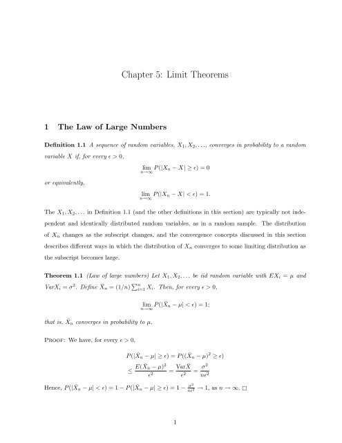
1 The Law of Large Numbers
Definition 1.1 A sequence of random variables, X 1 , X 2 , . . ., converges in probability to a random
variable X if, for every ɛ > 0,
or equivalently,
lim P (|X n − X| ≥ ɛ) = 0
n→∞
lim P (|X n − X| < ɛ) = 1.
n→∞
The X 1 , X 2 , . . . in Definition 1.1 (and the other definitions in this section) are typically not independent
and identically distributed random variables, as in a random sample. The distribution
of X n changes as the subscript changes, and the convergence concepts discussed in this section
describes different ways in which the distribution of X n converges to some limiting distribution as
the subscript becomes large.
Theorem 1.1 (Law of large numbers) Let X 1 , X 2 , . . . be iid random variable with EX i = µ and
VarX i = σ 2 . Define ¯X n = (1/n) ∑ n
i=1 X i. Then, for every ɛ > 0,
that is, ¯Xn converges in probability to µ.
lim P (| ¯X n − µ| < ɛ) = 1;
n→∞
Proof: We have, for every ɛ > 0,
P (| ¯X n − µ| ≥ ɛ) = P (( ¯X n − µ) 2 ≥ ɛ)
≤ E( ¯X n − µ) 2
ɛ 2
=
Var ¯X
ɛ 2
Hence, P (| ¯X n − µ| < ɛ) = 1 − P (| ¯X n − µ| ≥ ɛ) = 1 − σ2
nɛ 2
= σ2
nɛ 2
→ 1, as n → ∞. □
1

The law of large numbers (also known as the weak law of large numbers or WLLN) quite elegantly
states that under general conditions, the sample mean approaches the population mean as n → ∞.
A type of convergence that is stronger than convergence in probability is almost sure convergence.
This type of convergence is similar to pointwise convergence of a sequence of functions,
except that the convergence need not occur on a set with probability 0 (hence the “almost” sure).
EX A (Consistency of S 2 ) Suppose we have a sequence X 1 , X 2 , . . . of iid random variables with
EX i = µ and VarX i = σ 2 < ∞. If we define
using Chebychev’s Inequality, we have
S 2 n = 1
n − 1
n∑
(X i − ¯X n ) 2 ,
i=1
P (|S 2 − σ 2 | ≥ ɛ) ≤ E(S2 n − σ 2 ) 2
ɛ 2
= VarS2 n
ɛ 2 ,
and thus, a sufficient condition that S 2 n converges in probability to σ 2 is that VarS 2 n → 0 as
n → ∞.
EX B (Monte Carlo Integration) Suppose that we wish to calculate
I(f) =
∫ 1
0
f(x)dx
where the integration can not be done by elementary means.
The Monte Carlo method
works in the following way. Generate independent uniform random variables on [0, 1]—that
is, X 1 , . . . , X n —and compute
Î(f) = 1 n
n∑
f(X i ).
By the law of large numbers, this should be close to E[f(x)] = ∫ 1
0 f(x)dx.
i=1
2 Convergence in Distribution and the Central Limit Theorem
Definition 2.1 A sequence of random variables, X 1 , X 2 , . . ., converges in distribution to a random
variable X if
at all points x where F X (x) is continuous.
lim F X
n→∞ n
(x) = F X (x)
2

EX A (Maximum of uniforms) If X 1 , X 2 , . . . are iid uniform(0,1) and X (n) = max 1≤i≤n X i , let us
examine if X (n) converges in distribution.
As n → ∞, we have for any ɛ > 0,
P (|X n − 1| ≥ ɛ) = P (X (n) ≤ 1 − ɛ)
= P (X i ≤ 1 − ɛ, i = 1, . . . , n) = (1 − ɛ) n ,
which goes to 0. However, if we take ɛ = t/n, we then have
P (X (n) ≤ 1 − t/n) = (1 − t/n) n → e −t ,
which, upon rearranging, yields
P (n(1 − X (n) ) ≤ t) → 1 − e −t ;
that is, the random variable n(1−X (n) ) converges in distribution to an exponential(1) random
variable.
Moment-generating function are often useful for establishing the convergence of distribution
functions. We know from chapter 4 that a distribution function F n is uniquely determined by its
mgf, M n . The following theorem states that this unique determination holds for limit as well.
Theorem 2.1 (Continuity Theorem) Let F n be a sequence of cumulative distribution functions with
the corresponding moment-generating function M n . Let F be a cumulative distribution function with
the moment-generating function M. If M n (t) → M(t) for all t in an open interval containing zero,
then F n (x) → F (x) at all continuity points of F .
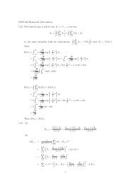
EX B We will show that the Poisson distribution can be approximated by the normal distribution
for large values of λ.
Let λ 1 , λ 2 , . . . be an increasing sequence with λ n → ∞, and let {X n } be a sequence of Poisson
random variables with the corresponding parameters. We know that E(X n ) = Var(X n ) = λ n .
Let
Z n = X n − λ n
√
λn
,
we then have E(Z n ) = 0 and Var(Z n ) = 1, and we will show that the mgf of Z n converges to
the mgf of standard normal distribution.
3

The mgf of X n is ψ Xn (t) = e λn(et −1) . The mgf of Z n is then
ψ Zn (t) = e −t√ λ n
t
ψ Xn ( √ )
λn
= e −t√ λ n
e λn(et/√ λn−1)
= e t2 2 + t3
3! √ λn +···.
Thus, lim n→∞ ψ Zn (t) = e t2 /2 , which concludes the proof.
EX C A certain type of particle is emitted at a rate of 900 per hour. What is the probability that
more than 950 particles will be emitted in a given hour if the counts form a Poisson process?
Let X be a Poisson random variable with mean 900. By Example B, we have
P (X > 950) = P ( X √ − 900 950 − 900
> √ ) ≈ 1 − Φ(5/3) = 0.04779.
900 900
For comparison, the exact probability is 0.04712.
Theorem 2.2 (Central limit theorem) Let X 1 , X 2 , . . . be a sequence of iid random variables whose
mgfs exist in a neighborhood of 0 (that is, M Xi (t) exists for |t| < h, for some positive h). Let
EX i = 0 and VarX i = σ 2 . Define S n = ∑ n
i=1 X i. Then, for any x, −∞ < x < ∞,
( )
lim P Sn
n→∞ σ √ n ≤ x = Φ(x).
Proof: Let Z n = S n /(σ √ n). We will show that the mgf of Z n tends to the mgf of the standard
normal distribution. Since S n is a sum of independent normal random variables,
and
ψ(s) has a Taylor expansion about zero:
ψ Sn (t) = [ψ(t)] n
ψ Zn (t) =
[ ( )] t
ψ
σ √ .
n
ψ(s) = ψ(0) + sψ ′ (0) + 1 2 s2 ψ ′′ (0) + ɛ s ,
where ɛ s /s 2 → 0 as s → 0. Since ψ ′ (0) = 0 and ψ ′′ (0) = σ 2 ,
( ) t
ψ
σ √ = 1 + 1 ( ) t 2
n 2 σ2 σ √ + ɛ n ,
n
where ɛ n /(t 2 /(nσ 2 )) → 0 as n → ∞. We thus have
) n
ψ Zn (t) =
(1 + t2
2n + ɛ n .
4

It can be shown that if a n → a, then
lim (1 + a n
n→∞ n )n = e a .
From this result, it follows that
ψ Zn (t) → e t2 /2 , as n → ∞,
which concludes the proof. □
The above theorem is one of the simplest versions of the central limit theorem; there are many
central limit theorems of various degrees of abdtraction and generality. We have proved the above
theorem under the assumption that the moment-generating function exist, which is a rather strong
assumption. The next theorem only requires that the first and second moments exist.
Theorem 2.3 (Stronger form of the central limit theorem) Let X 1 , X 2 , . . . be a sequence of iid
random variables with EX i = µ and 0 < VarX i = σ 2 < ∞. Define ¯X n = ( 1 n ) ∑ n
i=1 X i. Let G n (x)
denote the cdf of √ n( ¯X n − µ)/σ. Then, for any x, −∞ < x < ∞,
∫ x
lim G 1
n(x) = √ e −y2 /2 dy;
n→∞
−∞ 2π
that is, √ n( ¯X n − µ)/σ has a limiting standard normal distribution.
EX D Because the uniform distribution on [0, 1] has mean 1/2 and variance 1/12, the sum of 12
uniform random variables, minus 6, has mean 0 and variance 1. The distribution of this sum
is quite close to normal; in fact, before better algorithms were developed, it was commonly
used in computers for generating normal random variables from uniform ones.
Figure 5.1 shows a histogram of 1000 such sums with a superimposed normal density function.
EX E The sum of n independent random variables with parameter λ = 1 follows a gamma distribution
with λ = 1 and α = n. The exponential density is quite skewed; therefore, a good
approximation of a standardized gamma by a standardized normal would not be expected for
small n. Figure ?? shows that the approximation to normal improves as n increases.
EX F Since a binomial random variable is the sum of independent bernoulli random variables, its
is distribution can be approximated by a normal distribution. The approximation is best
when the binomial distribution is symmetric—that is, when p = 1/2.
A frequently used
5

Figure 1: A histogram of 1000 values, each of which is the sum of 12 uniform [−0.5, 0.5]
random variables.
Figure 2: The standard normal cdf (solid line) and the cdf’s of standardized gamma distributions
with α = 5 (log dashed), α = 10 (short dashed), and α = 30 (dots).
6

ule of thumb is that the approximation is reasonable when np > 5 and n(1 − p) > 5. The
approximation is especially useful for large values of n.
Suppose that a coin is tossed 100 times and lands heads up 60 times. Should we be supprised
and doubt that the coin is fair?
P (X ≥ 60) = P
( )
X − 50 100 − 50
√ ≥ √
25 25
≈ 1 − Φ(2)
= 0.0228
The probability is rather small, so the fairness of the coin is called into question.
7