Chapter 18: Split-Plot, Repeated Measures, and Crossover Designs

Chapter 18: Split-Plot, Repeated Measures, and Crossover Designs
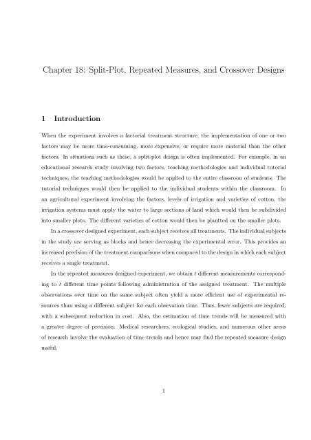
1 Introduction
When the experiment involves a factorial treatment structure, the implementation of one or two
factors may be more time-consuming, more expensive, or require more material than the other
factors. In situations such as these, a split-plot design is often implemented. For example, in an
educational research study involving two factors, teaching methodologies and individual tutorial
techniques, the teaching methodologies would be applied to the entire classroon of students. The
tutorial techniques would then be applied to the individual students within the classroom. In
an agricultural experiment involving the factors, levels of irrigation and varieties of cotton, the
irrigation systems must apply the water to large sections of land which would then be subdivided
into smaller plots. The different varieties of cotton would then be plantted on the smaller plots.
In a crossover designed experiment, each subject receives all treatments. The individual subjects
in the study are serving as blocks and hence decreasing the experimental error. This provides an
increased precision of the treatment comparisons when compared to the design in which each subject
receives a single treatment.
In the repeated measures designed experiment, we obtain t different measurements corresponding
to t different time points following administration of the assigned treatment. The multiple
observations over time on the same subject often yield a more efficient use of experimental resources
than using a different subject for each obsevation time. Thus, fewer subjects are required,
with a subsequent reduction in cost. Also, the estimation of time trends will be measured with
a greater degree of precision. Medical researchers, ecological studies, and numerous other areas
of research involve the evaluation of time trends and hence may find the repeated measure design
useful.
1

2 Split-Plot Designed Experiments
The yields of three different varieties of soybeans are to be compared under two different levels
of fertilizer application. If we are interested in getting n = 2 observations at each combination of
fertilizer and variety of soybeans, we would need 12 equal-sized plots. Taking fertilizer as factor A
and varieties as a treatment factor T, one possible design would be an 2 × 3 factorial treatment
structure with n = 2 observations per factor-level combination. However, since the application of
fertilizer to a plot occurs when the soil is being prepared for planting, it would be difficult to first
apply fertilizer A 1 to six of the plots dictated by the factorial arrangement of factors A and T and
then fertilizer A 2 to the other six plots before planting the required varieties of soybeans in each
plot.
An easier design to execute would have each fertilizer applied to two larger “wholeplots” and
then the varieties of soybeans planted in three “subplots” within each whole plot.
This design is called a split-plot design, and with this design there is a two-stage randomization.
First, levels of factor A (fertilizers) are randomly assigned to the wholeplots; second, the levels of
factor T (soybeans) are randomly assigned to the subplots within a wholeplot. Using this design,
it would be much easier to prepare the soil and to apply the fertilizer to the larger wholeplots.
Consider the model for the split-plot design with a levels of factor A, t levels of factor T, and
n repetitions of the i levels of factor A. If y ijk denotes the kth response for the ith level of factor
A, jth level of factor T, then
y ijk = µ + τ i + δ ik + γ j + τγ ij + ɛ ijk ,
where
• τ i : Fixed effect for ith level of A.
• γ j : Fixed effect for jth level of T.
• τγ ij : Fixed effect for ith level of A, jth level of T.
• δ ik : Random effect for the kth wholeplot receiving the ith level of A. The δ ik are independent
normal with mean 0 and variance σδ 2.
• ɛ ijk : Random error.
The δ ik and ɛ ijk are mutually independent.
2

Table 1: An ANOVA table for a completely randomized split-plot design.
Source SS df EMS
A SSA a − 1 σɛ 2 + tσδ 2 + tnθ τ
Wholeplot Error SS(A) a(n − 1) σɛ 2 + tσδ
2
T SST t − 1 σɛ 2 + anθ γ
AT SSAT (a − 1)(t − 1) σɛ 2 + nθ τγ
subplot error SSE a(n − 1)(t − 1) σɛ
2
Total TSS atn − 1
The ANOVA for this model and design is shown in Figure 1.
The sum of squares can be
computed using our standard formulas.
Wholeplot analysis
H 0 : θ τ = 0 (or, equivalently, H 0 : all τ i = 0), F = MSA
MS(A) .
Subplot Analysis
H 0 : θ τγ = 0 (or, equivalently, H 0 : All τγ ij = 0), F = MSAT
MSE .
H 0 : θ γ = 0 (or, equivalently, H 0 : All γ j = 0), F = MST
MSE .
A variation on this design introduces a blocking factor (such as farms). Thus for our example,
there may be b = 2 farms with a = 2 wholeplots per farm and t = 3 subplots per wholeplot. The
model for this more general two-factor split-plot design laid off in b blocks is as follows:
y ijk = µ + τ i + β j + τβ ij + γ k + τγ ik + ɛ ijk ,
where y ijk denotes the measurement receiving the ith level of factor A and the kth level of factor
T in the jth block. The parameters τ i , γ k , and τγ ik are the usual main effects and interaction
parameters for a two-factor experiment, whereas β j is the effect due to block j and τβ ij is the
interaction between the ith level of factor A and the jth block. The analysis corresponding to this
model is shown in Table 2.
• Wholeplot analysis.
H 0 : θ τ = 0 (or, equivalently, H 0 : all τ i = 0), F = MSA
MSAB .
• Subplot analysis.
H 0 : θ τγ = 0 (or, equivalently, H 0 : all τγ ik = 0), F = MSAT
MSE .
H 0 : θ γ = 0 (or, equivalently, H 0 : all γ k = 0), F = MST
MSE .
3

Table 2: An ANOVA table for a randomized split-plot design (A, T fixed; block random.
Source SS df EMS
Blocks SSB b − 1 σɛ 2 + atσβ
2
A SSA a − 1 σɛ 2 + tστβ 2 + btθ τ
AB(Wholeplot Error) SSAB (a − 1)(b − 1) σɛ 2 + tστβ
2
T SST t − 1 σɛ 2 + abθ γ
AT SSAT (a − 1)(t − 1) σɛ 2 + bθ τγ
subplot error SSE a(b − 1)(t − 1) σɛ
2
Total TSS abt − 1
Example 2.1 Soybeans are an important crop throughout the world. A study was designed to
determine if additional phosphorus applied to the soil would increase the yield of soybean. There
are three major varieties of soybeans of interest (V 1 , V 2 , V 3 ) and four levels of phosphorus (0, 20,
40, 65, pounds per acre). The researchers have nine plots of land available for the study which
are grouped into blocks of three plots each based on the soil characteristics of the plots. Because
of the complexities of planting the soybeans on plots of the given size, it was decided to plant a
single variety of soybeans on each plot and then divide each plot into four subplots. The researchers
randomly assigned a variety to one plot within each block of three plots and then randomly assigned
the levels of phosphorus to the four subplots within each plot. The yields (bushels/acre) froom the
36 plots are given in Table 18.5 of the textbook.
For this study, we have a randomized complete block design with a split-plot structure. Variety,
with 3 levels, is the wholeplot treatment and amount of phosphorus is the split-plot treatment. The
ANOVA analysis is as follows.
The results indicate that there is a significant variety by phosphorus interaction from which we
can conclude that the relationship between average yield and amount of phosphorus added to the
soil is not the same for the three varieties.
The distinction between this two-factor split-plot design and the standard two-factor experiments
discussed in Chapter 14 lies in the randomization. In a split-plot design, there are two stages
to the randomization process; first levels of factor A are randomized to the wholeplots within each
block, and then levels of factor B are randomized to the subplot units within each wholeplot of
every block. In contrast, for a two-factor experiment laid off in a randomized block design, the
4

Table 3: An ANOVA table for a randomized split-plot design (A, T fixed; block random).
Source df SS MS F p-value
Blocks 2 763.25 381.63 * *
V 2 671.81 335.90 232.60 < .0001
BV(Wholeplot Error) 4 6.56 1.64 * *
P 3 408.37 136.12 601.04 < 0.0001
PV 6 117.41 19.57 86.40 < 0.0001
subplot error 18 4.08 0.23
Total 35 1971.48
randomization is a one-step procedure; treatments (factor-level combinations of the two factors)
are randomized to the experimental units in each block.
5

3 Single-Factor Experiments with Repeated Measures
In Section 18.1, we discussed some reasons why one might want to get more than one observation
per patient. Consider a design, three compounds are administered in sequence to each of the n
patients. A compound is administered to a patient during a given treatment period. After a
sufficiently long “washout” period, another compound is given to the same patient. This procedure
is repeated until the patient has been treated with all three compounds. The order in which the
compounds are administered would be randomized. The data is shown below.
multicolumn4cPatient
Compound 1 2 · · · n
1 y 11 y 12 · · · y 1n
2 y 21 y 22 · · · y 2n
3 y 31 y 32 · · · y 3n
The model for this experiment can be written as
y ij = µ + τ i + δ j + ɛ ij ,
where µ is the overall mean response, τ i is the effect of the ith compound, δ j is the effect of jth
patient, and ɛ ij is the experimental error for the jth patient receiving the ith compound.
For this model, we make the following assumptions:
1. τ i s are constants with τ a = 0.
2. The δ j are independent and normally distributed N(0, σδ 2).
3. The ɛ ij s are independent of the δ j s.
4. The ɛ ij s are normally distributed N(0, σɛ 2 ).
5. The ɛ ij s have the following correlation relationship: ɛ ij and ɛ i ′ j are correlated for i ≠ i ′ ; and
ɛ ij and ɛ i ′ j ′ are independent for j ≠ j′ .
That is, two observations from the same patient are correlated but observations from different
patients are independent. From these assumptions it can be shown that the variance of y ij is
σδ 2 + σ2 ɛ . A further assumption is that the covariance for any two observations from patient j,
y ij and y i ′ j, is constant. These assumptions give rise to a variance-covariance matrix for the
observations, which exhibits compound symmetry.
6

The ANOVA table for the experiment is shown below.
Source SS df EMS (A fixed, patients random)
Patients SSP n − 1 σɛ 2 + aσδ
2
A SSA a − 1 σɛ 2 + nθ τ
Error SSE (a − 1)(n − 1) σɛ
2
Totals TSS an − 1
When the assumptions hold, and hence compound symmetry holds, the statistical test on factor
A (F = MSA/MSE) is appropriate. The conditions under which the F test for factor A is valid
are often not met because observations on the same patient taken closely in time are more highly
correlated than are observations taken farther apart in time. So be careful about this.
In general, when the variance-covariance matrix does not follow a pattern of compound symmetry,
the F test for factor A has a positive bias, which allows rejection of H 0 : all τ i = 0 more
often than is indicated by the critical F -value.
Example 3.1 An exercise physiologist designed a study to evaluate the impact of the steepness of
running courses on the peak heart rate (PHR) of well-conditioned runners. There are four five-mile
courses that have been rated as flat, slightly steep, moderately steep, and very steep with respect to
the general steepness of the terrain. The 20 runners will run each of the four courses in a randomly
assigned order. There will be sufficient time between the runs so that there should not be any
carryover effect and the weather conditions during the runs were essentially the same. Therefore,
the researcher felt confident that the model
y ij = µ + τ i + δ j + ɛ ij
would be appropriate for the experiment.
The ANOVA table for the experiment is shown below:
Source SS df EMS (A fixed, patients random) F Prob
Runner 4048.44 19 213.08 11.21 < 0.0001
Course 3619.25 3 1206.41 63.47 < 0.0001
Error 1083.51 57 19.01
Totals 8751.19 79
7

From the output we have that the p-value associated with the F test of
H 0 : µ 1 = µ 2 = µ 3 = µ 4 versus H 1 : not H 0
has p-value< 0.0001. Thus, we conclude that there is significant evidence of a difference in the
mean heart rates over the four levels of steepness.
The estimated variance components are given by
ˆσ 2 Error = MSE = 19.01
ˆσ 2 Runner = MS Runner − MSE
4
=
213.08 − 19.01
4
= 48.52
Therefore, 72% of the variation in the heart rates was due to the differences in runners and 28%
was due to all other sources.
8

4 Two-factor Experiments with Repeated Measures on One of the
Factors
We can extend our discussion of repeated measures experiments to two-factor settings. For example,
in comparing the blood-pressure-lowering effects of cardiovascular compounds, we could
randomize the patients so that n different patients receive each of the three compounds. Repeated
measurements occur due to taking multiple measurements across time for each patient. For example,
we might be interested in obtaining blood pressure readings immediately prior to receiving a
single dose of the assigned and then every 15 minutes for the first hour and hourly thereafter for
the next 6 hours.
This experiment can be described generally as follows. There are m treatments with n experimental
units randomly assigned to the treatments. Each experimental unit (EU) is assigned to a
single treatment with t measurements taken on each of the EUs. The form of the data is shown
below. Note that this is a two-factor experiment (treatment and time) with repeated measurements
taken over the time factor.
Time Period
Treatment EU 1 2 · · · t
1 1 y 111 y 112 · · · y 11t
. · · · · · · · · · · · ·
n y 1n1 y 1n2 · · · y 1nt
.
m 1 y m11 y m12 · · · y m1t
. · · · · · · · · · · · ·
n y mn1 y mn2 · · · y mnt
The analysis of a repeated measurement design can, under certain conditions, be approximated
by the methods used in a split-plot experiment.
• Each treatment is randomly assigned to an EU. This is the wholeplot in the split-plot design.
• Each EU is then measured at t time points. This is considered the split-plot unit.
• The major difference is that in a split-plot design, the levels of factor B are randomly assigned
to the split-plot EUs. In the repeated measurement design, the second randomization does
9

not occur, and thus there may be strong correlation between the measurements across time
made on the same EU.
The split-plot analysis is an appropriate analysis for a repeated measurement experiment only
when the covariance matrix of the measurements satisfy a particular type of structure: Compound
Symmetry:
⎧
σɛ ⎪⎨
when i = i ′ , j = j ′
Cov(y ijk , y i ′ j ′ k) = ρσɛ 2 when i = i ′ , j ≠ j ′
⎪⎩ 0 when i ≠ i ′
where y ijk is the measurement from the kth EU receiving treatment i at time j. Thus we have
Corr(y ijk , y ij ′ k) = ρ.
This implies that there is a constant correlation between observations no matter how far apart
they are taken in time. This may not be realistic in many applications. One would think that
observations in adjacent time periods would be more highly correlated than observations taken two
or three time periods apart.
The model can be written as
y ijk = µ + τ i + d ik + β j + (τβ) ij + ɛ ijk
where i = 1, . . . , m, j = 1, . . . , t, k = 1, . . . , n, τ i is the ith treatment effect, β j is the jth time
effect, (τβ) ij is the treatment-time interaction effect, d ik is the subject-treatment interaction effect
(random, independent, N(0, σd 2), ɛ ijk independent N(0, σɛ 2 ), and d ik and ɛ ijk are independently
distributed.
Let λ = tρ/2(1 − ρ). The ANOVA table for the split-plot analysis of a repeated measures
experiment is given in Table 4, where the treatment and time effects are fixed.
Based on Table 4, the following tests can be performed:
• H 0 : θ τβ = 0
• H 0 : θ β = 0
F = MS trt∗time
MSE
F = MS time
MSE
10

Table 4: An ANOVA table for a two-factor experiment, repeated measures on one factor.
Source df Expected Mean Squares
TRT m − 1 σɛ 2 (1 + 2λ) + tσd 2 + ntθ τ
EU(TRT) (n − 1)m σɛ 2 (1 + 2λ) + tσd
2
Time t − 1 σɛ 2 + nmθ β
TRT*Time (m − 1) ∗ (t − 1) σɛ 2 + nθ τβ
Error m(t − 1)(n − 1) σɛ
2
Total mnt − 1
• H 0 : θ τ = 0
F =
MS T rt
MS EU(trt)
Example 4.1 In a study, three levels of a vitamin E supplement, zero (control), low, and high,
were given to guinea pigs. Five pigs were randomly assigned to each of the three levels of the vitamin
E supplement. The weights of the pigs were recorded at 1, 2, 3, 4, 5, and 6 weeks after the beginning
of the study. This is a repeated measurement experiment because each pig, the EU, is given only
one treatment but each pig is measured six times.
The ANOVA table for the example is as follows.
Source df SS MS F p-value
TRT 2 18548.07 9274.03 1.06 0.3782
PIG(TRT) 12 105,434.20
Week 5 142,554.50 28510.90 52.55 < 0.0001
TRT*Week 10 9762.73 976.27 1.80 0.0801
Error 60 32,552.60 542.54
From this table, we find that there is not significant evidence of an interaction between the
treatment and time factors.
Since the interaction was not significant, the main effects of treatment and time can be analyzed
separately. The p-value=0.3782 for treatment differences and p-value< 0.0001 for time differences.
The mean weights of the pigs vary across the 6 weeks but there is not significant evidence of a
difference in the mean weights for the three levels of vitamin E feed supplements. Therefore, the
11

two levels of vitamin E supplement do not appear to provide an increase in the mean weights of
the pigs in comparison to the control, which was a zero level of vitamin E supplement.
12

5 Crossover Designs
In a crossover design, each experimental unit (EU) is observed under each of the t treatments
during t observation times. It is important to emphasize the difference between a crossover design
and the general repeated measurement design. In a repeated measurement design, the EU receives
receives a treatment and then the EU has multiple observations or measurements made on it over
time or space. The EU does not receive a new treatment between successive measurements.
The crossover designs are often useful when a latin square is to be used in a repeated measurement
study to balance the order positions of treatments, yet more subjects are required than
called for by a single latin square. With this type of design, the subjects are randomly assigned to
the different treatment order patterns given by a latin square. Consider an experiment in which
treatments A, B, and C are to be administered to each subject, and the three treatment order
pattern are given by the latin square
Order Position
pattern 1 2 3
1 A B C
2 B C A
3 C A B
Suppose that 3n subjects are available for the study. Then n subjects will be assigned at
random to each of the three order patterns in a latin square crossover design. Note that this design
is a mixture of repeated measures (within subjects) and latin square (order patterns from a latin
square).
For this experiment, the model can be written as
y ijkm = µ + ρ i + κ j + τ k + η m(i) + ɛ ijkm ,
where i = 1, . . . , t, j = 1, . . . , t, k = 1, . . . , t, and m = 1, . . . , m. The term ρ i denotes the effect
of the ith treatment order pattern, κ j denotes the effect of the jth order position, τ k denotes the
effect of the kth treatment, and η m(i) denotes the effect of subject m which is nested within the ith
treatment order pattern. Here we assume η m(i) are independent N(0, ση), 2 ɛ ijkm are independent
N(0, σɛ 2 ) and independent of the η m(i) .
The ANOVA table for the experiment is as follows.
13

Source of Variation SS df EMS
Patterns(P) SSP t − 1 σɛ 2 + rση 2 + nrθ ρ
Order Position(O) SSO t − 1 σɛ 2 + nrθ κ
Treatments(TR) SSTR t − 1 σɛ 2 + nrθ τ
Subjects SSS t(n − 1) σɛ 2 + rση
2
Error SSE (t − 1)(nt − 2) σɛ
2
Total SST nt 2 − 1
The formulas for the sums of squares follow the usual pattern:
SST = ∑ i
∑ ∑
(y ijkm − ȳ ... ) 2
j m
SSP = nt ∑ i
SSO = nt ∑ j
(ȳ i... − ȳ .... ) 2
(ȳ .j.. − ȳ .... ) 2
SST R = nt ∑ k
(ȳ ..k. − ȳ .... ) 2
SSS = t ∑ i
∑
(ȳ i..m − ȳ .... ) 2
m
SSE = SST − SSP − SSO − SST R − SSS.
Example 5.1 The following table contains data for a study of three different displays on the sale
of apples, using a latin square crossover design. Six stores were used, with two assigned at random
to each of the three treatment order patterns shown. Each display was kept for two weeks, and the
observed variable was sales per 100 customers.
Two-week Period(j)
Pattern(i) Store 1 2 3
1 m=1 9(B) 12(C) 15(A)
m=2 4(B) 12(C) 9(A)
2 m=1 12(A) 14(B) 3(C)
m=2 13(A) 14(B) 3(C)
3 m=1 7(C) 18(A) 6(B)
m=2 5(C) 20(A) 4(B)
The ANOVA table for the data is as follows:
14

The test for the treatment effect is
Source of Variation SS df MS
Patterns 0.33 2 0.17
Order positions 233.33 2 116.67
Displays 189.00 2 94.50
Stores (within patterns) 21.00 3 7.00
Error 20.33 8 2.54
F = MST R
MSE = 94.50
2.54 = 37.2
which is greater than F 0.05,2,8 = 4.46. Therefore, we conclude that there are differential sales effects
for the three displays. Tests for pattern effects, order position effects, and store effects were also
carried out. They indicated that order position effects were present, but no pattern or store effects.
Order position effects here are associated with the three time periods in which the displays were
studied, and may reflect seasonal effects as well as the results of special events, such as unusually
hot weather in one period.
If the order position effects are not approximately constant for all subjects (stores, etc.), a
crossover design is not fully effective. It may then be preferable to place the subjects into homogeneous
groups with respect to the order position effects and use independent latin squares for each
group.
Carryover Effects If carryover effects from one treatment to another are anticipated, that is, if
not only the order position but also the preceding treatment has an effect, these carryover effects
may be balanced out by choosing a latin square in which every treatment follows every other
treatment an equal number of times. For t = 4, an example of such a latin square is
Period
Subject 1 2 3 4
1 A B D C
2 B C A D
3 C D B A
4 D A C B
15

Note that treatment A follows each of the other treatments once, and similarly for the other
treatments. This design is appropriate when the carryover effects do not persist for more than one
period.
When t is odd, the sequence balance can be obtained by using a pair of latin squares with the
property that the treatment sequences in one square are reversed in the other square.
For the earlier apple display illustration in which three displays were studied in six stores, the
two latin squares might be as shown in the next table. The stores should first be placed into two
homogeneous groups and these should then be assigned to the two lattin squares.
Two-week Period(j)
Square Store 1 2 3
1 A B C
1 2 B C A
3 C A B
4 C B A
2 5 A C B
6 B A C
6 Research Study: Effects of Oil Spill and Plant Growth
On January 7, 1992, an underground oil pipline ruptured and caused the contamination of a marsh
along the Chiltipin Creek in San Patricio County, Texas. The cleanup process consisted of burning
the contaminated regions in the marsh. To evaluate the influence of the oil spill on the flora,
the researchers concentrated their findings with respect to Distichlis Spicata, a flora of particular
importance to the area of the spill. Two questions of importance to the researchers were as follows:
1. Did the oil site recover after the spill and burning?
2. How long did it take for the recovery?
At both the oil spill site and the control site 20 tracts were randomly chosen. After a 9-month
transition period, measurements were taken at approximately 3-month intervals for a total of 8 time
periods. During each time period, the number of Distichlis spicata within each of the 40 tracts was
recorded. The resulting ANOVA table is as follows.
16

Table 5: ANOVA for research study: Effects of oil spill on plant growth.
Source SS df MS F p-value
Treatment 10511.11 1 10511.11 6.56 0.0045
Tracts in treatment 60844.63 38 1601.17
Date 2845.09 7 406.44 19.35 0.0001
Date×treatment 602.29 7 86.04 4.01 0.0001
Error 5587.88 266 21.01
17