Solving Einstein's Equations the Generalized Harmonic Way

Solving Einstein’s Equations 

the Generalized Harmonic Way 

Lee Lindblom 

Caltech 

Collaborators: Larry Kidder, Keith Matthews, 

Robert Owen, Harald Pfeiffer, Oliver Rinne, 

Mark Scheel, Bela Szilagyi, Saul Teukolsky 

Center for Computational Relativity and Gravitation Seminar, 

Rochester Institute of Technology, October 17, 2008 

Lee Lindblom (Caltech) GH Einstein CCRG-RIT – 10/17/2008 1 / 34

Outline of Talk: 

Methods of Specifying Gauge (Coordinates). 

Generalized Harmonic (GH) Einstein Equations. 

Constraint Damping. 

Boundary Conditions. 

Constraint Preserving. 

Physical. 

Moving Black Holes in a Spectral Code. 

Dual Coordinate Frame Evolution. 

Choosing Coordinates by Feedback Control. 

Gauge Drivers in the GH Einstein System. 


Traditional ADM Gauge Conditions 

Construct a foliation of 

spacetime by spatial 

slices. 

Choose a time function 

with t = const. on these 

slices. 

Choose spatial coordinates, 

x k , on each slice. 

⃗n = ∂ τ 

(t, x k ) 

Decompose the 4-metric ψ ab into its 3+1 parts: 

ds 2 = ψ ab dx a dx b = −N 2 dt 2 + g ij (dx i + N i dt)(dx j + N j dt). 

The lapse N and shift N i measure how coordinates are laid out on 

spacetime: ⃗n = ∂ τ = ∂t 

∂τ ∂ t + ∂x k 

∂τ ∂ k, 

= 1 N ∂ t − Nk 

N ∂ k. 

Spacetime coordinates are determined in the traditional ADM 

method by specifying the lapse N and shift N i . 

∂ k 

(t + δt, x k ) 

Lee Lindblom (Caltech) GH Einstein CCRG-RIT – 10/17/2008 3 / 34 

∂ t

ADM Evolution System 

When the gauge is determined by specifying the lapse N and shift 

N k , the Einstein system becomes a set of evolution equations for 

the spatial metric g ij and extrinsic curvature K ij : 

∂ t g ij − N k ∂ k g ij = −2NK ij + ∇ i N j + ∇ j N i , 

( ) 

∂ t K ij − N k ∂ k K ij = N (3) 

R ij − 2K k i K kj + KK ij 

−∇ i ∇ j N + K ik ∂ j N k + K kj ∂ i N k . 

The Einstein equations also include constraints: 

0 = Mˆt 

≡ (3) R − K ij K ij + K 2 , 

0 = M i ≡ ∇ k K ki − ∇ i K . 

This traditional form of the Einstein equations is not hyperbolic, 

and numerical solutions are found to suffer from generic constraint 

violating instabilities. 


Generalized Harmonic Gauge Conditions 

An alternate way to specify the gauge (i.e. coordinates) in the 

Einstein equations is through the gauge source function H a : 

Let H a denote the function obtained by the action of the covariant 

scalar wave operator on the coordinates x a : 

H a ≡ ∇ c ∇ c x a = ψ bc (∂ b ∂ c x a − Γ e bc∂ e x a ) = −Γ a , 

where Γ a = ψ bc Γ a bc and ψ ab is the 4-metric. 


Generalized Harmonic Gauge Conditions 

An alternate way to specify the gauge (i.e. coordinates) in the 

Einstein equations is through the gauge source function H a : 

Let H a denote the function obtained by the action of the covariant 

scalar wave operator on the coordinates x a : 

H a ≡ ∇ c ∇ c x a = ψ bc (∂ b ∂ c x a − Γ e bc∂ e x a ) = −Γ a , 

where Γ a = ψ bc Γ a bc and ψ ab is the 4-metric. 

Specifying coordinates by the generalized harmonic (GH) method 

can be accomplished by choosing a gauge-source function 

H a (x, ψ), and requiring that 

(√ ) 

H a (x, ψ) = −Γ a = ∂ b −ψψ 

ab 

/ √ −ψ. 


Einstein’s Equation with the GH Method 

The spacetime Ricci tensor can be written as: 

R ab = − 1 2 ψcd ∂ c ∂ d ψ ab + ∇ (a Γ b) + F ab (ψ, ∂ψ), 

where ψ ab is the 4-metric, and Γ a = ψ bc Γ abc . 

The Generalized Harmonic Einstein equation is obtained by 

replacing Γ a with −H a (x, ψ) = −ψ ab H b (x, ψ): 

R ab − ∇ (a 

[ 

Γb) + H b) 

] 

= − 

1 

2 ψcd ∂ c ∂ d ψ ab − ∇ (a H b) + F ab (ψ, ∂ψ). 

The vacuum GH Einstein equation, R ab = 0 with Γ a + H a = 0, is 

therefore manifestly hyperbolic, having the same principal part as 

the scalar wave equation: 

0 = ∇ a ∇ a Φ = ψ ab ∂ a ∂ b Φ + F(∂Φ). 


Gauge and Constraints in Electromagnetism 

The usual representation of the vacuum Maxwell equations split 

into evolution equations and constraints: 

∂ t 

⃗ E = ⃗ ∇ × ⃗ B, ∇ · ⃗ E = 0, 

∂ t 

⃗ B = − ⃗ ∇ × ⃗ E, ∇ · ⃗ B = 0. 

These equations are often written in the more compact 

4-dimensional notation: ∇ a F ab = 0 and ∇ [a F bc] = 0, 

where F ab has components ⃗ E and ⃗ B. 





∂ t 

⃗ E = ⃗ ∇ × ⃗ B, ∇ · ⃗ E = 0, 

∂ t 

⃗ B = − ⃗ ∇ × ⃗ E, ∇ · ⃗ B = 0. 




Maxwell’s equations are often re-expressed in terms of a vector 

potential F ab = ∇ a A b − ∇ b A a : 

∇ a ∇ a A b − ∇ b ∇ a A a = 0. 





∂ t 

⃗ E = ⃗ ∇ × ⃗ B, ∇ · ⃗ E = 0, 

∂ t 

⃗ B = − ⃗ ∇ × ⃗ E, ∇ · ⃗ B = 0. 




Maxwell’s equations are often re-expressed in terms of a vector 

potential F ab = ∇ a A b − ∇ b A a : 

∇ a ∇ a A b − ∇ b ∇ a A a = 0. 

This form of Maxwell’s equations is manifestly hyperbolic as long 

as the gauge is chosen correctly, e.g., let ∇ a A a = H(x, t), giving: 

∇ a ∇ a A b ≡ ( −∂ 2 t + ∂ 2 x + ∂ 2 y + ∂ 2 z 

) 

Ab = ∇ b H. 


Constraint Damping 

Where are the constraints: ∇ a ∇ a A b = ∇ b H? 




Gauge condition becomes a constraint: 0 = C ≡ ∇ a A a − H. 

Maxwell’s equations imply that this constraint is preserved: 

∇ a ∇ a C = 0. 




Gauge condition becomes a constraint: 0 = C ≡ ∇ a A a − H. 

Maxwell’s equations imply that this constraint is preserved: 

∇ a ∇ a C = 0. 

Modify evolution equations by adding multiples of the constraints: 

∇ a ∇ a A b = ∇ b H+γ 0 t b C = ∇ b H+γ 0 t b (∇ a A a − H). 

These changes also affect the constraint evolution equation, 

∇ a ∇ a C−γ 0 t b ∇ b C = 0, 

so constraint violations are damped when γ 0 > 0. 


Generalized Harmonic Evolution System 

Frans Pretorius wrote a very nice second order finite difference 

AMR code to solve the generalized harmonic Einstein equations: 

0 = R ab − ∇ (a Γ b) − ∇ (a H b) , 

= R ab − ∇ (a C b) , 

where C a = H a + Γ a . Unfortunately initial code was very unstable. 


Generalized Harmonic Evolution System 

Frans Pretorius wrote a very nice second order finite difference 

AMR code to solve the generalized harmonic Einstein equations: 

0 = R ab − ∇ (a Γ b) − ∇ (a H b) , 

= R ab − ∇ (a C b) , 

where C a = H a + Γ a . Unfortunately initial code was very unstable. 

Imposing coordinates using a GH gauge function profoundly 

changes the constraints. The GH constraint, C a = 0, where 

C a = H a + Γ a , 

depends only on first derivatives of the metric. The standard 

Hamiltonian and momentum constraints, M a = 0, are determined 

by the derivatives of the gauge constraint C a : 

M a ≡ 

[ 

R ab − 1 2 ψ abR 

] 

n b = 

[∇ (a C b) − 1 2 ψ ab∇ c C c 

] 

n b . 


Constraint Damping Generalized Harmonic System 

Pretorius (based on a suggestion from Gundlach, et al.) modified 

the GH system by adding terms proportional to the gauge 

constraints: 

[ 

0 = R ab − ∇ (a C b) + γ 0 n (a C b) − 1 2 ψ ab n c C c 

], 

where n a is a unit timelike vector field. Since C a = H a + Γ a 

depends only on first derivatives of the metric, these additional 

terms do not change the hyperbolic structure of the system. 


Constraint Damping Generalized Harmonic System 

Pretorius (based on a suggestion from Gundlach, et al.) modified 

the GH system by adding terms proportional to the gauge 

constraints: 

[ 

0 = R ab − ∇ (a C b) + γ 0 n (a C b) − 1 2 ψ ab n c C c 

], 

where n a is a unit timelike vector field. Since C a = H a + Γ a 

depends only on first derivatives of the metric, these additional 

terms do not change the hyperbolic structure of the system. 

Evolution of the constraints C a follow from the Bianchi identities: 

0 = ∇ c ∇ c C a −2γ 0 ∇ c[ n (c C a) 

] 

+ C c ∇ (c C a) − 1 2 γ 0 n a C c C c . 

This is a damped wave equation for C a , that drives all small 

short-wavelength constraint violations toward zero as the system 

evolves (for γ 0 > 0). 


First-Order Einstein Evolution System 

Introduce new fields Π ab and Φ iab representing the time and space 

derivatives of the metric ψ ab . 

Our code solves a first-order representation of the GH Einstein 

evolution system: 

∂ t ψ ab = −NΠ ab + N i Φ iab , 

∂ t Π ab − N k ∂ k Π ab + Ng ki ∂ k Φ iab + γ 2 N k ∂ k ψ ab ≃ 0, 

∂ t Φ iab − N k ∂ k Φ iab + N∂ i Π ab − γ 2 N∂ i Ψ ab ≃ 0. 

Violations of the additional constraint, C iab = Φ iab − ∂ i ψ ab , are 

suppressed on the timescale 1/γ 2 by this evolution system. 

This evolution system can be written very abstractly as: 

∂ t u α + A k α β(u)∂ k u β = F α (u), where u α = {ψ ab , Π ab , Φ iab }. 

This system is symmetric hyperbolic because there exists a 

positive definite symmetric S αβ that symmetrizes the 

characteristic matrices: A k αβ = Ak βα = S αγA k γ β. 


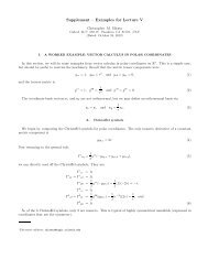
Numerical Tests of the First-Order GH System 

3D numerical evolutions of static black-hole spacetimes illustrate 

the constraint damping properties of the GH evolution system. 

These evolutions are stable and convergent when γ 0 = γ 2 = 1. 

|| C || 

10 -4 

10 -6 

10 -2 t/M 

γ 0 

= γ 2 

= 0.0 

γ 0 

= 1.0, 

γ 2 

= 0.0 

γ 0 

= 0.0, γ 2 

= 1.0 

|| C || 

10 -4 

10 -6 

10 -2 t/M 

{N r 

, L max 

} = {9, 7} 

{11, 7} 

10 -8 

γ 0 

= γ 2 

= 1.0 

10 -8 

{13, 7} 

10 -10 

0 100 200 

10 -10 

0 5000 10000 

The boundary conditions used for this simple test problem freeze 

the incoming characteristic fields to their initial values. 








Physical. 






Boundary Conditions 

Boundary conditions are straightforward to formulate for first-order 

hyperbolic evolutions systems, 

∂ t u α + A k α β(u)∂ k u β = F α (u). 

For the GH system u α = {ψ ab , Π ab , Φ kab }. 







Find the eigenvectors of the characteristic matrix s k A k α β at each 

boundary point: 

e ˆα α s k A k α β = v (ˆα) e ˆα β, 

where s k is the outward directed unit normal to the boundary. 











For hyperbolic evolution systems the eigenvectors e ˆα α are 

complete: det e ˆα α ≠ 0. So we define the characteristic fields: 

u ˆα = e ˆα αu α . 











For hyperbolic evolution systems the eigenvectors e ˆα α are 

complete: det e ˆα α ≠ 0. So we define the characteristic fields: 

u ˆα = e ˆα αu α . 

A boundary condition must be imposed on each incoming 

characteristic field (i.e. every field with v (ˆα) < 0), and must not be 

imposed on any outgoing field (i.e. any field with v (ˆα) > 0). 


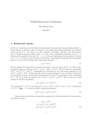
Evolutions of a Perturbed Schwarzschild Black Hole 

A black-hole spacetime is 

perturbed by an incoming 

gravitational wave that excites 

quasi-normal oscillations. 

Use boundary conditions that 

Freeze the remaining 

incoming characteristic fields. 

{N r 

, L } = 

{11, 9} 

10 -6 

|| C || 

{13, 11} 

10 -10 

{17, 15} 

{21, 19} 

10 -14 

0 50 100 

10 -2 max 

t/M 

The resulting outgoing waves 

interact with the boundary of 

the computational domain and 

produce constraint violations. 

Lapse Movie 

Constraint Movie 


Constraint Evolution for the First-Order GH System 

The evolution of the constraints, 

c A = {C a , C kab , M a ≈ n c ∂ c C a , C ka ≈ ∂ k C a , C klab = ∂ [k Φ l]ab } are 

determined by the evolution of the fields u α = {ψ ab , Π ab , Φ kab }: 

∂ t c A + A k A B(u)∂ k c B = F A B(u, ∂u) c B . 







This constraint evolution system is symmetric hyperbolic with 

principal part: 

∂ t C a ≃ 0, 

∂ t M a − N k ∂ k M a − Ng ij ∂ i C ja ≃ 0, 

∂ t C ia − N k ∂ k C ia − N∂ i M a ≃ 0, 

∂ t C iab − (1 + γ 1 )N k ∂ k C iab ≃ 0, 

∂ t C ijab − N k ∂ k C ijab ≃ 0. 







This constraint evolution system is symmetric hyperbolic with 

principal part: 

∂ t C a ≃ 0, 

∂ t M a − N k ∂ k M a − Ng ij ∂ i C ja ≃ 0, 

∂ t C ia − N k ∂ k C ia − N∂ i M a ≃ 0, 

∂ t C iab − (1 + γ 1 )N k ∂ k C iab ≃ 0, 

∂ t C ijab − N k ∂ k C ijab ≃ 0. 

An analysis of this system shows that all of the constraints are 

damped in the WKB limit when γ 0 > 0 and γ 2 > 0. So, this 

system has constraint suppression properties that are similar to 

those of the Pretorius (and Gundlach, et al.) system. 


Constraint Preserving Boundary Conditions 

Construct the characteristic fields, ĉÂ = eÂAc A , associated with 

the constraint evolution system, ∂ t c A + A k A B∂ k c B = F A Bc B . 





Split the constraints into incoming and outgoing characteristics: 

ĉ = {ĉ − , ĉ + }. 






ĉ = {ĉ − , ĉ + }. 

The incoming characteristic fields mush vanish on the boundaries, 

ĉ − = 0, if the influx of constraint violations is to be prevented. 






ĉ = {ĉ − , ĉ + }. 



The constraints depend on the primary evolution fields (and their 

derivatives). We find that ĉ − for the GH system can be expressed: 

ĉ − = d ⊥ û − + ˆF(u, d ‖ u). 






ĉ = {ĉ − , ĉ + }. 



The constraints depend on the primary evolution fields (and their 

derivatives). We find that ĉ − for the GH system can be expressed: 

ĉ − = d ⊥ û − + ˆF(u, d ‖ u). 

Set boundary conditions on the fields û − by requiring 

d ⊥ û − = −ˆF(u, d ‖ u). 


More Boundary Condition Issues 

Constraints can not provide BCs for all incoming fields. 

Physical gravitational-wave degrees-of-freedom must have BCs 

determined by the physics of the situation: 






Isolated systems (no incoming gravitational waves) are modeled by 

imposing a BC that sets the time-dependent part of the incoming 

components of the Weyl tensor to zero: ∂ t Ψ 0 = 0. 

This condition is translated into a BC by expressing Ψ 0 in terms of 

the incoming characteristic fields: Ψ 0 = d ⊥ û − + ˆF(u, d ‖ u). 











Initial-boundary problem for first-order GH evolution system is 

well-posed for algebraic boundary conditions on û α . 

Constraint preserving and physical boundary conditions involve 

derivatives of û α , and standard well-posedness proofs fail. 











Initial-boundary problem for first-order GH evolution system is 

well-posed for algebraic boundary conditions on û α . 

Constraint preserving and physical boundary conditions involve 

derivatives of û α , and standard well-posedness proofs fail. 

Oliver Rinne (2006) used Fourier-Laplace analysis to show that 

these BC satisfy the Kreiss (1970) condition which is necessary 

for well-posedness (but not sufficient for this type of BC). 


Numerical Tests of Boundary Conditions 

Compare the solution obtained on a “small” computational domain 

with a reference solution obtained on a “large” domain where the 

boundary is not in causal contact with the comparison region. 

Solution Differences 

Constraints 

Solutions using “Freezing” BC (dashed curves) have differences 

and constraints that do not converge to zero. 

Solutions using constraint preserving and physical BC (solid 

curves) have much smaller differences and constraints that 

converge to zero. 








Physical. 






Moving Black Holes in a Spectral Code 

Spectral: Excision boundary is a smooth analytic surface. 




Cannot add/remove individual grid points. 





Straightforward method: re-grid when holes move too far. 
















Problems: 

Re-gridding/interpolation is expensive. 






Problems: 


Difficult to get smooth extrapolation at trailing edge of horizon. 






Problems: 



Causality trouble at leading edge of horizon. 






Problems: 




t 

Horizon 

Outside 

Horizon 

x 






Problems: 




t 

Horizon 

Outside 

Horizon 

x 






Problems: 




Solution: 

t 

Choose coordinates that smoothly 

track the location of the black hole. 

For a black hole binary this means 

using coordinates that rotate with 

respect to inertial frames at infinity. 

Horizon 

Outside 

Horizon 

x 


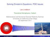
Evolving Black Holes in Rotating Frames 

Coordinates that rotate with respect to the inertial frames at 

infinity are needed to track the horizons of orbiting black holes. 

Evolutions of Schwarzschild in rotating coordinates are unstable. 

10 -8 Ω = 0.2/Μ 

10 -10 

|| C || 

10 -12 

10 -14 

Ω = 0.02/Μ 

Ω = 0.0002/Μ 

Ω = 0.002/Μ 

10 -5 10 -3 10 -1 10 1 10 3 

t / M 

Evolutions shown use a 

computational domain that 

extends to r = 1000M. 

Angular velocity needed to 

track the horizons of an equal 

mass binary at merger is 

about Ω ≈ 0.2/M. 

Problem caused by asymptotic 

behavior of metric in rotating 

coordinates: ψ tt ∼ ρ 2 Ω 2 , 

ψ ti ∼ ρΩ, ψ ij ∼ 1. 


Dual-Coordinate-Frame Evolution Method 

Single-coordinate frame method uses the one set of coordinates, 

x ā = {¯t, x ī}, to define field components, uᾱ = {ψā¯b, Πā¯b, Φīā¯b}, 

and the same coordinates to determine these components by 

solving Einstein’s equation for uᾱ = uᾱ(x ā): 

∂¯tuᾱ + A¯k ᾱ ¯β∂¯ku ¯β = F ᾱ. 







∂¯tuᾱ + A¯k ᾱ ¯β∂¯ku ¯β = F ᾱ. 

Dual-coordinate frame method uses basis vectors of one 

coordinate system to define components of fields, and a second 

set of coordinates, x a = {t, x i } = x a (x ā), to represent these 

components as functions, uᾱ = uᾱ(x a ). 







∂¯tuᾱ + A¯k ᾱ ¯β∂¯ku ¯β = F ᾱ. 

Dual-coordinate frame method uses basis vectors of one 

coordinate system to define components of fields, and a second 

set of coordinates, x a = {t, x i } = x a (x ā), to represent these 

components as functions, uᾱ = uᾱ(x a ). 

These functions are determined by solving the transformed 

Einstein equation: 

[ ∂x 

i 

∂ t uᾱ + 

∂¯t δᾱ ¯β + ∂x ] 

i 

A¯k ᾱ 

∂x ¯k ¯β ∂ i u ¯β = F ᾱ. 


Testing Dual-Coordinate-Frame Evolutions 

Single-frame evolutions of Schwarzschild in rotating coordinates 

are unstable, while dual-frame evolutions are stable: 

Dual Frame Evolution Single Frame Evolution 

N r 

= 9 

10 -8 Ω = 0.2/Μ 

10 -6 

|| C || 

10 -8 

N r 

= 11 

10 -10 

|| C || 

Ω = 0.02/Μ 

N r 

= 13 

Ω = 0.0002/Μ 

10 -10 N r 

= 15 

10 -12 

N r 

= 17 

Ω = 0.002/Μ 

10 -12 

0 200 400 600 800 1000 

10 -14 

10 -4 t / M 

Dual-frame evolution shown here uses a comoving frame with 

Ω = 0.2/M on a domain with outer radius r = 1000M. 

10 -5 10 -3 10 -1 10 1 10 3 

t / M 


Horizon Tracking Coordinates 

Coordinates must be used that track the motions of the holes. 

A coordinate transformation from inertial coordinates, (¯x, ȳ, ¯z), to 

co-moving coordinates (x, y, z), consisting of a rotation followed 

by an expansion, 

⎛ 

⎝ 

x 

y 

z 

⎞ 

⎛ 

⎠ = e a(¯t) ⎝ 

cos ϕ(¯t) − sin ϕ(¯t) 0 

sin ϕ(¯t) cos ϕ(¯t) 0 

0 0 1 

⎞ ⎛ 

⎠ ⎝ 

with t = ¯t, is general enough to keep the holes fixed in co-moving 

coordinates for suitably chosen functions a(¯t) and ϕ(¯t). 

Since the motions of the holes are not known a priori, the 

functions a(¯t) and ϕ(¯t) must be chosen dynamically and 

adaptively as the system evolves. 

¯x 

ȳ 

¯z 

⎞ 

⎠ , 


Horizon Tracking Coordinates II 

δϕ 

x 

c 

y 

c 

Measure the comoving centers of the holes: x c (t) and y c (t), or 

equivalently Q x (t) = [x c (t) − x c (0)]/x c (0) and Q y (t) = y c (t)/x c (t). 

Choose the map parameters a(t) and ϕ(t) to keep Q x (t) and 

Q y (t) small. 



δϕ 

x 

c 

y 

c 





Changing the map parameters by the small amounts, δa and δϕ, 

results in associated small changes in δQ x and δQ y : 

δQ x = −δa, 

δQ y = −δϕ. 



δϕ 

x 

c 

y 

c 





Changing the map parameters by the small amounts, δa and δϕ, 

results in associated small changes in δQ x and δQ y : 

δQ x = −δa, 

δQ y = −δϕ. 

Measure the quantities Q y (t), dQ y (t)/dt, d 2 Q y (t)/dt 2 , and set 

d 3 ϕ 

dt 3 = λ3 Q y + 3λ 2 dQ y 

+ 3λ d 2 Q y 

dt dt 2 = − d 3 Q y 

dt 3 . 

The solutions to this “closed-loop” equation for Q y have the form 

Q y (t) = (At 2 + Bt + C)e −λt , so Q y always decreases as t → ∞. 


Horizon Tracking Coordinates III 

In practice the coordinate maps are adjusted only at a prescribed 

set of adjustment times t = t i . 

In the time interval t i < t < t i+1 we set: 

ϕ(t) = ϕ i + (t − t i ) dϕ i 

( 

dt 

+ (t − t i) 3 

2 

λ d 2 Q y 

i 

dt 2 

+ (t − t i) 2 

2 

d 2 ϕ i 

dt 2 

+ λ 2 dQ y 

i 

dt 

+ λ 3 Q y 

i 

3 

where Q x , Q y , and their derivatives are measured at t = t i , so 

these maps satisfy the closed loop 

equation at t = t i . 

) 

, 


Horizon Tracking Coordinates III 

In practice the coordinate maps are adjusted only at a prescribed 

set of adjustment times t = t i . 

In the time interval t i < t < t i+1 we set: 

ϕ(t) = ϕ i + (t − t i ) dϕ i 

( 

dt 

+ (t − t i) 3 

2 

λ d 2 Q y 

i 

dt 2 

+ (t − t i) 2 

2 

d 2 ϕ i 

dt 2 

+ λ 2 dQ y 

i 

dt 

+ λ 3 Q y 

i 

3 

where Q x , Q y , and their derivatives are measured at t = t i , so 

2×10 

these maps satisfy the closed loop 

-4 Q y y c 

(t) 

= 

x 

equation at t = t i . 

c 

(t) 

This works! We are now able 

to evolve binary black holes using 

horizon tracking coordinates until 

just before merger. 

1×10 -4 

-1×10 -4 0 

Q x = 

) 

t / M ADM 

-2×10 -4 

0 1000 2000 3000 4000 

, 

x c 

(t) - x c 

(0) 

x c 

(0) 








Physical. 






Gauge Conditions and Hyperbolicity 

The GH Einstein equations may be written (abstractly) as 

ψ cd ∂ c ∂ d ψ ab = ∇ a H b + ∇ b H a + Q ab (ψ, ∂ψ). 

These equations are manifestly hyperbolic when H a is specified 

as a function of x a and ψ ab : H a = H a (x, ψ). 


Gauge Conditions and Hyperbolicity 

The GH Einstein equations may be written (abstractly) as 

ψ cd ∂ c ∂ d ψ ab = ∇ a H b + ∇ b H a + Q ab (ψ, ∂ψ). 

These equations are manifestly hyperbolic when H a is specified 

as a function of x a and ψ ab : H a = H a (x, ψ). 

Unfortunately, most gauge conditions found useful in numerical 

relativity are conditions on ψ ab and ∂ c ψ ab . 

The GH Einstein equations are typically not hyperbolic for gauge 

conditions of this type: H a = H a (x, ψ, ∂ψ). 


Solution: Gauge Driver Equations 

Elevate H a to the status of a dynamical field (Pretorius) and evolve 

it along with the spacetime metric ψ ab : 

Gauge Driver : ψ cd ∂ c ∂ d H a = Q a (x, H, ∂H, ψ, ∂ψ), 

GH Einstein : ψ cd ∂ c ∂ d ψ ab = Q ab (x, H, ∂H, ψ, ∂ψ). 

Any gauge driver of this form makes the combined 

Einstein–Gauge system hyperbolic. 









Choose Q a so that H a evolves toward the desired gauge target F a 

as the system evolves: H a → F a . 









Choose Q a so that H a evolves toward the desired gauge target F a 

as the system evolves: H a → F a . 

We have shown that the simple gauge driver: 

ψ cd ∂ c ∂ d H a = Q a = µ 2 (H a − F a ) + 2µN −1 ∂ t H a + ... 

drives H a → F a for some of the standard numerical relativity 

gauges: Phys. Rev. D 77 084001 (2008). 


Recent Gauge Driver Improvements 

Replace the wave operator in the gauge driver by a flat-space 

wave operator: 

η cd ∂ c ∂ d H a = Q a (x, H, ∂H, ψ, ∂ψ). 






Use improved boundary conditions for the gauge fields, e.g. 

∂ t H a = −µ(H a − F a ). 






Use improved boundary conditions for the gauge fields, e.g. 

∂ t H a = −µ(H a − F a ). 

The gauge field H a transforms like the trace of a connection. 

Evolutions done in a co-moving reference frame need an 

appropriate Hessian term added to F a : 

∂ 2 x b 

F a → F a − ψ ab 

∂x ¯b∂x ψ¯b¯c . ¯c 


Testing the Improved Gauge Driver System: 

Initial Data: use Schwarzschild with perturbed lapse and shift. 

Gauge Driver: use F a representing one of the Bona-Masso slicing 

conditions and one of the Γ-driver shift conditions. 

VMinusFNorm Sep12A 

10 0 

10 -2 Sep12A GhCe and VwCe 

|| C || 

|| H - F || / || F || 

10 -3 

10 -1 

10 -4 

10 -2 

10 -5 

t / M 

0 500 1000 1500 2000 

10 -3 

t / M 

0 500 1000 1500 2000 


In Progress: Binary Black Hole Evolutions 

Our gauge driver system is now robust enough to perform binary 

black hole evolutions. 

Which gauge conditions are both stable and effective for 

performing BBH mergers? 

BBH mergers have been performed using driver versions of the 

following gauge conditions, 

∂ t N − N k ∂ k N = −λNK , 

[ ] 

∂ t N i = ν 

(3)˜Γi − ηΥ i , 

∂ t Υ i + ηΥ i = (3)˜Γi . 


Summary 

Generalized Harmonic method produces manifestly hyperbolic 

representations of the Einstein equations for any choice of 

coordinates (when imposed in the appropriate way). 

Constraint damping makes the modified GH equations stable for 

numerical simulations. 

Constraint preserving and physical boundary conditions ensure 

that waves propagate through computational boundaries without 

(much) reflection. 

Dual coordinate frame evolution makes evolutions stable in 

coordinates that track the black hole motions. 

Feedback control systems can be used to construct co-moving 

coordinates that accurately track the black hole motions. 

Gauge drivers allow a wide range of useful gauge conditions in 

the generalized harmonic framework.

Solving Einstein's Equations the Generalized Harmonic Way

Create successful ePaper yourself

Delete template?

Save as template?