Gauge drivers for the generalized harmonic Einstein equations
Gauge drivers for the generalized harmonic Einstein equations
Gauge drivers for the generalized harmonic Einstein equations

Create successful ePaper yourself
Turn your PDF publications into a flip-book with our unique Google optimized e-Paper software.
PHYSICAL REVIEW D 77, 084001 (2008)<br />
<strong>Gauge</strong> <strong>drivers</strong> <strong>for</strong> <strong>the</strong> <strong>generalized</strong> <strong>harmonic</strong> <strong>Einstein</strong> <strong>equations</strong><br />
Lee Lindblom, 1 Keith D. Mat<strong>the</strong>ws, 1 Oliver Rinne, 1,2,3 and Mark A. Scheel 1<br />
1 Theoretical Astrophysics 130-33, Cali<strong>for</strong>nia Institute of Technology, Pasadena, Cali<strong>for</strong>nia 91125, USA<br />
2 Department of Applied Ma<strong>the</strong>matics and Theoretical Physics, Centre <strong>for</strong> Ma<strong>the</strong>matical Sciences,<br />
Wilber<strong>for</strong>ce Road, Cambridge CB3 0WA, United Kingdom<br />
3 King’s College, Cambridge CB2 1ST, United Kingdom<br />
(Received 13 November 2007; published 1 April 2008)<br />
The <strong>generalized</strong> <strong>harmonic</strong> representation of <strong>Einstein</strong>’s <strong>equations</strong> is manifestly hyperbolic <strong>for</strong> a large<br />
class of gauge conditions. Un<strong>for</strong>tunately most of <strong>the</strong> useful gauges developed over <strong>the</strong> past several<br />
decades by <strong>the</strong> numerical relativity community are incompatible with <strong>the</strong> hyperbolicity of <strong>the</strong> <strong>equations</strong> in<br />
this <strong>for</strong>m. This paper presents a new method of imposing gauge conditions that preserves hyperbolicity <strong>for</strong><br />
a much wider class of conditions, including as special cases many of <strong>the</strong> standard ones used in numerical<br />
relativity: e.g., K freezing, freezing, Bona-Massó slicing, con<strong>for</strong>mal <strong>drivers</strong>, etc. Analytical and<br />
numerical results are presented which test <strong>the</strong> stability and <strong>the</strong> effectiveness of this new gauge-driver<br />
evolution system.<br />
DOI: 10.1103/PhysRevD.77.084001 PACS numbers: 04.25.D , 02.60.Cb, 04.20.Cv, 04.25.dg<br />
I. INTRODUCTION<br />
The gauge (or coordinate) degrees of freedom in <strong>the</strong><br />
<strong>generalized</strong> <strong>harmonic</strong> (GH) <strong>for</strong>m of <strong>the</strong> <strong>Einstein</strong> <strong>equations</strong><br />
are determined by specifying <strong>the</strong> gauge source functions<br />
H a . These functions are defined as <strong>the</strong> results of <strong>the</strong><br />
covariant scalar-wave operator acting on each of <strong>the</strong> spacetime<br />
coordinates x a :<br />
H a r c r c x a : (1)<br />
The GH <strong>for</strong>m of <strong>the</strong> <strong>Einstein</strong> <strong>equations</strong> can be represented<br />
(somewhat abstractly) as<br />
cd @ c @ d ab @ a H b @ b H a Q ab H; ; @ ; (2)<br />
where ab is <strong>the</strong> spacetime metric, H a ab H b , and Q ab<br />
represents lower order terms that depend on H a , <strong>the</strong> metric,<br />
and its first derivatives.<br />
The GH <strong>for</strong>m of <strong>the</strong> <strong>Einstein</strong> <strong>equations</strong> is manifestly<br />
hyperbolic whenever H a is specified as an explicit function<br />
of <strong>the</strong> coordinates and <strong>the</strong> metric: H a H a x; . In this<br />
case <strong>the</strong> terms @ a H b that appear in Eq. (2) contain at most<br />
first derivatives of <strong>the</strong> metric. The <strong>Einstein</strong> <strong>equations</strong> become,<br />
<strong>the</strong>re<strong>for</strong>e, a set of second-order wave <strong>equations</strong> <strong>for</strong><br />
each component of <strong>the</strong> spacetime metric:<br />
cd @ c @ d ab<br />
^Q ab x; ; @ : (3)<br />
Thus <strong>the</strong> <strong>Einstein</strong> <strong>equations</strong> are manifestly hyperbolic <strong>for</strong><br />
any H a H a x; .<br />
Most of <strong>the</strong> useful gauge conditions developed by <strong>the</strong><br />
numerical relativity community over <strong>the</strong> past several decades<br />
cannot, un<strong>for</strong>tunately, be expressed in <strong>the</strong> simple <strong>for</strong>m<br />
H a H a x; (unless <strong>the</strong> full spacetime metric ab<br />
ab x is known a priori). Many of <strong>the</strong>se conditions<br />
(e.g., maximal slicing or <strong>drivers</strong>) would require gauge<br />
source functions that depend on <strong>the</strong> spacetime metric and<br />
its first derivatives: H a H a x; ; @ . In this case <strong>the</strong><br />
terms @ a H b in Eq. (2) depend on <strong>the</strong> second derivatives<br />
of <strong>the</strong> metric, ab , and this (generically) destroys <strong>the</strong><br />
hyperbolicity of <strong>the</strong> system.<br />
Pretorius [1–3] proposed a way to expand significantly<br />
<strong>the</strong> class of allowed gauge conditions, by elevating H a to<br />
<strong>the</strong> status of an independent dynamical field. A separate<br />
gauge-driver equation is introduced to evolve H a , <strong>for</strong><br />
example,<br />
r c r c H a Q a x; H; @H; ; @ ; (4)<br />
where r c r c H a denotes <strong>the</strong> wave operator 1 acting on H a .<br />
This gauge-driver equation is solved toge<strong>the</strong>r with <strong>the</strong> GH<br />
<strong>Einstein</strong> <strong>equations</strong> to determine ab and H a simultaneously.<br />
In <strong>the</strong> combined evolution system, consisting of<br />
Eqs. (2) and (4), <strong>the</strong> @ a H b terms in Eq. (2) are now lowerderivative<br />
terms that do not affect <strong>the</strong> hyperbolicity of <strong>the</strong><br />
system. Thus <strong>the</strong> combined GH <strong>Einstein</strong> plus gauge-driver<br />
system is manifestly hyperbolic so long as Q a on <strong>the</strong> right<br />
in Eq. (4) depends only on <strong>the</strong> fields and <strong>the</strong>ir first derivatives:<br />
Q a Q a x; H; @H; ; @ . Each of <strong>the</strong> solutions,<br />
H a H a x , to <strong>the</strong>se gauge-driver <strong>equations</strong> is a gauge<br />
condition. So <strong>the</strong> gauge-driver system provides a way <strong>for</strong><br />
H a to be determined by <strong>the</strong> metric and its derivatives in a<br />
flexible way without destroying <strong>the</strong> hyperbolicity of <strong>the</strong><br />
GH <strong>Einstein</strong> <strong>equations</strong>.<br />
Pretorius used a particular gauge-driver equation of this<br />
<strong>for</strong>m to determine H t in his ground breaking binary blackhole<br />
simulations:<br />
r c r c H t 1 1 N N p 2 @ t H t N k @ k H t N 1 ;<br />
(5)<br />
where in this case r c r c is <strong>the</strong> covariant scalar-wave<br />
operator, N is <strong>the</strong> lapse, N k is <strong>the</strong> shift, and 1 , 2, and p<br />
are constants. For suitable choices of <strong>the</strong>se parameters,<br />
1 We define exactly what we mean by this wave operator in<br />
Sec. II B.<br />
1550-7998=2008=77(8)=084001(17) 084001-1 © 2008 The American Physical Society
LINDBLOM et al. PHYSICAL REVIEW D 77, 084001 (2008)<br />
Pretorius found this system to be quite effective in preventing<br />
<strong>the</strong> lapse from ‘‘collapsing’’ toward zero as <strong>the</strong> system<br />
evolves. Solutions to this gauge driver do not correspond to<br />
any of <strong>the</strong> traditional gauge conditions of numerical relativity<br />
as far as we know.<br />
In this paper we introduce a new class of gauge-driver<br />
<strong>equations</strong> that are general enough to provide implementations<br />
of (almost) all of <strong>the</strong> standard gauge conditions used<br />
by <strong>the</strong> numerical relativity community. This is done by<br />
choosing an appropriate ‘‘source’’ term Q a <strong>for</strong> <strong>the</strong> right<br />
side of Eq. (4). The idea is to choose Q a so that solutions<br />
H a evolve quickly toward a target gauge source function<br />
F a . This F a is chosen so that strict equality H a F a<br />
corresponds exactly to <strong>the</strong> gauge condition of interest to<br />
us. We limit F a only by assuming that it depends on <strong>the</strong><br />
spacetime metric and its first (but not second) derivatives:<br />
F a F a x; ; @ . These new gauge-driver <strong>equations</strong> are<br />
introduced in Sec. II, and we show <strong>the</strong>re that <strong>the</strong> combined<br />
GH <strong>Einstein</strong> plus gauge-driver system is symmetric hyperbolic<br />
<strong>for</strong> any target gauge source function of this allowed<br />
<strong>for</strong>m. In Sec. III we present <strong>the</strong> target gauge functions F a<br />
corresponding to (many of) <strong>the</strong> gauge conditions commonly<br />
used by <strong>the</strong> numerical relativity community, including<br />
maximal slicing, K freezing, Bona-Massó slicing,<br />
con<strong>for</strong>mal freezing, and con<strong>for</strong>mal <strong>drivers</strong>. In<br />
Sec. IV we use analytical methods to analyze <strong>the</strong> solutions<br />
of <strong>the</strong> new gauge-driver system. We show in particular that<br />
H a approaches any (time-independent) F a exponentially<br />
<strong>for</strong> evolutions of <strong>the</strong> gauge-driver <strong>equations</strong> on flat space.<br />
We also demonstrate <strong>the</strong> effectiveness of <strong>the</strong> coupled GH<br />
<strong>Einstein</strong> and gauge-driver system <strong>for</strong> <strong>the</strong> case of small<br />
perturbations of flat space using Bona-Massó slicing and<br />
one of <strong>the</strong> con<strong>for</strong>mal -driver conditions. In Sec. V we<br />
show <strong>the</strong> effectiveness and stability of our implementation<br />
of a particular choice of Bona-Massó slicing and con<strong>for</strong>mal<br />
-driver condition using numerical solutions of <strong>the</strong><br />
full nonlinear <strong>equations</strong> <strong>for</strong> perturbed single black-hole<br />
spacetimes. We summarize and discuss <strong>the</strong>se various results<br />
in Sec. VI.<br />
flat-space background. The idea is to choose Q a so that <strong>the</strong><br />
solutions, H a , to this equation quickly approach <strong>the</strong> desired<br />
target gauge source function F a .IfF a were constant in<br />
space and time, <strong>the</strong>re would be a fairly obvious and simple<br />
choice:<br />
r c r c H a Q a 2 H a F a 2 @ t H a ; (6)<br />
where is a freely specifiable constant. If H a like F a were<br />
independent of spatial position, <strong>the</strong> gauge-driver equation<br />
would be equivalent in this case to <strong>the</strong> ordinary differential<br />
equation,<br />
@ 2 t H a F a 2 @ t H a F a 2 H a F a 0;<br />
(7)<br />
whose solution has <strong>the</strong> <strong>for</strong>m H a t F a H a 0<br />
F a e<br />
t . A similar argument applied to <strong>the</strong> spatial<br />
Fourier trans<strong>for</strong>m of Eq. (6) shows that spatially inhomogeneous<br />
H a also approach F a exponentially in time. In this<br />
special case (i.e., spatially homogeneous and timeindependent<br />
F a ) <strong>the</strong> simple gauge driver has <strong>the</strong> desired<br />
behavior: all <strong>the</strong> solutions H a approach <strong>the</strong> target gauge<br />
source F a exponentially on <strong>the</strong> adjustable time scale 1= .<br />
This simple gauge driver, Eq. (6), fails un<strong>for</strong>tunately<br />
even in flat space if F a is a generic function of position.<br />
An easy way to see this is to assume that all <strong>the</strong> solutions<br />
H a do approach F a asymptotically as t !1. Since F a and<br />
consequently H a are independent of time in this limit,<br />
Eq. (6) reduces to r k r k H a 0, where r k r k H a represents<br />
<strong>the</strong> spatial Laplacian of H a . But this is impossible because<br />
r k r k F a 0 <strong>for</strong> generic F a . So (not surprisingly) <strong>the</strong><br />
simple gauge driver fails in general.<br />
This gauge driver can be modified in a fairly straight<strong>for</strong>ward<br />
way, however, that corrects this problem. Define an<br />
auxiliary dynamical field a :<br />
@ t a a r k r k H a : (8)<br />
This equation can be integrated analytically to obtain an<br />
equivalent integral representation of a:<br />
II. GAUGE-DRIVER EQUATIONS<br />
We begin this section by deriving a system of gaugedriver<br />
<strong>equations</strong> in Sec. II A, and <strong>the</strong>n constructing a<br />
general first-order representation of <strong>the</strong>se <strong>equations</strong> in<br />
Sec. II B. We derive <strong>the</strong> characteristic fields <strong>for</strong> this system<br />
and <strong>the</strong>ir associated speeds in Sec. II C, and show that <strong>the</strong><br />
coupled gauge-driver and GH <strong>Einstein</strong> system is symmetric<br />
hyperbolic. We analyze <strong>the</strong> constraints in Sec. II D, and<br />
derive constraint preserving boundary conditions <strong>for</strong> <strong>the</strong><br />
gauge-driver fields in Sec. II E.<br />
A. Motivation<br />
In this section we provide some motivation <strong>for</strong> our<br />
choice of gauge-driver equation. We consider first <strong>the</strong><br />
case of <strong>the</strong> gauge-driver r c r c H a Q a acting on a fixed<br />
a a 0 e<br />
t<br />
Z t<br />
0<br />
e<br />
t t 0 r k r k H a t 0 dt 0 : (9)<br />
Thus a represents an exponentially weighted (in favor of<br />
times near t) time average of <strong>the</strong> past evolution of <strong>the</strong> term<br />
on <strong>the</strong> right side of Eq. (8). We can use this a to construct<br />
an improved gauge driver:<br />
r c r c H a Q a 2 H a F a 2 @ t H a a : (10)<br />
If a solution to <strong>the</strong> improved gauge driver approaches a<br />
time-independent state, <strong>the</strong>n Eq. (8) implies that a<br />
r k r k H a . Equation (10) reduces in this case to 0<br />
2 H a F a . So <strong>the</strong> addition of <strong>the</strong> time-averaging field<br />
a <strong>for</strong>ces H a to approach F a in any time-independent state,<br />
even in <strong>the</strong> case of inhomogeneous F a . The remainder of<br />
this paper is devoted to <strong>the</strong> analysis of this improved gauge<br />
084001-2
GAUGE DRIVERS FOR THE GENERALIZED HARMONIC ... PHYSICAL REVIEW D 77, 084001 (2008)<br />
driver, Eq. (10), suitably <strong>generalized</strong> <strong>for</strong> use in an arbitrary<br />
spacetime.<br />
B. First-order <strong>for</strong>m<br />
We find it very useful to consider <strong>the</strong> first-order representations<br />
of evolution systems (such as our gauge driver)<br />
<strong>for</strong> a variety of reasons: from basic ma<strong>the</strong>matical issues<br />
(such as <strong>the</strong> <strong>for</strong>mulation of appropriate boundary conditions)<br />
to more practical stability issues with our code. This<br />
section develops a first-order representation of <strong>the</strong> gaugedriver<br />
system, suitably <strong>generalized</strong> <strong>for</strong> use in an arbitrary<br />
curved spacetime.<br />
The gauge-driver system described above evolves H a<br />
through a wave equation of <strong>the</strong> <strong>for</strong>m r c r c H a Q a .Ina<br />
general curved spacetime, we assume that r c r c H a represents<br />
<strong>the</strong> covariant wave operator that treats H a as a<br />
covector. This choice needs a bit of clarification, since<br />
<strong>the</strong> gauge source function H a is not actually a covector.<br />
One way of giving meaning to this equation is to use <strong>the</strong><br />
gauge-driver system to determine a new field ~H a that does<br />
trans<strong>for</strong>m as a covector: r c r c<br />
~H a Q a . Then fix H a by<br />
setting H a<br />
~H a in some particular coordinate frame. This<br />
construction is not covariant, but fixing coordinate conditions<br />
can never be completely covariant. An equivalent<br />
way to do this is to write out and impose <strong>the</strong> gauge-driver<br />
equation, r c r c H a Q a , only in <strong>the</strong> special coordinate<br />
frame in which H a<br />
~H a . We adopt this second approach<br />
since it simplifies <strong>the</strong> notation somewhat. So throughout<br />
this paper <strong>the</strong> gauge-driver equation, r c r c H a Q a , will<br />
only be imposed in some particular coordinate frame that<br />
we must specify. In our code we use a global Cartesian<br />
coordinate system, and we will always impose <strong>the</strong> gaugedriver<br />
equation in that frame.<br />
Be<strong>for</strong>e we discuss <strong>the</strong> first-order <strong>for</strong>m of <strong>the</strong> gaugedriver<br />
<strong>equations</strong>, we also need to examine <strong>the</strong> somewhat<br />
pathological covariant vector wave operator in more detail.<br />
This operator acting on H a (assumed here to be a covector<br />
as discussed above) can be written out more explicitly in<br />
<strong>the</strong> <strong>for</strong>m<br />
r c r c H a bc @ b @ c H a b @ b H a 2 bc d ac@ b H d<br />
R a<br />
b<br />
@ a b H b ; (11)<br />
where<br />
a<br />
bc<br />
is <strong>the</strong> Christoffel connection,<br />
a bc a bc ,<br />
and R b a is <strong>the</strong> associated Ricci curvature. This wave<br />
operator is well behaved on a fixed background spacetime.<br />
However, <strong>the</strong> H b @ b a term includes second derivatives of<br />
<strong>the</strong> metric that would interfere with hyperbolicity, if it were<br />
coupled in a nontrivial way to <strong>the</strong> full <strong>Einstein</strong> <strong>equations</strong>.<br />
Fortunately this problem has a simple solution. Since we<br />
use <strong>the</strong> GH <strong>for</strong>m of <strong>the</strong> <strong>Einstein</strong> <strong>equations</strong>, this term can be<br />
trans<strong>for</strong>med into <strong>the</strong> more benign <strong>for</strong>m, H b @ a H b (or if a<br />
more linear looking <strong>for</strong>m is preferred b @ a H b ), using <strong>the</strong><br />
gauge constraint H a a [4]. We regard <strong>the</strong> Ricci tensor<br />
R b a as being determined by <strong>the</strong> matter sources via <strong>the</strong><br />
<strong>Einstein</strong> <strong>equations</strong>; in particular, it does not contain any<br />
second derivatives of <strong>the</strong> metric. For notational convenience<br />
we introduce <strong>the</strong> quantity W a H ,<br />
W a H 2 bc d ac@ b H d @ a H b R a b H b ; (12)<br />
that represents <strong>the</strong> parts of <strong>the</strong> vector wave operator that are<br />
not present in <strong>the</strong> scalar-wave operator. Our representation<br />
of <strong>the</strong> covariant vector wave operator is <strong>the</strong>re<strong>for</strong>e given by<br />
r c r c H a bc @ b @ c H a b @ b H a W a H : (13)<br />
To represent this equation in first-order <strong>for</strong>m, we introduce<br />
<strong>the</strong> usual additional first-order fields<br />
H a and<br />
H<br />
ia<br />
representing (up to <strong>the</strong> addition of constraints) <strong>the</strong> appropriate<br />
time and space derivatives of H a , respectively,<br />
H<br />
a t b @ b H a ; (14)<br />
H<br />
ia @ i H a : (15)<br />
Here (and throughout this paper) t a is <strong>the</strong> future directed<br />
unit normal to <strong>the</strong> t constant hypersurfaces; Latin indices<br />
a through h are spacetime indices and run from 0 to 3;<br />
and Latin indices i through n are spatial indices and run<br />
from 1 to 3. We also define <strong>the</strong> spatial metric on <strong>the</strong> t<br />
constant hypersurfaces,<br />
g ab ab t a t b : (16)<br />
The covariant wave operator, r c r c H a , can <strong>the</strong>n be expressed<br />
in terms of <strong>the</strong>se first-order field variables:<br />
r c r c H a t c @<br />
H c a g ij @<br />
H i ja t<br />
b H i H b a ia<br />
H<br />
a t b t c bc g ij H ia tb bj W a H ;<br />
1<br />
2<br />
where W a H can be written as<br />
W a H t a bc g a<br />
i<br />
t a ib g a<br />
j<br />
g ij t b<br />
ia<br />
ibc t b cd H d<br />
t e H d H e<br />
jib bc g ik H kc<br />
H k H c<br />
H<br />
jb<br />
g ij bc iab<br />
H<br />
jc<br />
g ij H j ai t b iab g ij g kl ika<br />
H<br />
lj<br />
(17)<br />
t a<br />
H<br />
b<br />
g a<br />
i H<br />
ib<br />
b<br />
R a b H b : (18)<br />
We note that leaving out <strong>the</strong> W a H terms is equivalent to<br />
applying <strong>the</strong> covariant scalar-wave operator to each component<br />
of H a in our special coordinate frame. We also note<br />
that <strong>the</strong> remaining b terms that appear in <strong>the</strong> above<br />
<strong>equations</strong> are to be thought of as functions of <strong>the</strong> firstorder<br />
GH fields:<br />
b bc t d cd g ij bc 1<br />
ijc 2 cd t b cd g bi icd :<br />
(19)<br />
The representation of wave <strong>equations</strong> of this type in<br />
first-order <strong>for</strong>m is well understood (see e.g., Refs. [4,5]);<br />
<strong>the</strong> result <strong>for</strong> our gauge-driver equation is<br />
084001-3
LINDBLOM et al. PHYSICAL REVIEW D 77, 084001 (2008)<br />
@ t H a 1<br />
H<br />
1 N k @ k H a N H a<br />
H<br />
1 Nk H ka ; (20)<br />
@ t a 1 a 2 2 3 N H a 1 3 1<br />
H<br />
1 N k @ k H a<br />
@ t<br />
H a N k @ k<br />
H a Ng ki @ k<br />
H<br />
ia<br />
H<br />
1<br />
H<br />
2 N k @ k H a<br />
H<br />
1<br />
H<br />
2 Nk H ka<br />
NJ k H ka<br />
NK H a Q a NW a ;<br />
(21)<br />
@ t<br />
H<br />
ia N k @ k<br />
H<br />
ia N@ i<br />
H a<br />
H<br />
2 N@ i H a<br />
H<br />
a @ i N<br />
H<br />
ka<br />
@ i N k H 2 N H ia : (22)<br />
The quantities N, N k , and g ij that appear in <strong>the</strong>se <strong>equations</strong><br />
are <strong>the</strong> lapse, shift, and inverse spatial metric, respectively.<br />
The spatial metric g ij is defined by <strong>the</strong> usual three-plus-one<br />
representation of <strong>the</strong> spacetime metric:<br />
ds 2 ab dx a dx b<br />
N 2 dt 2 g ij dx i N i dt dx j N j dt : (23)<br />
The auxiliary quantities K and J i in Eq. (21) depend on <strong>the</strong><br />
background spacetime geometry and can be written in<br />
terms of <strong>the</strong> first-order GH <strong>Einstein</strong> variables:<br />
K 1 2 gij ij g ij t a ija; (24)<br />
J i g jk g li 1 2 gij g kl jkl<br />
1<br />
2 gij t a t b jab: (25)<br />
H<br />
The constants 1 and H 2 are introduced (in analogy with<br />
<strong>the</strong> first-order GH <strong>Einstein</strong> system [4]) to allow us to<br />
control <strong>the</strong> growth of constraint violations, and to allow<br />
us to adjust one of <strong>the</strong> characteristic speeds of <strong>the</strong> system.<br />
The quantity Q a in Eq. (21) is defined by a natural<br />
generalization of Eq. (10):<br />
Q a<br />
2<br />
1 1 1 N H a F a 2 2 1 2 N H a<br />
1 a: (26)<br />
The differences between this expression and Eq. (10) are<br />
an overall factor of <strong>the</strong> lapse N (to convert from coordinate<br />
H<br />
time to proper time), <strong>the</strong> replacement of @ t H a by a (<strong>the</strong><br />
first-order field representing t c @ c H a ), <strong>the</strong> introduction of<br />
independent damping parameters 1 and 2, and <strong>the</strong> introduction<br />
of new constant parameters 1 and 2. The<br />
purpose of <strong>the</strong>se latter parameters, 1 and 2 , is to move<br />
<strong>the</strong> damping terms (or fractions <strong>the</strong>reof) into <strong>the</strong> source <strong>for</strong><br />
<strong>the</strong> time-averaging field a [cf. Eq. (27) below], thus<br />
effectively replacing <strong>the</strong>se terms by <strong>the</strong>ir time averages.<br />
We assume as be<strong>for</strong>e that F a is a given function of <strong>the</strong> fourmetric<br />
and its first derivatives: F a F a x; ; @ .<br />
The evolution equation <strong>for</strong> a is chosen, in analogy with<br />
Eq. (8), to include as its source all <strong>the</strong> terms in Eq. (21) that<br />
do not vanish automatically in a time-independent state:<br />
Ng ki @ k<br />
H<br />
ia N k @ k<br />
H a<br />
H<br />
1<br />
H<br />
2 N k @ k H a<br />
2 2 1 3<br />
H<br />
1 Nk H ka<br />
H<br />
1<br />
H<br />
2 Nk H ka<br />
NK H a NJ i H ia NW a<br />
2<br />
1 1N H a F a 2 2 2 N H a : (27)<br />
The 3 parameter is introduced to add a multiple of @ t H a to<br />
<strong>the</strong> source of <strong>the</strong> time-averaging field. We use Eq. (20) to<br />
reexpress this @ t H a as <strong>the</strong> terms proportional to 3 that<br />
appear on <strong>the</strong> right side of Eq. (27). Assuming <strong>the</strong> system<br />
approaches a state in which H a becomes time independent,<br />
<strong>the</strong>n a exponentially approaches <strong>the</strong> time-independent<br />
limit of <strong>the</strong> terms on <strong>the</strong> right side of Eq. (27). These terms<br />
were chosen so that Eq. (21) <strong>the</strong>n implies that H a ! F a in<br />
this limit. Our choices <strong>for</strong> <strong>the</strong> parameters 1, 2, 1, 1,<br />
2, and 3 that appear in Eqs. (26) and (27) will be guided<br />
by <strong>the</strong> stability analysis that we per<strong>for</strong>m in Sec. IV.<br />
C. Characteristic fields<br />
The gauge-driver evolution Eqs. (20)–(22) and (27)<br />
comprise a first-order evolution system of <strong>the</strong> <strong>for</strong>m<br />
@ t u A k @ k u B (28)<br />
H H<br />
<strong>for</strong> <strong>the</strong> fields u fH a ; a ; ia ; ag (treating <strong>the</strong> spacetime<br />
metric <strong>for</strong> <strong>the</strong> moment as a fixed background field).<br />
The characteristic fields of such an evolution system are<br />
important <strong>for</strong> a number of reasons, including <strong>the</strong> <strong>for</strong>mulation<br />
of outer boundary conditions and exchanging in<strong>for</strong>mation<br />
across internal boundaries of <strong>the</strong> computational<br />
domain. The characteristic fields (in <strong>the</strong> direction of a<br />
unit spacelike covector n k ) are defined as <strong>the</strong> projections<br />
of <strong>the</strong> fields u onto <strong>the</strong> left eigenvectors of <strong>the</strong> characteristic<br />
matrix n k A k . For <strong>the</strong> gauge-driver system, <strong>the</strong>se<br />
characteristic fields are<br />
Z H3 a<br />
U H a<br />
H<br />
a n i H ia<br />
H<br />
2 H a; (29)<br />
Z H1 a H a ; (30)<br />
Z H2<br />
ia P ij g jk H ka ; (31)<br />
a<br />
H<br />
a 2 2 1 3 H a ; (32)<br />
where P ij g ij n i n j .<br />
The eigenvalues associated with <strong>the</strong> characteristic fields<br />
are called <strong>the</strong> characteristic speeds of <strong>the</strong> system. For <strong>the</strong><br />
gauge-driver system, <strong>the</strong> characteristic fields Ua<br />
H have<br />
speeds N n i N i , Z H1<br />
H<br />
a has speed 1 1 n i N i , Z H2<br />
ia<br />
has speed n i N i , and Z H3 a has speed zero.<br />
The inverse trans<strong>for</strong>mation between dynamical fields<br />
and characteristic fields <strong>for</strong> our gauge-driver system is<br />
H a<br />
Z H1 a ; (33)<br />
084001-4
GAUGE DRIVERS FOR THE GENERALIZED HARMONIC ... PHYSICAL REVIEW D 77, 084001 (2008)<br />
a<br />
Z H3 a<br />
H<br />
a<br />
H<br />
ia<br />
1<br />
2 UH a U H a<br />
H<br />
2 ZH1 a ; (34)<br />
1<br />
2 UH a U H a n i Z H2<br />
ia ; (35)<br />
1<br />
2 UH a Ua H 2 2 1 3 Z H1 a<br />
H<br />
2 ZH1 a : (36)<br />
The existence of this inverse trans<strong>for</strong>mation shows that<br />
<strong>the</strong>re is a one-to-one correspondence between <strong>the</strong> dynamical<br />
fields and <strong>the</strong> characteristic fields. This implies that <strong>the</strong><br />
gauge-driver system is strongly hyperbolic.<br />
A quasilinear evolution system, Eq. (28), is symmetric<br />
hyperbolic (a stronger condition than strong hyperbolicity)<br />
if <strong>the</strong>re exists a positive definite metric S (called a<br />
symmetrizer) on <strong>the</strong> space of fields, such that S A k<br />
S A k . The gauge-driver system, Eqs. (20)–(22) and<br />
(27), does have such a symmetrizer:<br />
dS 2 S du du<br />
X<br />
2<br />
f a dHa 2 d a 2 2 1 3 dH a d H a 2<br />
a<br />
g ij d H ia d H ja d H a<br />
H<br />
2 dH a 2 g; (37)<br />
of Q a in Eq. (21) [see Eq. (26)] may include derivatives of<br />
<strong>the</strong> spacetime metric.<br />
However, @ a H b can be rewritten in terms of <strong>the</strong> firstorder<br />
gauge-driver variables as<br />
@ a H b<br />
H<br />
i a<br />
g b<br />
i H<br />
a<br />
t b : (38)<br />
Likewise, K and J i can be expressed as algebraic functions<br />
of <strong>the</strong> first-order GH fields ab , ab, and iab;<br />
cf. Eqs. (24) and (25). Finally, <strong>the</strong> target gauge source<br />
function F a is assumed to be a function of <strong>the</strong> metric and<br />
its first derivatives, so it also can be written as an algebraic<br />
function of <strong>the</strong> first-order fields: F a F a x; ; ; .<br />
Thus all of <strong>the</strong>se potential cross terms can be written as<br />
algebraic functions of <strong>the</strong> dynamical fields and do not<br />
contribute to <strong>the</strong> characteristic matrix A k at all.<br />
The characteristic matrix of <strong>the</strong> combined evolution<br />
system is <strong>the</strong>re<strong>for</strong>e block diagonal. It follows that <strong>the</strong><br />
characteristic fields of <strong>the</strong> combined system are just <strong>the</strong><br />
collection of unmodified characteristic fields from <strong>the</strong><br />
separate systems. Similarly <strong>the</strong> matrix S needed to symmetrize<br />
<strong>the</strong> full system is just <strong>the</strong> matrix whose diagonal<br />
blocks are <strong>the</strong> symmetrizers of <strong>the</strong> individual systems. It<br />
follows trivially that <strong>the</strong> combined GH <strong>Einstein</strong> and gaugedriver<br />
system is both strongly and symmetric hyperbolic.<br />
where a are arbitrary (nonvanishing) constants. The<br />
gauge-driver system is <strong>the</strong>re<strong>for</strong>e symmetric hyperbolic.<br />
Up to this point <strong>the</strong> discussion has focused on <strong>the</strong><br />
properties of <strong>the</strong> gauge-driver system, Eqs. (20)–(22) and<br />
(27), with <strong>the</strong> spacetime metric considered as a fixed<br />
background field. Our real interest of course is <strong>the</strong> case<br />
where <strong>the</strong> gauge-driver system is coupled to <strong>the</strong> GH<br />
<strong>Einstein</strong> system, Eq. (2). Thus we need to consider <strong>the</strong><br />
properties of <strong>the</strong> combined evolution system having as<br />
dynamical fields <strong>the</strong> gauge-driver fields plus <strong>the</strong> GH<br />
<strong>Einstein</strong> system fields: u fH a ;<br />
H a ;<br />
H<br />
ia ; a; ab ;<br />
ab; iabg. The fields ab and iab represent <strong>the</strong> first<br />
derivatives of <strong>the</strong> spacetime metric ab , as defined, <strong>for</strong><br />
example, in Ref. [4]. We need to analyze <strong>the</strong> properties of<br />
<strong>the</strong> characteristic matrix A k of this combined system to<br />
determine whe<strong>the</strong>r <strong>the</strong> full coupled system is hyperbolic.<br />
We have shown above that <strong>the</strong> gauge-driver system,<br />
Eqs. (20)–(22) and (27), is symmetric hyperbolic if <strong>the</strong><br />
spacetime metric is considered as a background field.<br />
Similarly, <strong>the</strong> first-order representation of <strong>the</strong> GH<br />
<strong>Einstein</strong> system [4] is symmetric hyperbolic if <strong>the</strong> gauge<br />
source function H a is considered as a background field.<br />
The characteristic matrix A k of <strong>the</strong> combined system is<br />
block diagonal, except <strong>for</strong> any cross terms that might arise<br />
if derivatives of <strong>the</strong> gauge-driver fields appear in evolution<br />
<strong>equations</strong> <strong>for</strong> <strong>the</strong> GH fields or vice versa. The only potential<br />
cross terms are as follows: <strong>the</strong> term 2@ a H b occurs in<br />
<strong>the</strong> GH <strong>Einstein</strong> <strong>equations</strong> (2), <strong>the</strong> quantities K and J i in<br />
Eq. (21) depend on derivatives of <strong>the</strong> spacetime metric, and<br />
<strong>the</strong> target gauge source function F a which appears as part<br />
D. Constraints<br />
The basic gauge-driver evolution system, Eq. (4), has no<br />
fundamental constraints. However, by trans<strong>for</strong>ming <strong>the</strong><br />
system to first-order <strong>for</strong>m, Eqs. (20)–(22), we introduce a<br />
set of new constraints:<br />
C H ia @ i H a<br />
H<br />
ia ; (39)<br />
C H ija 2@ i C H j a<br />
2@ i<br />
H<br />
j a<br />
: (40)<br />
These constraints vanish, C H ia C H ija 0, if and only if a<br />
solution to <strong>the</strong> first-order system also represents a solution<br />
to <strong>the</strong> original second-order equation.<br />
These constraints are determined by <strong>the</strong> values of <strong>the</strong><br />
H<br />
dynamical fields H a and ia ; <strong>the</strong>re<strong>for</strong>e <strong>the</strong>ir time evolution<br />
is determined by <strong>the</strong> gauge-driver evolution system. It is<br />
straight<strong>for</strong>ward to show that <strong>the</strong>se constraints satisfy <strong>the</strong><br />
evolution <strong>equations</strong><br />
@ t C H ia 1<br />
H<br />
1 N k @ k C H ia 1<br />
H<br />
1 @ i N k C H ka<br />
H<br />
2 NCH ia<br />
@ t C H ija N k @ k C H ija @ i N k C H kja<br />
@ j N k C H ika<br />
H<br />
1 Nk C H kia ;<br />
(41)<br />
H<br />
2 NCH ija<br />
2 H 2 @ iNC H j a ; (42)<br />
as a consequence of Eqs. (20)–(22).<br />
The characteristic matrix of this constraint evolution<br />
system is diagonal, so <strong>the</strong> constraints are <strong>the</strong>mselves char-<br />
084001-5
LINDBLOM et al. PHYSICAL REVIEW D 77, 084001 (2008)<br />
acteristic fields of this system. The constraint C H ia propagates<br />
at <strong>the</strong> speed 1 1 n k N k , while C H ija propagates<br />
H<br />
at <strong>the</strong> speed n k N k . This constraint evolution system is<br />
strongly (and also symmetric) hyperbolic.<br />
The constraint evolution system is also homogeneous in<br />
<strong>the</strong> constraints; i.e., <strong>the</strong> right sides of Eqs. (41) and (42) are<br />
proportional to <strong>the</strong> constraints. This implies, <strong>for</strong> example,<br />
that <strong>the</strong>se constraints will remain satisfied within <strong>the</strong> domain<br />
of dependence of <strong>the</strong> subset of <strong>the</strong> initial surface on<br />
which <strong>the</strong>y are satisfied.<br />
E. Boundary conditions<br />
Boundary conditions are needed <strong>for</strong> any of <strong>the</strong> characteristic<br />
fields having incoming (i.e., negative) characteristic<br />
speeds on <strong>the</strong> boundary. Some of <strong>the</strong>se boundary conditions<br />
can be determined by <strong>the</strong> need to prevent <strong>the</strong> influx of<br />
constraint violations, while o<strong>the</strong>rs can be chosen to control<br />
<strong>the</strong> particular gauge condition being imposed at <strong>the</strong> boundary.<br />
In analogy with <strong>the</strong> scalar field system [5], <strong>the</strong> needed<br />
constraint preserving boundary conditions <strong>for</strong> this system<br />
are<br />
d t Z H1 a<br />
d t Z H2<br />
ia<br />
D t Z H1 a 1<br />
H<br />
1 n k N k n i C H ia ; (43)<br />
D t Z H2<br />
ia n k N k P i j n l C H jla ; (44)<br />
where d t Z H1 a @ t H a and d t Z H2<br />
ia P k i @<br />
H t ka<br />
represent <strong>the</strong><br />
constraint field projections of <strong>the</strong> time derivatives of <strong>the</strong><br />
dynamical fields, while D t Z H1 a and D t Z H2<br />
ia represent <strong>the</strong><br />
constraint field projections of <strong>the</strong> right sides of <strong>the</strong> evolution<br />
<strong>equations</strong> <strong>for</strong> <strong>the</strong>se fields.<br />
The characteristic fields Ua<br />
H need boundary conditions<br />
whenever <strong>the</strong> corresponding speeds v N n k N k are<br />
negative. Since v
GAUGE DRIVERS FOR THE GENERALIZED HARMONIC ... PHYSICAL REVIEW D 77, 084001 (2008)<br />
A. Slicing conditions<br />
One of oldest gauge conditions used in numerical relativity<br />
is maximal slicing [6], where <strong>the</strong> trace of <strong>the</strong> extrinsic<br />
curvature of <strong>the</strong> t constant hypersurfaces vanishes:<br />
K 0. More generally constant curvature slicings are<br />
sometimes used, K K 0 , where K 0 is constant on each<br />
slice (but may be a specified function of time). This gauge<br />
condition can be written in <strong>the</strong> <strong>for</strong>m G^t 0, where<br />
1<br />
G^t K 0 K K 0 2 gij ij g ij t c ijc: (49)<br />
Using Eq. (45) with Eqs. (48) and (49), we obtain<br />
F^t<br />
1<br />
2 ta t b ab 1K 0<br />
1<br />
2 1 1 g ij ij<br />
1 1 t a g ij ija: (50)<br />
The choice of <strong>the</strong> arbitrary slicing gauge parameter, 1<br />
1, gives a very simple expression <strong>for</strong> <strong>the</strong> constant curvature<br />
target gauge source function F^t , but o<strong>the</strong>r choices may be<br />
more stable or more effective.<br />
Perhaps <strong>the</strong> most widely used slicing conditions are<br />
various members of <strong>the</strong> family introduced by Bona and<br />
Massó [7]. These gauge conditions are evolution <strong>equations</strong><br />
<strong>for</strong> <strong>the</strong> lapse N having <strong>the</strong> general <strong>for</strong>m<br />
@ t N N k @ k N N 2 f N K K 0 ; (51)<br />
where f N is an arbitrary function of <strong>the</strong> lapse. The<br />
original gauge condition [7] uses 1. The particular<br />
case f N 2=N corresponds to <strong>the</strong> widely used one-pluslog<br />
slicing condition [8–11]. An expression <strong>for</strong> <strong>the</strong> general<br />
<strong>for</strong>m of <strong>the</strong>se gauge conditions in terms of <strong>the</strong> first-order<br />
GH fields is given by<br />
G^t K 0 g ij t a ija<br />
1<br />
2 gij ij<br />
1<br />
2f N ta t b<br />
1<br />
2Nf N Ni t a t b iab: (52)<br />
Using this condition in Eq. (45) results in <strong>the</strong> needed target<br />
gauge source functions <strong>for</strong> <strong>the</strong>se Bona-Massó slicing conditions:<br />
F^t<br />
1 f N<br />
2f N<br />
t a t b<br />
ab<br />
1K 0 1 1 t a g ij ija<br />
ab<br />
1 1<br />
2Nf N Nk t a t b kab<br />
1<br />
2<br />
1 1 g ij ij:<br />
(53)<br />
The slicing gauge parameter choice 1 1 makes this<br />
expression <strong>for</strong> <strong>the</strong> Bona-Massó gauge condition particularly<br />
simple; however, any choice with 1 0 is allowed.<br />
B. Shift conditions<br />
The simplest shift condition (from our perspective) is<br />
referred to as freezing [12]. This condition fixes <strong>the</strong> trace<br />
of <strong>the</strong> Christoffel symbol associated with <strong>the</strong> con<strong>for</strong>mal<br />
spatial metric ~g ij g g ij , where g detg ij and is a<br />
constant. (Often is chosen to be<br />
1<br />
3 so that det~g ij<br />
1, but any value is allowed.) The relevant trace of this<br />
con<strong>for</strong>mal connection is defined by<br />
The<br />
3 ~i 3 ~i<br />
jk ~g jk g g ik g jl 1<br />
2<br />
g ij g kl<br />
-freezing shift condition simply requires that<br />
@ t<br />
3 ~i<br />
jkl:<br />
(54)<br />
0: (55)<br />
For our purposes this must be translated into a condition on<br />
<strong>the</strong> spacetime metric and its first derivatives. This is accomplished<br />
by integrating Eq. (55) to obtain 3 ~i<br />
3 ~i 0 , where 3 ~i 0 is <strong>the</strong> trace evaluated at <strong>the</strong> initial<br />
time. This condition can be expressed in terms of firstorder<br />
GH fields as<br />
3<br />
G i g g ~j ij 0 i l g jk 1<br />
i j g kl<br />
2<br />
jkl: (56)<br />
Using Eqs. (45) and (48), this gauge condition is easily<br />
trans<strong>for</strong>med into <strong>the</strong> needed target gauge source function:<br />
F i<br />
1<br />
2 1 2 1 g jk ijk<br />
1<br />
2 ta t b iab t a ai<br />
2g g 3<br />
ij ~j 0 2 1 g jk jki; (57)<br />
where <strong>the</strong> shift gauge parameter 2 0 can be chosen<br />
freely. As a modest generalization we might also want to<br />
consider -fixing conditions <strong>for</strong> which 3 ~i is specified as<br />
a function of time. For example we might want to set<br />
3 ~i 3<br />
t ~i 0 e t . This can be done by replacing<br />
3 ~i 0 with <strong>the</strong> desired 3 ~i t in Eqs. (56) and (57).<br />
The most commonly used shift conditions in <strong>the</strong> numerical<br />
relativity community are <strong>the</strong> -driver conditions. The<br />
simplest of <strong>the</strong>se can be written as <strong>the</strong> following evolution<br />
<strong>equations</strong> <strong>for</strong> <strong>the</strong> shift [10],<br />
@ t N i B i ; (58)<br />
@ t B i 2B i @ t<br />
3 ~i ; (59)<br />
where 3 ~i is <strong>the</strong> trace of <strong>the</strong> con<strong>for</strong>mal spatial connection,<br />
Eq. (54), and and 2 are adjustable constants. The<br />
3<br />
parameter is usually set to<br />
4<br />
on <strong>the</strong> basis of causality<br />
arguments [9,10]. But <strong>the</strong>se arguments do not apply when<br />
<strong>the</strong> lapse and shift are evolved with <strong>the</strong> GH <strong>Einstein</strong><br />
<strong>equations</strong>, so we leave as an adjustable parameter.<br />
Un<strong>for</strong>tunately this shift condition is not of <strong>the</strong> <strong>for</strong>m G i<br />
G i x; ; @ , which is required by our gauge-driver system,<br />
because <strong>the</strong> right side of Eq. (59) depends on second<br />
derivatives of <strong>the</strong> spacetime metric. This particular<br />
-driver condition, Eqs. (58) and (59), can be trans<strong>for</strong>med<br />
however into <strong>the</strong> more useful <strong>for</strong>m<br />
@ t N i 3 ~i<br />
2<br />
i ; (60)<br />
084001-7
LINDBLOM et al. PHYSICAL REVIEW D 77, 084001 (2008)<br />
@ t<br />
i<br />
2<br />
i 3 ~i : (61)<br />
We note that Eqs. (60) and (61) are equivalent to Eqs. (58)<br />
and (59) when 2 0. This can be seen by differentiating<br />
B i 3 ~ i i<br />
2 with respect to time to determine<br />
that Eq. (59) is equivalent to Eq. (61).<br />
This trans<strong>for</strong>med -driver condition does not depend on<br />
<strong>the</strong> second derivatives of <strong>the</strong> spacetime metric, so it is of<br />
<strong>the</strong> <strong>for</strong>m required <strong>for</strong> our gauge-driver system. This<br />
-driver condition, Eq. (60), can be written in terms of<br />
<strong>the</strong> first-order GH fields as<br />
G i t a ai<br />
1<br />
N ta N j<br />
jai<br />
2<br />
N 2 g ij<br />
N 2 g l<br />
g i g jk 1<br />
g j<br />
2 i g kl jkl; (62)<br />
i<br />
where <strong>the</strong> auxiliary field must be evolved using<br />
Eq. (61), and is treated as an independent dynamical field<br />
along with <strong>the</strong> GH and gauge-driver fields. The addition of<br />
Eq. (61) to <strong>the</strong> evolution system does not affect hyperbolicity.<br />
(The combined system has <strong>the</strong> additional characteristic<br />
fields<br />
i , all of which have characteristic speed<br />
zero.) When evolving Eqs. (58) and (59), it is common<br />
practice to set @ t N i 0 initially [10]; <strong>the</strong> equivalent condition<br />
in our notation is initially choosing<br />
i 3<br />
2<br />
~i .<br />
The target gauge source function F i <strong>for</strong> this driver is<br />
obtained from Eq. (62) using Eqs. (45) and (48):<br />
F i<br />
2<br />
N 2 g<br />
2<br />
N ta N j<br />
1 g jk g i<br />
l<br />
1<br />
2 g i j g kl jkl<br />
jai<br />
2 2<br />
N 2 g ij<br />
j<br />
j<br />
1<br />
2 ta t b iab<br />
2<br />
2N 2 g gjk ijk 2 1 t a ai: (63)<br />
The shift gauge parameter 2 can be chosen to have any<br />
nonzero value.<br />
allowing F a to have a prescribed time dependence. Third,<br />
we analyze <strong>the</strong> more realistic case of <strong>the</strong> coupled gaugedriver<br />
and GH <strong>Einstein</strong> systems <strong>for</strong> linear perturbations of<br />
flat spacetime. We present this analysis in some detail <strong>for</strong><br />
<strong>the</strong> case of a target F a representing Bona-Massó slicing<br />
and a -driver shift condition.<br />
Be<strong>for</strong>e we specialize to <strong>the</strong>se three specific problems<br />
however, we first establish some common notation and<br />
present <strong>the</strong> basic <strong>equations</strong>. Since we are perturbing about<br />
flat spacetime, it is convenient to decompose <strong>the</strong> solutions<br />
into spatial Fourier basis functions. Thus we assume that<br />
<strong>the</strong> spatial dependence of each of <strong>the</strong> perturbed fields is<br />
e ik jx j , where k j is a (constant) wave vector, and x j are <strong>the</strong><br />
spatial Cartesian coordinates. We assume that <strong>the</strong> gauge<br />
source function H a , <strong>the</strong> target function F a , and <strong>the</strong> timeaveraging<br />
field a have <strong>the</strong> <strong>for</strong>ms H a t; x H a t e ik jx j ,<br />
F a t; x F a t e ik jx j , and a t; x a t e ik jx j . We<br />
also assume that <strong>the</strong> spacetime metric ab has <strong>the</strong> <strong>for</strong>m<br />
ab t; x ab ab t e ik jx j , where ab is <strong>the</strong> fixed<br />
background Minkowski metric with N 1, g ij ij ,<br />
and N i constant. With <strong>the</strong>se assumptions <strong>the</strong> linearized<br />
gauge-driver system, Eqs. (20)–(22) and (27), can be written<br />
in <strong>the</strong> <strong>for</strong>m<br />
@ t H a i k H a<br />
H a<br />
H<br />
1 N j H ja ik j H a ;<br />
(64)<br />
@ t<br />
H a 2 2 1 2 i k<br />
H a<br />
ik j H ja 1 a<br />
H<br />
1<br />
2<br />
1 1 1 H a F a<br />
H<br />
2 Nj H ja ik j H a ; (65)<br />
@ t<br />
H<br />
ja ik j H a ik j<br />
H<br />
1 N l H la<br />
ik l H a<br />
H<br />
2 i k<br />
H<br />
ja ik j H a ;<br />
(66)<br />
IV. FLAT-SPACE STABILITY ANALYSIS<br />
The analysis of <strong>the</strong> gauge-driver <strong>equations</strong> in <strong>the</strong> previous<br />
sections is concerned with ra<strong>the</strong>r general questions,<br />
such as: Are <strong>the</strong> <strong>equations</strong> hyperbolic? What are <strong>the</strong> appropriate<br />
boundary conditions? How are particular gauge<br />
conditions implemented? In this section (and <strong>the</strong> next) we<br />
focus on questions about <strong>the</strong> stability and effectiveness of<br />
<strong>the</strong> gauge-driver <strong>equations</strong>, such as, Are <strong>the</strong> gauge-driver<br />
evolution <strong>equations</strong> stable? How well do <strong>the</strong> <strong>equations</strong><br />
actually drive H a toward <strong>the</strong> target gauge source function<br />
F a ? In this section we use (mostly) analytical methods to<br />
explore <strong>the</strong>se questions <strong>for</strong> simple cases that can be described<br />
as linear perturbations of flat spacetime. We consider<br />
three successively more complicated versions of this<br />
flat spacetime problem: First, we analyze <strong>the</strong> solutions to<br />
<strong>the</strong> gauge-driver equation with a fixed F a on a flat background<br />
spacetime. Second, we generalize this problem by<br />
@ t a 1 a 2 2 ik 1 3<br />
2<br />
1 1 H a<br />
2 2 3 2 i k<br />
H a ik j H ja<br />
2 2 1 3<br />
H<br />
1<br />
H<br />
1 Nj H ja ik j H a<br />
H<br />
2 Nj H ja ik j H a<br />
2<br />
1 1 F a ;<br />
(67)<br />
where k 2 k j k j , k k j N j , and contractions are done<br />
with <strong>the</strong> flat background metric.<br />
This linearized gauge-driver system, Eqs. (64)–(67), can<br />
be simplified somewhat. We note that Eq. (66) implies that<br />
violations in <strong>the</strong> gauge constraint C H H<br />
ja ja ik j H a<br />
always decrease toward zero exponentially on <strong>the</strong> time<br />
scale 1= H 2 . Since <strong>the</strong> system is linear, we can (without<br />
loss of generality) confine our attention to <strong>the</strong> constraint<br />
satisfying solutions,<br />
H<br />
ja ik j H a . This condition and<br />
084001-8
GAUGE DRIVERS FOR THE GENERALIZED HARMONIC ... PHYSICAL REVIEW D 77, 084001 (2008)<br />
Eq. (64) can be used to eliminate <strong>the</strong> fields<br />
H a and<br />
H<br />
ja<br />
from <strong>the</strong> system, resulting in <strong>the</strong> following simplified<br />
evolution system <strong>for</strong> H a and a:<br />
@ 2 t H a 2 2 1 2 i k @ t H a<br />
k 2 1<br />
2 2<br />
1 1 1 2i 2 k 1 2 H a<br />
1 a<br />
2<br />
1 1 1 F a ; (68)<br />
@ t a 1 a 2 2 3 2 i k @ t H a<br />
k 2 1<br />
2 2<br />
1 1<br />
2i 2 k 1 2 H a<br />
2<br />
1 1 F a : (69)<br />
We note that <strong>the</strong> linearized gauge-driver system,<br />
Eqs. (68) and (69), does not depend on <strong>the</strong> metric perturbations<br />
ab , except through <strong>the</strong> target function F a . This<br />
ra<strong>the</strong>r weak coupling means that <strong>the</strong> gauge-driver <strong>equations</strong><br />
just respond to whatever target F a <strong>the</strong> gauge and<br />
spacetime geometry dictate. It makes sense <strong>the</strong>n to investigate<br />
<strong>the</strong> intrinsic response of <strong>the</strong> gauge-driver system to a<br />
given F a . We consider two simple test cases. First, in<br />
Sec. IVA we consider <strong>the</strong> case where <strong>the</strong> target gauge<br />
source function, F a , is time independent. Second, in<br />
Sec. IV B we consider <strong>the</strong> more general case where F a<br />
F a t is a prescribed function of time. Then finally, in<br />
Sec. IV C we consider <strong>the</strong> more interesting and realistic<br />
case where <strong>the</strong> gauge-driver and GH <strong>Einstein</strong> systems are<br />
coupled, using <strong>the</strong> target F a appropriate <strong>for</strong> Bona-Massó<br />
slicing and a -driver shift condition.<br />
A. Time-independent F a<br />
We consider first <strong>the</strong> case where <strong>the</strong> target gauge source<br />
function has <strong>the</strong> <strong>for</strong>m F a F a e ik jx j <strong>for</strong> constant F a .We<br />
also assume that <strong>the</strong> shift of <strong>the</strong> background spacetime<br />
vanishes: 0. In this case <strong>the</strong> general solution to<br />
Eqs. (68) and (69) has <strong>the</strong> <strong>for</strong>m<br />
X<br />
H a t F a Hae r srt ; (70)<br />
a t<br />
k 2 1<br />
F a<br />
X k 2 2s<br />
2 r 2 3 2 1 1<br />
H<br />
r<br />
s<br />
ae r srt ;<br />
r 1<br />
(71)<br />
where <strong>the</strong> Ha r are constants and s r are <strong>the</strong> roots (assumed<br />
to be nondegenerate) of <strong>the</strong> characteristic polynomial,<br />
0 s 3 r 2 2 1 2 1 s 2 r k 2 2 1 1 1<br />
2 2 1 1 3 s r 1<br />
2<br />
1 : (72)<br />
Equation (72) is <strong>the</strong> necessary and sufficient condition that<br />
r<br />
<strong>the</strong> solution satisfies Eqs. (68) and (69). The three roots of<br />
Eq. (72) consist of a real root, s 0 , and a complex conjugate<br />
pair, s .<br />
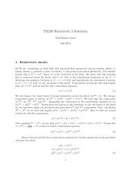
Figure 1 illustrates <strong>the</strong> dependence of <strong>the</strong> real parts of<br />
<strong>the</strong> roots, s 0 and s , on <strong>the</strong> wave number k <strong>for</strong> <strong>the</strong> case<br />
1 2 1 and 0 1 2 3. These roots<br />
have strictly negative real parts <strong>for</strong> all k, so <strong>the</strong> gauge<br />
source function H a is always driven toward <strong>the</strong> target<br />
gauge source function F a . At least <strong>for</strong> this simple case,<br />
H a approaches <strong>the</strong> target F a exponentially.<br />
Simple analytical expressions <strong>for</strong> <strong>the</strong> roots of <strong>the</strong> characteristic<br />
polynomial, Eq. (72), exist in <strong>the</strong> limits of small<br />
and large k. The large k limit is <strong>the</strong> most interesting,<br />
because it describes <strong>the</strong> sufficiently short wavelength perturbations<br />
of any spacetime. The asymptotic expressions<br />
<strong>for</strong> <strong>the</strong> large k roots are<br />
Re s 0 1<br />
1<br />
k<br />
Re s 2 1 2<br />
1<br />
2<br />
2<br />
1<br />
2<br />
O k 4 ; (73)<br />
1<br />
k<br />
2<br />
O k 4 :<br />
(74)<br />
These results show that <strong>the</strong> s modes are damped at<br />
approximately <strong>the</strong> rate 2 1 2 1=2 in <strong>the</strong> large k<br />
limit, while <strong>the</strong> damping rate <strong>for</strong> <strong>the</strong> s 0 mode approaches<br />
zero. These modes are stable <strong>for</strong> large enough k, <strong>the</strong>n, as<br />
2<br />
long as 1 1 > 0 and 2 1 2 1=2 > 0.<br />
B. Time-dependent F a<br />
Next we consider solutions to Eqs. (68) and (69) <strong>for</strong> <strong>the</strong><br />
case where F a is a specified function of time: F a<br />
F a t . In principle <strong>the</strong> <strong>equations</strong> could be solved analytically<br />
by Laplace trans<strong>for</strong>ming <strong>the</strong> <strong>equations</strong> in time, and<br />
solving <strong>for</strong> each frequency component of H a t separately.<br />
Instead it is more straight<strong>for</strong>ward, and perhaps<br />
more instructive, to integrate <strong>the</strong> <strong>equations</strong> numerically<br />
<strong>for</strong> some illustrative F a t . We assume <strong>for</strong> this simple<br />
example that <strong>the</strong> shift of <strong>the</strong> background spacetime van-<br />
0.0<br />
-0.5<br />
-1.0<br />
Re(s 0<br />
/µ)<br />
Re(s ±<br />
/µ)<br />
-1.5<br />
0 2 4 6 8 10<br />
k/µ<br />
FIG. 1 (color online). Real part of <strong>the</strong> characteristic frequencies<br />
of <strong>the</strong> gauge-driver system: s 0 and s .<br />
084001-9
LINDBLOM et al. PHYSICAL REVIEW D 77, 084001 (2008)<br />
ishes, 0, and <strong>the</strong> o<strong>the</strong>r parameters that determine <strong>the</strong><br />
system take <strong>the</strong> values 1 2 1 and 0 1<br />
2 3. We have solved <strong>the</strong> resulting simplified <strong>equations</strong><br />
numerically <strong>for</strong> <strong>the</strong> case F a t 3 e t 10 2 =9 with k<br />
1. Equations (68) and (69) require initial conditions <strong>for</strong><br />
H a , @ t H a , and a. We use H a 0 F a 0 ,<br />
@ t H a 0 0, and a 0 k 2 H a 0 . These initial<br />
data <strong>for</strong> H a and its time derivative were chosen to be<br />
fairly well matched with <strong>the</strong> target F a . They are similar to<br />
<strong>the</strong> initial conditions used in our more realistic tests in<br />
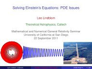
Sec. V. This target F a changes significantly <strong>for</strong> times near<br />
t 10, so this test explores how well <strong>the</strong> gauge-driver<br />
system is able to track an evolving target F a . Figure 2<br />
shows that <strong>the</strong> gauge-driver equation is fairly successful (at<br />
<strong>the</strong> few percent accuracy level) in driving H a t toward<br />
F a t <strong>for</strong> * 2 even in this ra<strong>the</strong>r dynamical situation.<br />
C. Coupled systems<br />
Finally we investigate <strong>the</strong> stability of <strong>the</strong> coupled gaugedriver<br />
and GH <strong>Einstein</strong> <strong>equations</strong> <strong>for</strong> perturbations of flat<br />
spacetime. The perturbed <strong>Einstein</strong> system reduces to a<br />
relatively simple <strong>for</strong>m 2 in this case:<br />
cd @ c @ d ab @ a H b @ b H a 0: (75)<br />
||δH - δF|| / ||δF||<br />
10 0 µ = 1/2<br />
µ = 1<br />
µ = 2<br />
µ = 4<br />
10 -1<br />
10 -2<br />
used to express H a and jl in terms of ^ta <strong>for</strong> <strong>the</strong> case<br />
^s 0:<br />
H^t<br />
^s 2 k 2<br />
2^s<br />
µ = 8<br />
10 -3<br />
0 5 10 15 20 25<br />
t<br />
FIG. 2 (color online). Response of <strong>the</strong> gauge-driver system to a<br />
time-dependent F a of <strong>the</strong> <strong>for</strong>m F a 3 e t 10 2 =9 , initial<br />
conditions H a 0 F a 0 , @ t H a 0 0, and a range of<br />
values <strong>for</strong> <strong>the</strong> damping parameter 1 2 1. This<br />
test uses k 1 and 1 2 3 0.<br />
^t ^t; (81)<br />
We study <strong>the</strong> stability of <strong>the</strong> coupled system, Eqs. (68),<br />
(69), and (75), by Laplace trans<strong>for</strong>ming <strong>the</strong> <strong>equations</strong> in<br />
time, i.e., by considering solutions with time dependence<br />
e st . In this case Eqs. (68) and (69) can be reduced to <strong>the</strong><br />
single equation,<br />
P s H a<br />
2<br />
1 1<br />
where P s is defined by<br />
1s<br />
s 1<br />
P s ^s 2 2 2 1 2 ^s k 2 2 1 1 1<br />
1<br />
s 1<br />
fk 2 2 1 1 2i k 2 1 3<br />
F a ; (76)<br />
^s 2 2 3 2 i k g: (77)<br />
We use <strong>the</strong> notation ^s s ik . The analogous expressions<br />
<strong>for</strong> <strong>the</strong> Laplace trans<strong>for</strong>m of <strong>the</strong> GH <strong>Einstein</strong> system,<br />
Eq. (75), are given by<br />
0 ^s 2 k 2 ^t ^t 2^s H^t ; (78)<br />
0 ^s 2 k 2 ^tj ^s H j ik j H^t ; (79)<br />
0 ^s 2 k 2 jl ik j H l ik l H j ; (80)<br />
where H^t H t N j H j , etc. These <strong>equations</strong> can be<br />
2 In this analysis we assume that <strong>the</strong> gauge constraint H a<br />
a 0 is satisfied. The analysis of <strong>the</strong> GH <strong>Einstein</strong> constraint<br />
evolution system in Ref. [4] shows that violations of this constraint<br />
are damped exponentially <strong>for</strong> perturbations of flat<br />
spacetime.<br />
H j<br />
^s 2 k 2<br />
^s 2 ^s ^tj<br />
1<br />
2 ik j ^t ^t ; (82)<br />
jl ^s 2 i^sk j ^tl i^sk l ^tj k j k l ^t ^t : (83)<br />
The case ^s 0 is essentially trivial: In this case k 2 ^t ^t<br />
0, k 2 ^tj ik j H^t , k 2 jl ik j H l ik l H j , and<br />
H a F a . The metric perturbation in this case is pure<br />
gauge (an infinitesimal coordinate trans<strong>for</strong>mation generated<br />
by <strong>the</strong> time-independent H a =k 2 ), and <strong>the</strong> gauge<br />
source function H a is identical to <strong>the</strong> target F a in this<br />
case. So we focus on <strong>the</strong> ^s 0 case <strong>for</strong> <strong>the</strong> remainder of<br />
this discussion.<br />
We consider in detail now <strong>the</strong> coupled gauge-driver<br />
system <strong>for</strong> <strong>the</strong> case of Bona-Massó slicing with 0,<br />
and <strong>the</strong> -driver shift condition. The perturbed flat-space<br />
limit of F a <strong>for</strong> <strong>the</strong> Bona-Massó driver, Eq. (53) with<br />
0, is given by<br />
F^t ^s f 1 1 i k 1<br />
^t ^t i 1 1 k l<br />
2f 1 2f 1<br />
^tl<br />
1<br />
1 1 ^s l l<br />
2<br />
; (84)<br />
while <strong>the</strong> target <strong>for</strong> <strong>the</strong> -driver shift condition, Eq. (63),<br />
reduces to<br />
F j ^s 2s ^tj i<br />
i<br />
2<br />
2s 1<br />
s 2<br />
2s<br />
s 2<br />
1 jl k l i<br />
2 k j ^t ^t<br />
1 k j l l : (85)<br />
084001-10
GAUGE DRIVERS FOR THE GENERALIZED HARMONIC ... PHYSICAL REVIEW D 77, 084001 (2008)<br />
The spatial metric perturbations, jl , that appear in<br />
Eqs. (84) and (85) can be replaced by ^ta using Eq. (83):<br />
F^t ^s f 1 1<br />
2f 1<br />
F j<br />
i<br />
2<br />
i k 1<br />
2f 1<br />
k 2 1 1<br />
2^s<br />
^t ^t; (86)<br />
k 2<br />
^s 2 2s 1 1 1 k<br />
s j ^t ^t<br />
2<br />
k 2 2s<br />
1<br />
^s s<br />
2s ^s ^tj<br />
2<br />
2s<br />
k<br />
^s s j k l ^tl : (87)<br />
2<br />
Now substitute <strong>the</strong>se expressions <strong>for</strong> F a , Eqs. (86) and<br />
(87), and <strong>the</strong> expressions <strong>for</strong> H a , Eqs. (81) and (82), into<br />
<strong>the</strong> perturbed gauge-driver Eq. (76). The result is a system<br />
of linear algebraic <strong>equations</strong> <strong>for</strong> ^ta . This system can be<br />
decoupled, and nontrivial solutions exist if and only if <strong>the</strong><br />
frequency s satisfies one of <strong>the</strong> following characteristic<br />
polynomials:<br />
0<br />
0<br />
^s 2 k 2<br />
2<br />
P s<br />
^s<br />
1 1<br />
^s 1 f 1<br />
f 1<br />
i k 1<br />
f 1<br />
^s 2 k 2<br />
2<br />
P s<br />
^s<br />
1 1<br />
k 2<br />
^s<br />
2s 1 s 2<br />
1s<br />
s 1<br />
1 1<br />
1s<br />
s 1<br />
k2^s<br />
; (88)<br />
1 2s ^s ; (89)<br />
The asymptotic <strong>for</strong>ms of <strong>the</strong> roots of <strong>the</strong> longitudinal<br />
modes (in which k j ^tj 0), Eq. (89), are given by<br />
Re s<br />
1<br />
4 f 1 2 2 1 2<br />
Re s 2 O k 2 ; (93)<br />
4 2 1 2 1 1 1 1 g 1=2<br />
1<br />
4 1 2 2 1 2 O k 2 : (94)<br />
Finally <strong>the</strong> asymptotic <strong>for</strong>ms of <strong>the</strong> roots of <strong>the</strong> transverse<br />
modes (in which k 2 g ij k i k j ^tj 0), Eq. (90), are<br />
given by<br />
2<br />
Re s 2 O k 2 ; (95)<br />
1<br />
Re s<br />
4 f 1 2 2 1<br />
2<br />
2<br />
4 2 1 2 1 1 1 g 1=2<br />
1<br />
4 1 2 2 1 2 O k 2 : (96)<br />
All four sign combinations represent distinct roots in<br />
Eqs. (92), (94), and (96). Stability of <strong>the</strong> gauge-driver<br />
system requires Re s < 0. There<strong>for</strong>e, stability of <strong>the</strong> short<br />
wavelength modes requires <strong>the</strong> following inequalities on<br />
<strong>the</strong> system parameters:<br />
0 < 1 1 ; (97)<br />
0 < 1 2 2 1 2 ; (98)<br />
0 < 1 1 1<br />
1 f 1<br />
f 1<br />
; (99)<br />
^s 2 k 2<br />
2<br />
k 2<br />
0 P s<br />
2s<br />
^s<br />
1 1<br />
^s s<br />
2s ^s ;<br />
2<br />
(90)<br />
where P s is defined in Eq. (77).<br />
The flat-space stability analysis presented here is relevant<br />
to generic spacetimes when <strong>the</strong> wave number k of <strong>the</strong><br />
perturbation becomes sufficiently large. We have solved<br />
<strong>the</strong> characteristic polynomials in Eqs. (88)–(90) in this<br />
limit. The leading order expressions <strong>for</strong> <strong>the</strong> real parts of<br />
<strong>the</strong>se roots are given as follows. For <strong>the</strong> time slicing modes<br />
(in which ^t ^t 0), <strong>the</strong> roots of Eq. (88), we have<br />
Re s<br />
Re s<br />
1<br />
4<br />
1<br />
2<br />
1 1<br />
1<br />
2 2 k 2 O k 4 ; (91)<br />
1 2 2 1 2<br />
4 2 1 1 1 1<br />
1<br />
4<br />
2<br />
1 f 1<br />
f 1<br />
1=2<br />
1 2 2 1 2 O k 2 : (92)<br />
0 < 2 ; (100)<br />
0 < 2 1 1 1 1 ; (101)<br />
0 < 2 1 1 1 : (102)<br />
We note that <strong>the</strong>se conditions can be satisfied <strong>for</strong> small<br />
values of by taking 1 > 0, 2 > 0, 2 > 0, 1 < 1,<br />
2 < 1, 1 > 0, 2 > 0, 0
LINDBLOM et al. PHYSICAL REVIEW D 77, 084001 (2008)<br />
0.2<br />
0<br />
max[Re(s)]<br />
-0.05<br />
-0.1<br />
-0.15<br />
-0.2<br />
µ = 1/4<br />
µ = 1/2<br />
µ = 1<br />
µ = 2<br />
µ = 4<br />
-0.25<br />
-0.2<br />
0 0.5 1 1.5<br />
0 0.2 0.4 0.6 0.8<br />
f(1)<br />
β<br />
1<br />
this case are 0, 1 2 1 32 2, 1 2 tems are solved numerically <strong>for</strong> <strong>the</strong>se cases. We measure<br />
1<br />
3 0, 1 2 2 , f 1 1<br />
2 , 3<br />
4 , and 1<br />
3 . <strong>the</strong> stability and effectiveness of <strong>the</strong> gauge-driver system in<br />
FIG. 3 (color online). Maximum damping rate of <strong>the</strong> modes as FIG. 5 (color online). Maximum damping rate of <strong>the</strong> modes as<br />
a function of <strong>the</strong> Bona-Massó slicing condition parameter f 1 . a function of <strong>the</strong> shift parameter . The o<strong>the</strong>r parameters used<br />
1<br />
The o<strong>the</strong>r parameters used <strong>for</strong> this case are k 1, 0, <strong>for</strong> this case are k 1, 1 2 1<br />
1<br />
1<br />
1 2 1 32 2, 1 2 3 0, 1 2 2 ,<br />
32 2, 1<br />
1<br />
2 3 0, 1 2<br />
3<br />
4 , and 1<br />
3 . 2 , f 1 1<br />
2 , 3<br />
4 , and 1<br />
3 .<br />
sponds to <strong>the</strong> length scale on which <strong>the</strong> gauge condition<br />
in our numerical tests of <strong>the</strong> gauge-driver system in Sec. V.<br />
needs to be en<strong>for</strong>ced most effectively.<br />
We also note that <strong>the</strong> standard value, f 1 2, used <strong>for</strong><br />
Figure 5 illustrates <strong>the</strong> dependence of max Re s on <strong>the</strong><br />
one-plus-log slicing by most of <strong>the</strong> numerical relativity<br />
background shift parameter <strong>for</strong> a range of values of <strong>the</strong><br />
community [8–11] is unstable when used in our gaugedriver<br />
<strong>equations</strong>. This does not imply that f 1 2 is a bad<br />
gauge-driver damping coefficients 1 2 1<br />
1<br />
choice when used in a standard three-plus-one evolution, 32 2. For small values of we see that <strong>the</strong> system is stable;<br />
only that it is unstable when used with our gauge-driver however, <strong>for</strong> > 1 2<br />
<strong>the</strong> system becomes unstable. This<br />
system.<br />
instability may be important in more realistic problems<br />
Figure 4 illustrates <strong>the</strong> k dependence of max Re s <strong>for</strong> a that involve black holes. Even <strong>for</strong> single black-hole spacetimes,<br />
<strong>the</strong> usual time-independent coordinate representa-<br />
range of values of <strong>the</strong> gauge-driver damping coefficients<br />
1<br />
1 2 1 32 2. For short wavelength perturbations,<br />
i.e., <strong>for</strong> values of k with k * , max Re s de-<br />
horizon. Binary black-hole spacetimes also use large shifts<br />
tions have nonvanishing shifts with 1 near <strong>the</strong><br />
creases as increases. Thus <strong>the</strong> solutions with large k are (with >1 in many cases) when coordinates that corotate<br />
damped more effectively as increases. However, <strong>for</strong> long with <strong>the</strong> black holes are used. We explore <strong>the</strong> stability of<br />
wavelength perturbations, i.e., <strong>for</strong> values of k with k & , this gauge-driver system <strong>for</strong> <strong>the</strong> case of single black-hole<br />
max Re s increases as increases. Thus <strong>the</strong> solutions spacetimes in Sec. V.<br />
with small k are less efficiently damped as increases. It We have also examined several o<strong>the</strong>r slicing and shift<br />
follows that <strong>the</strong>re is an optimal value of to use <strong>for</strong> any conditions using <strong>the</strong>se perturbation techniques. As a consequence<br />
of Sec. IVA, our gauge-driver system is stable <strong>for</strong><br />
particular problem: choose k c , where 1=k c corre-<br />
<strong>harmonic</strong> slicing F^t 0 and <strong>harmonic</strong> shift F i 0.We<br />
also find that <strong>the</strong> combinations of a stable Bona-Massó<br />
0<br />
-0.1<br />
-0.2<br />
slicing condition with <strong>harmonic</strong> shift, and of <strong>harmonic</strong><br />
µ = 1<br />
µ = 2<br />
en<strong>for</strong>ced through our gauge-driver <strong>equations</strong>.<br />
slicing with <strong>the</strong> -driver shift condition, are stable.<br />
µ = 1/4<br />
However, we find that <strong>the</strong> maximal slicing and<br />
µ = 1/2<br />
-freezing conditions are unconditionally unstable when<br />
µ = 4<br />
-0.3<br />
V. NUMERICAL TESTS<br />
-0.4<br />
In this section we describe <strong>the</strong> results of 3D numerical<br />
-0.5<br />
tests of <strong>the</strong> gauge-driver system. We consider two cases:<br />
0 2 4 6 8 10<br />
k<br />
first a Schwarzschild black hole with perturbed lapse and<br />
shift, and second a Schwarzschild black hole with a superimposed<br />
FIG. 4 (color online). Maximum damping rate of <strong>the</strong> modes as<br />
outgoing physical gravitational wave pulse. The<br />
a function of <strong>the</strong> wave number k. The o<strong>the</strong>r parameters used <strong>for</strong> full coupled nonlinear GH <strong>Einstein</strong> and gauge-driver sys-<br />
max[Re(s)]<br />
max[Re(s)]<br />
0.1<br />
0<br />
-0.1<br />
µ = 1/4<br />
µ = 1/2<br />
µ = 1<br />
µ = 2<br />
µ = 4<br />
084001-12
GAUGE DRIVERS FOR THE GENERALIZED HARMONIC ... PHYSICAL REVIEW D 77, 084001 (2008)<br />
<strong>the</strong>se tests as it attempts to drive <strong>the</strong> gauge toward Bonas<br />
2M C<br />
Massó slicing and -driver shift conditions.<br />
N 1<br />
These numerical tests are conducted using <strong>the</strong> infrastructure<br />
R R 4 ; (105)<br />
of <strong>the</strong> Caltech/Cornell Spectral <strong>Einstein</strong> Code<br />
(SpEC). This code uses pseudospectral collocation methods,<br />
as described, <strong>for</strong> example, in Refs. [13,14]. We use <strong>the</strong><br />
N i C^r i 2M C 2<br />
R 2 1<br />
R R 4 ; (106)<br />
<strong>generalized</strong> <strong>harmonic</strong> <strong>for</strong>m of <strong>the</strong> <strong>Einstein</strong> <strong>equations</strong>, as<br />
described in Ref. [4]. The evolution <strong>equations</strong> <strong>for</strong> <strong>the</strong> where ^r i is <strong>the</strong> outward directed radial unit vector:<br />
combined GH <strong>Einstein</strong> and <strong>the</strong> gauge-driver system are g ij ^r i ^r j 1.<br />
integrated in time using <strong>the</strong> adaptive fifth-order Cash-Karp We perturb this spacetime by changing <strong>the</strong> initial values<br />
method [15]. We use a <strong>for</strong>m of spectral filtering, as described<br />
in Ref. [13], that sets to zero in each time step <strong>the</strong> of perturbation changes <strong>the</strong> spacetime coordinates (or<br />
of <strong>the</strong> lapse and shift, and <strong>the</strong>ir time derivatives. This type<br />
changes in <strong>the</strong> top four tensor spherical <strong>harmonic</strong> expansion<br />
coefficients of each of our evolved quantities. This we perturb <strong>the</strong> lapse and shift of Eqs. (105) and (106) by<br />
gauge) of <strong>the</strong> solution, but not its geometry. For <strong>the</strong>se tests<br />
filtering step is needed to eliminate an instability associated<br />
adding<br />
with <strong>the</strong> inconsistent mixing of tensor spherical har-<br />
monics in our approach.<br />
Initial conditions are needed <strong>for</strong> any evolution of <strong>the</strong><br />
N A sin 2 r=r 0 e r r c 2 =w 2 Y lm ; (107)<br />
combined GH <strong>Einstein</strong> and gauge-driver systems, and<br />
N i A sin 2 r=r 0 e r r c 2 =w 2 Y lm ^r i ; (108)<br />
<strong>the</strong>se initial data consist of <strong>the</strong> spacetime metric ab , <strong>the</strong><br />
gauge source function H a , and <strong>the</strong>ir time derivatives. For where Y lm is <strong>the</strong> standard scalar spherical <strong>harmonic</strong>. In our<br />
<strong>the</strong> tests described here we take <strong>the</strong> initial spacetime metric numerical tests we use <strong>the</strong> background metric with C<br />
ab to be <strong>the</strong> Schwarzschild geometry plus perturbations as 1:73M 2 , and perturbations with A 0:01, r c 15M, w<br />
described in Secs. VA and V B. We set <strong>the</strong> time derivatives 3M, l 2, m 0, and various values of <strong>the</strong> radial wavelength<br />
r 0 .<br />
of <strong>the</strong> spatial components of <strong>the</strong> metric to zero <strong>for</strong> <strong>the</strong> pure<br />
gauge perturbation test in Sec. VA, and equal to <strong>the</strong> We per<strong>for</strong>m <strong>the</strong>se numerical tests on a computational<br />
appropriate time derivative of <strong>the</strong> superimposed physical domain consisting of a spherical shell that extends from<br />
gravitational wave pulse <strong>for</strong> <strong>the</strong> test in Sec. V B. The r 0:78M (just inside <strong>the</strong> horizon in <strong>the</strong>se coordinates) to<br />
remaining initial data needed <strong>for</strong> <strong>the</strong>se evolutions, @ t N, r 30M. We divide this domain into eight subdomains. In<br />
@ t N i , H a , and @ t H a , are pure gauge quantities. The time each subdomain we express each Cartesian component of<br />
derivatives of <strong>the</strong> lapse and shift are chosen here to ensure each dynamical field as a sum of Chebyshev polynomials<br />
that H a satisfies <strong>the</strong> desired gauge condition, H a F a , of r (through order N r 1) multiplied by scalar spherical<br />
initially. And finally <strong>the</strong> initial value of H a is chosen here <strong>harmonic</strong>s (through order L). The radii of <strong>the</strong> inner and<br />
to ensure that <strong>the</strong> gauge constraint, C a H a a 0, outer edges of <strong>the</strong> various subdomains are adjusted to<br />
vanishes initially.<br />
distribute <strong>the</strong> truncation error <strong>for</strong> this problem more or<br />
less uni<strong>for</strong>mly. The specific radii of <strong>the</strong> subdomain<br />
boundaries used in this test are 0:78M, 2:38M, 4:6M,<br />
8:83M, 13:07M, 17:30M, 21:53M, 25:77M, and 30:0M,<br />
respectively. The values of <strong>the</strong> parameters associated with<br />
<strong>the</strong> gauge-driver system used <strong>for</strong> this test are<br />
3<br />
A. Black hole with gauge perturbation<br />
For this test we consider a Schwarzschild black hole<br />
with perturbations in <strong>the</strong> lapse and shift. For <strong>the</strong> unperturbed<br />
hole we use isotropic spatial coordinates and maximal<br />
time slices [16,17]. The unperturbed spatial metric in<br />
this representation is given by<br />
ds 2 g ij dx i dx j R 2<br />
dx<br />
2<br />
dy 2 dz 2 ; (103)<br />
r<br />
where r 2 x 2 y 2 z 2 , and R r (<strong>the</strong> areal radius) satisfies<br />
<strong>the</strong> differential equation,<br />
dR<br />
dr<br />
R<br />
r<br />
s<br />
1<br />
2M<br />
R<br />
C 2<br />
R 4<br />
: (104)<br />
The constant M is <strong>the</strong> mass of <strong>the</strong> hole, and C is a<br />
parameter that specifies <strong>the</strong> particular maximal slicing.<br />
Finally, <strong>the</strong> unperturbed lapse N and shift N i <strong>for</strong> this<br />
representation of Schwarzschild are given by<br />
1<br />
0,<br />
3 , 1<br />
1 2 2 , 1 2 3 0, and various<br />
1<br />
values of <strong>the</strong> parameter 1 2 1 32 2. The<br />
Bona-Massó slicing condition used here has f N<br />
1=2N, and includes a target value <strong>for</strong> <strong>the</strong> extrinsic curvature<br />
K 0 ; <strong>for</strong> this test we set K 0 0.<br />
Figure 6 illustrates <strong>the</strong> constraint violations <strong>for</strong> a set of<br />
representative evolutions from this test, and demonstrates<br />
<strong>the</strong> exponential convergence of our numerical method. The<br />
solid curves represent <strong>the</strong> constraints associated with <strong>the</strong><br />
GH <strong>Einstein</strong> system, while <strong>the</strong> dotted curves represent <strong>the</strong><br />
constraints of <strong>the</strong> gauge-driver system. We measure <strong>the</strong><br />
constraint violations of <strong>the</strong> GH <strong>Einstein</strong> system <strong>for</strong> <strong>the</strong>se<br />
tests using <strong>the</strong> norm jjC GH jj defined in Eq. (71) of Ref. [4].<br />
The norm jjC GH jj is scaled so that it becomes of order unity<br />
when constraint violations start to dominante <strong>the</strong> solution.<br />
We define an analogous norm jjC H jj <strong>for</strong> <strong>the</strong> gauge-driver<br />
4 ,<br />
084001-13
LINDBLOM et al. PHYSICAL REVIEW D 77, 084001 (2008)<br />
10 -3<br />
10 -4<br />
N r<br />
= 9, L = 7<br />
10 -5<br />
10 -6<br />
10 -7<br />
10 -8<br />
N r<br />
= 13, L = 10<br />
N r<br />
= 17, L = 13<br />
10 -9<br />
0 100 200 300 400<br />
t/M<br />
FIG. 6 (color online). Solid curves show <strong>the</strong> constraints of <strong>the</strong><br />
GH <strong>Einstein</strong> system jjC GH jj, dotted curves show <strong>the</strong> constraints<br />
of <strong>the</strong> gauge-driver system jjC H jj <strong>for</strong> a test with 1:0=M and<br />
radial wavelength r 0 6:0M evolved at several numerical resolutions.<br />
||H - F|| / ||F||<br />
10 0 µ = 0.5/Μ<br />
10 -1<br />
µ = 1.0/Μ<br />
µ = 1.5/Μ<br />
10 -2<br />
µ = 2.0/Μ<br />
10 -3<br />
10 -4<br />
10 -5<br />
10 -6<br />
0 100 200 300 400<br />
t/M<br />
FIG. 7 (color online). Effectiveness of <strong>the</strong> gauge-driver equation<br />
is demonstrated by showing jjH Fjj=jjFjj <strong>for</strong> evolutions<br />
with radial wavelength r 0 6M and several values of <strong>the</strong> gauge<br />
damping parameter M 2f 1 2 ; 1; 3 2<br />
; 2g. These tests evolve a<br />
Schwarzschild black hole with strongly perturbed lapse and shift.<br />
system:<br />
Z<br />
jjC H jj 2 p gm<br />
ab g ij C H ia CH jb<br />
Z<br />
g kl C H ika CH jlb d3 x<br />
p gm<br />
cd g ij H H<br />
@ i H c @ j H d @ i c @ j d<br />
g kl @ i<br />
H<br />
kc<br />
@ j<br />
H<br />
ld<br />
d 3 x<br />
1<br />
: (109)<br />
The quantity m ab is a positive definite matrix, which we set<br />
to <strong>the</strong> identity matrix, m ab ab , <strong>for</strong> <strong>the</strong>se tests. Figure 6<br />
shows <strong>the</strong> constraints <strong>for</strong> a particular test run with<br />
1:0=M and r 0 6:0M. The analogous graphs <strong>for</strong> <strong>the</strong> o<strong>the</strong>r<br />
tests reported here are qualitatively similar, with somewhat<br />
larger but still convergent ‘‘spikes’’ in jjC GH jj at early<br />
times (t & 25M) <strong>for</strong> <strong>the</strong> 0:5=M case. Figure 6 shows<br />
that <strong>the</strong> constraints are well satisfied in our evolutions, and<br />
demonstrates that our numerical methods are (exponentially)<br />
convergent. The growth in <strong>the</strong> constraints seen at<br />
late times is a mild power law, approximately t 3=4 , and is<br />
not something that concerns us.<br />
Figure 7 illustrates <strong>the</strong> effectiveness of <strong>the</strong> gauge-driver<br />
system, at least <strong>for</strong> this test problem. We measure <strong>the</strong><br />
difference between <strong>the</strong> gauge source function H a and <strong>the</strong><br />
target function to which it is being driven, F a , using <strong>the</strong><br />
following L 2 norm:<br />
R<br />
jjH Fjj 2 p gm<br />
ab H a F a H b F b d 3 x<br />
R<br />
jjFjj 2 p gm<br />
cd F c F d d 3 ; (110)<br />
x<br />
where (as be<strong>for</strong>e) <strong>the</strong> matrix m ab is set to <strong>the</strong> identity,<br />
m ab ab , <strong>for</strong> <strong>the</strong>se tests. This norm is scaled so that<br />
H a bears little resemblance to <strong>the</strong> target F a whenever <strong>the</strong><br />
norm becomes of order unity. Figure 7 shows that <strong>the</strong><br />
gauge perturbation used in this test violates <strong>the</strong> desired<br />
gauge conditions ra<strong>the</strong>r severely at early times. The norm<br />
jjH Fjj=jjFjj is driven to values as large as 0.7 at about<br />
t 20M when <strong>the</strong> ingoing part of <strong>the</strong> gauge perturbation<br />
interacts most strongly with <strong>the</strong> black hole. After this<br />
initial interaction, <strong>the</strong> gauge-driver system takes over and<br />
effectively drives jjH Fjj=jjFjj to values below 10 3 on<br />
time scales of 40M to 60M, depending on <strong>the</strong> value of <strong>the</strong><br />
gauge damping parameter used in <strong>the</strong> evolution. Figure 7<br />
shows evolutions of gauge perturbations with radial wavelength<br />
r 0 6M, and several values of <strong>the</strong> damping parameter<br />
M 2f 1 2 ; 1; 3 2<br />
; 2g computed with numerical<br />
resolution N r 17 and L 13. The gauge-driver system<br />
is more effective at reducing jjH Fjj=jjFjj quickly at<br />
early times, t
GAUGE DRIVERS FOR THE GENERALIZED HARMONIC ... PHYSICAL REVIEW D 77, 084001 (2008)<br />
||H - F|| / ||F||<br />
10 0 r 0<br />
= 4 M<br />
10 -1<br />
10 -2<br />
10 -3<br />
10 -4<br />
10 -5<br />
r 0<br />
= 6 M<br />
r 0<br />
= 8 M<br />
r 0<br />
= 10 M<br />
10 -6<br />
0 100 200 300 400<br />
t/M<br />
FIG. 8 (color online). Effectiveness of <strong>the</strong> gauge-driver equation<br />
is demonstrated by showing jjH Fjj=jjFjj <strong>for</strong> evolutions<br />
with 0:5=M and several values of <strong>the</strong> radial wavelength of<br />
<strong>the</strong> perturbation r 0 2f4M; 6M; 8M; 10Mg. These tests evolve a<br />
Schwarzschild black hole with strongly perturbed lapse and shift.<br />
||H - F|| / ||F||<br />
10 -3<br />
10 -4<br />
N r<br />
= 21, L = 8<br />
N r<br />
= 31, L = 10<br />
10 -5<br />
10 -6<br />
N r<br />
= 41, L = 12<br />
N r<br />
= 51, L = 14<br />
10 -7<br />
0 100 200 300 400<br />
t/M<br />
FIG. 9 (color online). Effectiveness of <strong>the</strong> gauge-driver equation<br />
is demonstrated by showing jjH Fjj=jjFjj <strong>for</strong> evolutions<br />
with 0:25=M obtained with a variety of numerical resolutions.<br />
This test uses a Schwarzschild black hole with a superimposed<br />
outgoing gravitational wave pulse.<br />
more quickly (at least at early times) <strong>for</strong> shorter wavelength<br />
perturbations. Our hope is that this ability to efficiently<br />
control short wavelength features of <strong>the</strong> gauge is<br />
what will be needed to prevent <strong>the</strong> kinds of localized gauge<br />
singularities that often appear in our evolutions of binary<br />
black-hole spacetimes.<br />
B. Black hole with physical perturbation<br />
Our second numerical test of <strong>the</strong> gauge-driver system<br />
uses a Schwarzschild black hole with a superimposed outgoing<br />
gravitational wave pulse, as described in<br />
Refs. [13,18]. The background solution is a Schwarzschild<br />
black hole in Kerr-Schild coordinates,<br />
ds 2 dt 2 2M<br />
dt dr 2 dx 2 dy 2 dz 2 ; (111)<br />
r<br />
where r 2 x 2 y 2 z 2 and M is <strong>the</strong> mass. We superimpose<br />
an odd-parity outgoing quadrupolar gravitational<br />
wave perturbation constructed using Teukolsky’s method<br />
[19]. Its generating function is taken to be a Gaussian,<br />
G r A exp r r 2 c =w 2 , with A 4 10 3 , r c<br />
5M, and w 1:5M. Using this perturbed Schwarzschild<br />
solution as <strong>the</strong> input con<strong>for</strong>mal metric, <strong>the</strong> full nonlinear<br />
initial value <strong>equations</strong> (in <strong>the</strong> con<strong>for</strong>mal thin sandwich<br />
<strong>for</strong>mulation) are solved to obtain initial data that satisfy<br />
<strong>the</strong> constraints [20]. This procedure yields initial values <strong>for</strong><br />
<strong>the</strong> spatial metric, extrinsic curvature, lapse, and shift. We<br />
note that <strong>the</strong> resulting solution to <strong>the</strong> constraints is still<br />
nearly (but not completely) outgoing.<br />
The computational domain <strong>for</strong> this test problem is taken<br />
to be a spherical shell extending from r 1:9M (just<br />
inside <strong>the</strong> horizon in <strong>the</strong>se coordinates) out to r<br />
41:9M. This domain is subdivided into four spherical-shell<br />
subdomains of width r 10M. On each subdomain, <strong>the</strong><br />
numerical solution is expanded in Chebyshev polynomials<br />
and spherical <strong>harmonic</strong>s as be<strong>for</strong>e. For <strong>the</strong>se tests we use<br />
numerical resolutions with N r 2f21; 31; 41; 51g coefficients<br />
per subdomain <strong>for</strong> <strong>the</strong> Chebyshev series and l L<br />
with L 2f8; 10; 12; 14g <strong>for</strong> <strong>the</strong> spherical <strong>harmonic</strong>s. The<br />
values of <strong>the</strong> parameters associated with <strong>the</strong> gauge-driver<br />
3<br />
system used <strong>for</strong> this test are<br />
4 , 0, 1<br />
3 , 1<br />
1<br />
2 2 , 1 2 3 0, and various values of <strong>the</strong> parameter<br />
1 2 1 32 2. The Bona-Massó<br />
1<br />
slicing condition used here has f N 1=2N, and includes<br />
a target value <strong>for</strong> <strong>the</strong> extrinsic curvature K 0 that is set equal<br />
to its value in <strong>the</strong> perturbed initial data.<br />
Figure 9 illustrates <strong>the</strong> effectiveness of <strong>the</strong> gauge-driver<br />
equation <strong>for</strong> imposing <strong>the</strong> Bona-Massó slicing and<br />
-driver shift conditions in evolutions of a Schwarzschild<br />
black hole with physical gravitational wave perturbation.<br />
These tests were per<strong>for</strong>med with <strong>the</strong> gauge damping parameter<br />
0:25=M. For this test we set <strong>the</strong> target value<br />
<strong>for</strong> <strong>the</strong> extrinsic curvature K 0 to that of an unperturbed<br />
Kerr-Schild spacetime. The various curves in Fig. 9 illustrate<br />
how jjH Fjj=jjFjj changes <strong>for</strong> evolutions per<strong>for</strong>med<br />
with different numerical resolutions. The results<br />
are qualitatively similar to those of <strong>the</strong> first test: <strong>the</strong> black<br />
hole with physical gravitational wave perturbation does not<br />
satisfy <strong>the</strong> target gauge conditions exactly at early times,<br />
but <strong>the</strong> gauge-driver equation reduces jjH Fjj=jjFjj to<br />
very small values by about t 75M. This test is less severe<br />
in some sense than our first pure gauge perturbation test,<br />
since <strong>the</strong> initial data in this case contains an outgoing<br />
gravitational wave pulse that never interacts very strongly<br />
with <strong>the</strong> black hole.<br />
VI. DISCUSSION<br />
We have presented a new gauge-driver evolution system<br />
in Sec. II that makes it possible to impose a wide range of<br />
gauge conditions in <strong>the</strong> GH <strong>for</strong>mulation of <strong>the</strong> <strong>Einstein</strong><br />
<strong>equations</strong>, without destroying its hyperbolicity. The key<br />
idea is to construct an auxiliary hyperbolic evolution equation<br />
<strong>for</strong> <strong>the</strong> gauge source function H a that drives it toward<br />
084001-15
LINDBLOM et al. PHYSICAL REVIEW D 77, 084001 (2008)<br />
<strong>the</strong> desired target F a . Section III shows how many of <strong>the</strong><br />
gauge conditions widely used by <strong>the</strong> numerical relativity<br />
community can be included in this way. In Sec. IV we<br />
analyze <strong>the</strong> effectiveness and stability of <strong>the</strong> combined GH<br />
<strong>Einstein</strong> and gauge-driver system <strong>for</strong> <strong>the</strong> case of perturbations<br />
of flat spacetime. This analysis shows that <strong>the</strong> gaugedriver<br />
equation effectively drives H a toward F a , when F a<br />
is specified a priori as a function of <strong>the</strong> spacetime coordinates.<br />
We were somewhat surprised to find, however, that<br />
<strong>the</strong> gauge-driver system can be quite unstable when it is<br />
coupled to <strong>the</strong> GH <strong>Einstein</strong> system. We found that common<br />
gauge conditions like maximal slicing and <strong>the</strong> -freezing<br />
gauge conditions are unconditionally unstable when implemented<br />
using our gauge-driver equation. This does not<br />
imply of course that those conditions are unsuitable <strong>for</strong> use<br />
with o<strong>the</strong>r <strong>for</strong>ms of <strong>the</strong> <strong>Einstein</strong> system (like <strong>the</strong><br />
Baumgarte-Shapiro-Shibata-Nakamura, BSSN, <strong>for</strong>mulation<br />
[12]), just that <strong>the</strong>y cannot be implemented in a<br />
completely stable way in <strong>the</strong> GH <strong>Einstein</strong> system coupled<br />
to <strong>the</strong> particular gauge-driver <strong>equations</strong> introduced here.<br />
Fortunately, we were able to find some of <strong>the</strong> commonly<br />
used gauge conditions that can be implemented in this way:<br />
certain Bona-Massó slicing conditions and a commonly<br />
used <strong>for</strong>m of <strong>the</strong> -driver shift conditions. Our 3D numerical<br />
tests in Sec. V show that <strong>the</strong> gauge-driver system can<br />
impose <strong>the</strong>se gauge conditions stably and effectively <strong>for</strong><br />
<strong>the</strong> evolutions of perturbed single black-hole spacetimes.<br />
There has been a great deal of discussion in <strong>the</strong> literature<br />
about <strong>the</strong> <strong>for</strong>mation of shocks when certain dynamical<br />
gauge conditions are imposed [21–23]. However, <strong>the</strong>se<br />
discussions do not apply when those same gauge conditions<br />
are imposed using a driver condition. The gaugedriver<br />
system imposes <strong>the</strong> desired gauge condition only<br />
approximately, not exactly. At best, <strong>the</strong> desired gauge<br />
condition is imposed exactly only asymptotically in time<br />
as <strong>the</strong> system approaches a time-independent equilibrium<br />
state, and even in this state shocks do not necessarily <strong>for</strong>m.<br />
On <strong>the</strong> contrary, <strong>the</strong>re are many solutions even to bad<br />
gauge conditions that do not have shocks. What determines<br />
whe<strong>the</strong>r an evolution system develops shocks is <strong>the</strong> structure<br />
of <strong>the</strong> operator that evolves <strong>the</strong> spacetime metric and<br />
auxiliary fields. Our evolution system (including <strong>the</strong><br />
gauge-driver system) has been carefully designed to be<br />
linearly degenerate, a condition that prevents <strong>the</strong> <strong>for</strong>mation<br />
of shocks (resulting from a crossing of characteristics)<br />
from smooth initial data [24]. Linear degeneracy does<br />
not prevent <strong>the</strong> <strong>for</strong>mation of curvature singularities, of<br />
course, or even <strong>the</strong> <strong>for</strong>mation of coordinate singularities<br />
that may arise from nonlinearities in <strong>the</strong> nonprincipal parts<br />
of <strong>the</strong> evolution <strong>equations</strong>.<br />
Causality is ano<strong>the</strong>r issue that appears to be less restrictive<br />
<strong>for</strong> our gauge-driver system than it is <strong>for</strong> directly<br />
imposed gauge conditions. For example, <strong>the</strong> parameter<br />
that appears in <strong>the</strong> -driver system discussed in Sec. III B<br />
3<br />
must take values in <strong>the</strong> range 0<br />
4<br />
in order <strong>for</strong> that<br />
driver to evolve <strong>the</strong> shift in a causal way in <strong>the</strong> BSSN<br />
system [25]. There is no such restriction on , however,<br />
when this driver is imposed through our gauge-driver<br />
system. In our system <strong>the</strong> shift is evolved, along with <strong>the</strong><br />
rest of <strong>the</strong> spacetime metric, by <strong>the</strong> GH <strong>Einstein</strong> system.<br />
This system is manifestly hyperbolic, and all of <strong>the</strong> fields<br />
propagate within <strong>the</strong> physical light cone, no matter what<br />
target gauge source function is used in <strong>the</strong> gauge-driver<br />
system.<br />
It is easy to imagine that <strong>the</strong> system presented here could<br />
be improved in several ways. It may be possible, <strong>for</strong><br />
example, to improve <strong>the</strong> per<strong>for</strong>mance of <strong>the</strong> system by<br />
<strong>for</strong>mulating boundary conditions <strong>for</strong> H a that impose <strong>the</strong><br />
desired gauge condition H a F a exactly at <strong>the</strong> boundaries.<br />
It may also be possible to <strong>for</strong>mulate a different evolution<br />
operator <strong>for</strong> H a that drives it more stably and/or<br />
more efficiently toward <strong>the</strong> desired target F a . Finally it<br />
may be possible to find better target gauge conditions F a .<br />
The ones studied here are those which have been found<br />
useful in evolutions of traditional three-plus-one <strong>for</strong>mulations<br />
of <strong>the</strong> <strong>Einstein</strong> system like BSSN. But <strong>the</strong>re may exist<br />
gauge conditions having much better stability and effectiveness<br />
properties when used as target gauge conditions<br />
within a gauge-driver system. These questions, and o<strong>the</strong>rs,<br />
will be addressed in future work on this problem.<br />
ACKNOWLEDGMENTS<br />
We thank Harald Pfeiffer and Bela Szilagyi <strong>for</strong> helpful<br />
comments concerning this work. The numerical simulations<br />
presented here were per<strong>for</strong>med using <strong>the</strong> Spectral<br />
<strong>Einstein</strong> Code (SpEC) developed at Caltech and Cornell<br />
primarily by Larry Kidder, Harald Pfeiffer, and Mark<br />
Scheel. This work was supported in part by grants from<br />
<strong>the</strong> Sherman Fairchild Foundation and <strong>the</strong> Brinson<br />
Foundation, by NSF Grant Nos. DMS-0553302, PHY-<br />
0601459, PHY-0652995, and by NASA Grant<br />
No. NNG05GG52G.<br />
[1] F. Pretorius, Classical Quantum Gravity 22, 425 (2005).<br />
[2] F. Pretorius, Phys. Rev. Lett. 95, 121101 (2005).<br />
[3] F. Pretorius, Classical Quantum Gravity 23, S529 (2006).<br />
[4] L. Lindblom, M. A. Scheel, L. E. Kidder, R. Owen, and O.<br />
Rinne, Classical Quantum Gravity 23, S447 (2006).<br />
[5] M. Holst, L. Lindblom, R. Owen, H. P. Pfeiffer, M. A.<br />
Scheel, and L. E. Kidder, Phys. Rev. D 70, 084017 (2004).<br />
[6] L. Smarr and J. W. York, Phys. Rev. D 17, 2529 (1978).<br />
084001-16
GAUGE DRIVERS FOR THE GENERALIZED HARMONIC ... PHYSICAL REVIEW D 77, 084001 (2008)<br />
[7] C. Bona, J. Massó, E. Seidel, and J. Stela, Phys. Rev. Lett.<br />
75, 600 (1995).<br />
[8] J. Balakrishna, G. Daues, E. Seidel, W.-M. Suen, M.<br />
Tobias, and E. Wang, Classical Quantum Gravity 13,<br />
L135 (1996).<br />
[9] M. Alcubierre, B. Brügmann, P. Diener, M. Koppitz, D.<br />
Pollney, E. Seidel, and R. Takahashi, Phys. Rev. D 67,<br />
084023 (2003).<br />
[10] M. Campanelli, C. O. Lousto, P. Marronetti, and Y.<br />
Zlochower, Phys. Rev. Lett. 96, 111101 (2006).<br />
[11] J. G. Baker, J. Centrella, D.-I. Choi, M. Koppitz, and J. van<br />
Meter, Phys. Rev. Lett. 96, 111102 (2006).<br />
[12] T. W. Baumgarte and S. L. Shapiro, Phys. Rev. D 59,<br />
024007 (1998).<br />
[13] L. E. Kidder, L. Lindblom, M. A. Scheel, L. T. Buchman,<br />
and H. P. Pfeiffer, Phys. Rev. D 71, 064020 (2005).<br />
[14] M. Boyle, L. Lindblom, H. P. Pfeiffer, M. A. Scheel, and<br />
L. E. Kidder, Phys. Rev. D 75,024006 (2007).<br />
[15] J. R. Cash and A. H. Karp, ACM Trans. Math. Softw. 16,<br />
201 (1990).<br />
[16] F. Estabrook, H. Wahlquist, S. Christensen, B. DeWitt, L.<br />
Smarr, and E. Tsiang, Phys. Rev. D 7, 2814 (1973).<br />
[17] G. B. Cook and H. P. Pfeiffer, Phys. Rev. D 70, 104016<br />
(2004).<br />
[18] O. Rinne, L. Lindblom, and M. A. Scheel, Classical<br />
Quantum Gravity 24, 4053 (2007).<br />
[19] S. A. Teukolsky, Phys. Rev. D 26, 745 (1982).<br />
[20] H. P. Pfeiffer, L. E. Kidder, M. A. Scheel, and D.<br />
Shoemaker, Phys. Rev. D 71, 024020 (2005).<br />
[21] M. Alcubierre, Phys. Rev. D 55, 5981 (1997).<br />
[22] M. Alcubierre and J. Massó, Phys. Rev. D 57, R4511<br />
(1998).<br />
[23] M. Alcubierre, Classical Quantum Gravity 22, 4071<br />
(2005).<br />
[24] T. P. Liu, J. Diff. Equ. 33, 92 (1979).<br />
[25] M. Alcubierre, B. Brügmann, P. Diener, M. Koppitz, D.<br />
Pollney, E. Seidel, and R. Takahashi, Phys. Rev. D 67,<br />
084023 (2003).<br />
084001-17