HYPROP manual - UMS
HYPROP manual - UMS
HYPROP manual - UMS

Create successful ePaper yourself
Turn your PDF publications into a flip-book with our unique Google optimized e-Paper software.
User Manual<br />
<strong>HYPROP</strong>
<strong>HYPROP</strong> system<br />
Table of content<br />
1 <strong>HYPROP</strong> system 5<br />
1.1 Safety instructions and warnings 5<br />
1.2 Content of delivery 6<br />
1.3 Expression of thanks 8<br />
1.4 Intended use 9<br />
1.5 Guarantee 10<br />
1.6 Important note 11<br />
2 Process summary 12<br />
3 Product description 13<br />
3.1 System components 13<br />
3.2 Sensor unit 13<br />
3.2.1 Main body 13<br />
3.2.2 Pressure transducers 14<br />
3.2.3 Tensiometers 15<br />
3.2.4 Temperature sensor 16<br />
3.2.5 Plug connector 16<br />
3.3 Sampling ring 16<br />
3.4 Software tensioVIEW ® 16<br />
4 Get ready to start a measuring campaign 18<br />
4.1 Soil samples 19<br />
4.1.1 Soil Sampling 19<br />
4.1.2 Saturate the samples 19<br />
4.2 Filling 21<br />
Important cautions 21<br />
4.2.1 Refilling of the <strong>HYPROP</strong> 24<br />
4.2.2 Degas ceramic tip and refill <strong>HYPROP</strong> shaft 24<br />
4.2.3 Degas the sensor head 27<br />
4.2.4 Reassemble the sensor unit 30<br />
4.2.5 Check the <strong>HYPROP</strong> 32<br />
4.3 Attach the sampling ring 33<br />
5 Set-up the <strong>HYPROP</strong> 35<br />
5.1 Connect the system components 35<br />
5.1.1 Scale 38<br />
5.2 Software tensioVIEW ® 41<br />
5.2.1 Menu 41<br />
5.2.1.1 Find devices 41<br />
5.2.1.2 Single device mode 41<br />
5.2.1.3 Multiplexed devices mode 41<br />
5.2.2 Device window 42<br />
5.2.2.1 Properties 42<br />
5.2.2.2 Configuration of a device 42<br />
5.2.2.3 Configuration settings for <strong>HYPROP</strong> 44<br />
5.2.3 Refilling window 46<br />
5.2.4 Current readings 47<br />
2/104
<strong>HYPROP</strong> system<br />
5.2.5 Stored readings 47<br />
5.3 Add the scale 48<br />
6 Perform a measuring campaign 50<br />
6.1 Starting conditions 50<br />
6.2 Measuring campaign window 52<br />
6.3 Configure the campaign 53<br />
6.4 Perform the measurement 54<br />
6.4.1 Single unit mode and multiplex device mode 54<br />
6.4.2 Start of a measuring campaign 54<br />
6.4.3 Constant starting conditions 54<br />
6.4.4 Start a spontaneou measurement 55<br />
6.4.5 Current status of the measurement 55<br />
6.4.6 Measurements in the „Single device mode“ 56<br />
6.4.7 Multiplex devices mode 57<br />
6.4.8 Interrupt a measuring campaign 58<br />
6.5 Description of an ideal measured curve 59<br />
6.6 Conclusion of a measurement 60<br />
6.7 Remove the soil sample 62<br />
6.8 Dry weight 65<br />
7 Evaluation 66<br />
8 Trouble shooting 67<br />
9 Service and maintenance 69<br />
9.1 Check the <strong>HYPROP</strong> 69<br />
9.1.1 Check the Zero point 69<br />
9.1.2 Check the Response 69<br />
9.1.3 Calibration 70<br />
9.1.4 Check the Offset 70<br />
9.2 Cleaning 70<br />
9.3 Storage 70<br />
9.4 Change the O-ring on the <strong>HYPROP</strong> sensor unit 71<br />
10 Theoretical basics 73<br />
10.1 Evaporation method (overview) 73<br />
10.2 Discrete data for retention and conductivity relation 73<br />
10.3 Retention and conductivity functions 74<br />
10.3.1 The van Genuchten/Mualem modell 75<br />
10.3.2 The bimodal van Genuchten/Mualem Model 75<br />
10.3.3 The Brooks and Corey Model 76<br />
10.4 Optimization of the parameter 76<br />
11 Additional notes 77<br />
11.1 Extended measuring range 77<br />
11.1.1 The bubble point of the porous cup 77<br />
11.1.2 The vapour pressure of water 77<br />
11.1.3 Boiling retardation: 78<br />
11.2 Vapour pressure influence on pF/WC 79<br />
3/104
<strong>HYPROP</strong> system<br />
11.3 Osmotic effect 79<br />
12 Appendix 80<br />
12.1 Typical measurement curves 80<br />
12.1.1 Sandy loam (Ls3) 80<br />
12.1.2 Clayey silt (Ut3) 83<br />
12.1.3 Slightly loamy Sand (Sl2) 85<br />
12.1.4 Reiner Fein- bis Mittelsand (Ss) 88<br />
12.2 Typical results for different soil 90<br />
12.3 Parameter list 91<br />
12.3.1 Input 91<br />
12.3.2 Output 92<br />
12.3.3 Parameter listing and describtion of the .csv table: 93<br />
12.4 Units for soil water and matric potentials 94<br />
12.5 Technical specifications 95<br />
12.5.1 Wiring configuration 96<br />
12.6 Accessories 97<br />
12.6.1 <strong>HYPROP</strong> extension and Accessories 97<br />
13 List of literature 99<br />
14 Index 102<br />
Your addressee at <strong>UMS</strong> 104<br />
4/104
<strong>HYPROP</strong> system<br />
1 <strong>HYPROP</strong> system<br />
Laboratory evaporation method according to WIND/SCHINDLER for<br />
the determination of unsaturated hydraulic conductivity and water<br />
retention characteristics of soil samples.<br />
1.1 Safety instructions and warnings<br />
Electrical installations must comply with the safety and EMC<br />
requirements of the country in which the system is to be used.<br />
Please note that any damages caused by users are not covered by<br />
warranty.<br />
Tensiometers are instruments for measuring the soil water tension,<br />
soil water pressure and soil temperature and are designed for this<br />
purpose only.<br />
Please be aware of the following warnings:<br />
High pressure: The maximum non destructive pressure is<br />
300 kPa = 3 bar = 3000 hPa. Higher pressure, which might occur<br />
for example during insertion in wet clayey soils or during refilling<br />
and reassembling, will damage the pressure transducer!<br />
Ceramic cup: Do not touch the cup with your fingers. Grease,<br />
sweat or soap residues will influence the ceramic's hydrophilic<br />
performance.<br />
Freezing: Tensiometers are filled with water and therefore are<br />
sensitive to freezing! Protect Tensiometers from freezing at any<br />
time. Never leave Tensiometers over night inside a cabin or car<br />
when freezing temperatures might occur!<br />
Do not use a sharp tool for cleaning the threads in the sensor unit.<br />
Just rinse it with pure water from a spray bottle.<br />
5/104
<strong>HYPROP</strong> system<br />
1.2 Content of delivery<br />
The delivery includes two bags and the package incl EG2200 Scale:<br />
Bag 1: (black lock, similar for each <strong>HYPROP</strong>-E) is consisting of<br />
(Figure 1-1) :<br />
• Sensor unit, set of Tensiometer shafts, 2 each 50 / 25 mm<br />
• acrylic attachment for sensor unit (3) Perforated saturation bowl<br />
(4)<br />
• <strong>HYPROP</strong> connecting cable (5), 6 pcs. filter fabric, 15 cm x 15<br />
cm (6), Silicone gasket (6)<br />
• tensioLINK ® T-piece junction plug(7) and silicone prot. caps (8)<br />
1<br />
3<br />
2<br />
8<br />
7<br />
5<br />
4<br />
6<br />
Figure 1-1<br />
6/104
<strong>HYPROP</strong> system<br />
Bag 2 (white lock): service kit, which includes (Figure 1-2):<br />
• Bottle of deionised water (1)<br />
• Syringes incl: 2 reservoir syringes (2), - 2 vacuum syringes (with<br />
red O-ring at tip) (3) 1 vacuum syringe with acrylic attachment (4)<br />
incl. tube (12) and 1 droplet syringe (5)<br />
• Sampling ring with 2 plastic caps* (6)<br />
• Tensiometer auger (7) and auger adapter (11)<br />
• Cable set consisting of: Mains power device* (9), <strong>HYPROP</strong><br />
USB- converter (10)<br />
• tensioVIEW ® software on CD<br />
5 4 3<br />
2<br />
7<br />
12<br />
11<br />
10<br />
8<br />
6<br />
1 9<br />
Figure 1-2<br />
7/104
<strong>HYPROP</strong> system<br />
1.3 Expression of thanks<br />
Dr. Uwe Schindler was able to considerably simplify the evaporation<br />
method by WIND by analyzing the evaporation process and the<br />
spatiotemporal decrease of water content inside the sample during<br />
the evaporation process. The results of surveys of more than 2000<br />
samples became part of German and international soil data bases<br />
(HYPRES, UNSODA) and were basis of many scientific studies.<br />
List of referring publications:<br />
1. Schindler, U. (1980): Ein Schnellverfahren zur Messung der<br />
Wasserleitfähigkeit im teilgesättigten Boden an<br />
Stechzylinderproben. Arch. Acker- u. Pflanzenbau u. Bodenkd.,<br />
Berlin 24, 1, 1-7.<br />
2. Schindler, U.; Bohne, K. and R. Sauerbrey (1985): Comparison<br />
of different measuring and calculating methods to quantify the<br />
hydraulic conductivity of unsaturated soil. Z. Pflanzenernähr.<br />
Bodenkd., 148, 607-617.<br />
3. Schindler U., Thiere, J., Steidl, J. und L. Müller (2004):<br />
Bodenhydrologische Kennwerte heterogener Flächeneinheiten-<br />
Methodik der Ableitung und Anwendungsbeispiel für<br />
Nordostdeutschland. Fachbeitrag des Landesumweltamtes.<br />
H.87. Bodenschutz 2. Landesumweltamt Brandenburg.<br />
Potsdam. 55 S.<br />
http://www.brandenburg.de/cms/media.php/2320/lua_bd87.pdf<br />
4. Schindler, U., Müller L. 2006. Simplifying the evaporation<br />
method for quantifying soil hydraulic properties. J. of Plant<br />
Nutrition and Soil Science. 169 (5). 169.623-629.<br />
Mr. Andre Peters, in his dissertation at the Institute for Geoecology of<br />
the Technical University Braunschweig, headed by Prof. Dr.<br />
Wolfgang Durner, has scientifically examined the theoretical<br />
principles of the calculation method and improved the method to be<br />
more precise. Furthermore, he developed the software SHYPFIT 2.0<br />
to adapt the retention and conductivity functions to the measured<br />
data, and implemented it in the <strong>HYPROP</strong> calculation software.<br />
The thesis is documented in following publications:<br />
1. Peters, A., and W. Durner (2008): Simplified Evaporation Method<br />
for Determining Soil Hydraulic Properties. Journal of Hydrology,<br />
under review.<br />
8/104
<strong>HYPROP</strong> system<br />
2. Peters, A., and W. Durner (2007): Optimierung eines einfachen<br />
Verdunstungsverfahrens zur Bestimmung bodenhydraulischer<br />
Eigenschaften, Mitteilungen der Deutschen Bodenkundlichen<br />
Gesellschaft, im Druck.<br />
3. Peters, A., and W. Durner (2006a): Improved estimation of soil<br />
water retention characteristics from hydrostatic column<br />
experiments, Water Resource. Res., 42, W11401,<br />
doi:10.1029/2006WR004952.<br />
4. Peters, A. und W. Durner (2006b), SHYPFIT 2.0 Users Manual,<br />
Internal Report. Institut für Geoökologie, Technische Universität<br />
Braunschweig.<br />
5. Peters, A., and W. Durner (2005): Verbesserte Methode zur<br />
Bestimmung der Retentionsfunktion aus statischen<br />
Säulenexperimenten, Mitteilungen der Deutschen<br />
Bodenkundlichen Gesellschaft. 107, 83-84.<br />
6. Peters, A., and W. Durner (2007): Optimierung eines einfachen<br />
Verdunstungsverfahrens zur Bestimmung bodenhydraulischer<br />
Eigenschaften, Tagung der Deutschen Bodenkundlichen<br />
Gesellschaft, Dresden, 2-.9.September 2007. URL:<br />
http://www.soil.tu-bs.de/pubs/poster/2007.Peters.Poster.DBG.pdf<br />
.<br />
Sincere thanks are given to them for their support in the<br />
development and for the numerous theoretical discussions and<br />
practical advice. This helped to turn the method into a reliable<br />
system with both, high accuracy and repeatability and excellent user<br />
friendliness.<br />
The technical and scientific high-lights of the <strong>HYPROP</strong> system are<br />
the interactive graphical menu, the automatic offset correction and<br />
the fitting routines according to Peters and Durner (2006b). Thus,<br />
your <strong>HYPROP</strong> system is an extraordinary high tech soil laboratory<br />
system.<br />
1.4 Intended use<br />
The intended use of the <strong>HYPROP</strong> system is the measurement and<br />
determination of water retention characteristics and unsaturated<br />
hydraulic conductivity as a function of water tension or water content<br />
in a soil sample.<br />
9/104
<strong>HYPROP</strong> system<br />
1.5 Guarantee<br />
<strong>UMS</strong> gives a guarantee of 12 months against defects in manufacture<br />
or materials used. The guarantee does not cover damage through<br />
misuse or inexpert servicing or circumstances beyond our control.<br />
The guarantee includes replacement or repair and packing but<br />
excludes shipping expenses. Please contact <strong>UMS</strong> or our<br />
representative before returning equipment. Place of fulfillment is<br />
Munich, Gmunder Str. 37, Germany!<br />
10/104
<strong>HYPROP</strong> system<br />
1.6 Important note<br />
This Manual describes the hardware functions, the set-up, how to<br />
perform a measuring campaign, service and maintenance. The<br />
calculation and fitting procedure settings and background is<br />
described in a separate Manual, which will be installed with our new<br />
<strong>HYPROP</strong>-FIT Software (see attached link below)<br />
New release of the data evaluation and<br />
hydraulic functions fitting software <strong>HYPROP</strong>-<br />
FIT.<br />
Download Software<br />
The new software for evaluation of <strong>HYPROP</strong> measurements<br />
can be downloaded here:<br />
http://www.ums-muc.de/static/<strong>HYPROP</strong>-FIT.zip<br />
11/104
Process summary<br />
2 Process summary<br />
1. Preparation of sample and hardware<br />
1.1. Fill <strong>HYPROP</strong> sensor unit(s) and Tensiometer shafts<br />
1.2. Take samples with soil sampling rings<br />
1.3. Saturate the soil samples<br />
1.4. Drill the holes for the Tensiometer shafts<br />
1.5. Place the sampling ring on the sensor unit<br />
1.6. Connect the sensor unit to the PC<br />
1.7. Connect the scale to the PC<br />
2. Configuration of the tensioVIEW software<br />
2.1. Add the scale<br />
2.2. Define your measuring campaign<br />
2.3. Select file and sample name(s)<br />
2.4. Optionally select units and intervals<br />
2.5. Optionally enter initial water content or select „automatically“<br />
2.6. Select model and soil type<br />
3. Execute the measurement campaign<br />
3.1. Start the measurement, data is stored from this point<br />
3.2. Wait for constant starting conditions<br />
3.3. Set the starting line as soon as tension readings are constant<br />
3.4. Weigh the samples in intervals, every 12 to 48 hours depending<br />
on soil type<br />
3.5. When one of the Tensiometers runs dry make the final weighing<br />
and stop the campaign<br />
4. Evaluation of Data with Hyprop DES<br />
(see pdf, link on page 10)<br />
12/104
Product description<br />
3 Product description<br />
3.1 System components<br />
A measuring system can include one or several <strong>HYPROP</strong><br />
assemblies (max. 20). A <strong>HYPROP</strong> assembly consists of a sensor<br />
unit and a sampling ring with a soil sample which is placed on each<br />
sensor unit. Sensor units are linked to a PC via the serial<br />
tensioLINK ® bus.<br />
In intervals each sensor unit with sampling ring is weighed on a<br />
laboratory scale. The scale must have either a RS232 or USB<br />
interface, and the scale type must be implemented in the software.<br />
3.2 Sensor unit<br />
3.2.1 Main body<br />
The electronic components and pressure transducers are<br />
incorporated in the main body of the sensor unit. The sensor unit is<br />
splash water proof (IP65) and can be cleaned with water as long as<br />
the plug cover is closed.<br />
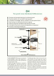
Fig 2: <strong>HYPROP</strong> assembly<br />
Figure 3-1<br />
13/104
Product description<br />
Sampling ring<br />
Silicone gasket<br />
Tensiometer shaft<br />
for lower level incl.<br />
ceramic tip<br />
O-Ring, prevents<br />
intrusion of soil<br />
Tensiometer shaft<br />
for upper level incl.<br />
ceramic tip<br />
O-Ring, seals<br />
Tensiometers<br />
Screw-in thread for the<br />
shafts with pressure<br />
transducer beneath<br />
Fastener clip<br />
Temperature sensor<br />
Sensor unit<br />
Fig. Figure 3: Sensor 3-2 unit<br />
3.2.2 Pressure transducers<br />
The internal pressure transducers measure the soil water tension in<br />
the sample through the two shafts differentially against atmosphere.<br />
14/104
Product description<br />
3.2.3 Tensiometers<br />
Tensiometers measure the soil water tension or the matric potential.<br />
These Tensiometers have a measuring range of +100 kPa<br />
(water pressure) to -85 kPa (water tension). With proper<br />
filling the Tensiometers may work beyond the conventional<br />
tension measuring range. If the soil gets too dry the<br />
Tensiometer needs to be refilled (see chapter “Refilling”).<br />
The soil water tension is conducted via the porous ceramic<br />
tip to the water inside the shaft and measured as an<br />
analogue signal by the pressure transducer.<br />
The Tensiometer shafts are screwed into the transducer<br />
openings in the sensor unit. Standard sampling rings can<br />
Fig 3-3<br />
easily be placed on the sensor unit so the Tensiometer<br />
ceramic tips are positioned inside the soil sample. There is<br />
one short and one long shaft to pick up the tension at two depths.<br />
The Tensiometer shafts are one of the most sensitive parts of the<br />
system. Always handle them with care.<br />
To transfer the soil water tension as a negative pressure into the<br />
Tensiometer, a semi-permeable diaphragm is required. This must<br />
have good mechanical stability and water-permeability, but also have<br />
gas impermeability.<br />
The Tensiometer tip consists of porous ceramic Al 2 O 3 sintered<br />
material. The special manufacturing process guarantees<br />
homogeneous porosity with good water conductivity and very high<br />
firmness. Compared to conventional porous ceramics the tip is much<br />
more durable.<br />
The bubble point of a Tensiometer ceramic is about 800 kPa. If the<br />
soil gets dryer than the bubble point, air passes through. Thus, the<br />
negative pressure inside the cup decreases and the readings go<br />
down to 0 kPa.<br />
With these characteristics this material has outstanding suitability to<br />
work as the semi permeable diaphragm for Tensiometers.<br />
Be aware that the ceramic will dry out when it is exposed to air<br />
uncovered. Always put on the rubber cap filled with some water.<br />
15/104
Product description<br />
3.2.4 Temperature sensor<br />
A temperature probe sits inside the small stainless steel pin on the<br />
sensor unit. It measures the temperature of the soil sample. Although<br />
the temperature is not part of the measurement it is useful<br />
information for reviewing the quality of a measuring campaign. The<br />
sensor has a tolerance of ±0.2 K at 10 °C.<br />
3.2.5 Plug connector<br />
The bus cable is connected to the plug on the side of the sensor unit.<br />
As the plug is taken on and off<br />
regularly during a measuring campaign<br />
an easy-going push-pull plug is used.<br />
A simple-to-open spring-loaded cover<br />
protects the plug when no cable is<br />
connected. Tightly close the plug cover<br />
before cleaning the sensor unit.<br />
Figure 3-4<br />
Dirt water inside the plug opening will destroy the functionality of<br />
the connector.<br />
Do not twist the plug.<br />
Make sure that the cover is closed tightly before cleaning.<br />
3.3 Sampling ring<br />
A soil sample is taken with a stainless-steel sampling ring which has<br />
a volume of 250 ml. The sampling ring is placed on the sensor unit<br />
and fastened with the two clips. A silicone gasket completely seals<br />
the bottom of the soil sample.<br />
3.4 Software tensioVIEW ®<br />
The <strong>HYPROP</strong> system is equipped with the tensioLINK ® measuring<br />
bus.<br />
16/104<br />
Fig. 6: tensioVIEW ®
With tensioLINK ® you<br />
are able to create an<br />
extended network. The<br />
network is connected to<br />
a PC with the<br />
tensioLINK ® USBconverter.<br />
The Windows<br />
software tensioVIEW ® is<br />
used for configuration of<br />
the devices and to<br />
visualize data. The<br />
software automatically<br />
recognizes all connected<br />
devices.<br />
Figure 3-5<br />
Additional functions are integrated in tensioVIEW ® for optimized<br />
usage with <strong>HYPROP</strong> (see chapter ”Performing a measuring<br />
campaign“.). The functions are activated whenever the bus<br />
recognizes that a <strong>HYPROP</strong> unit is connected.<br />
If a laboratory scale with serial RS232 or USB interface is used<br />
readings are automatically taken and evaluated by the tensioVIEW ®<br />
software.<br />
17/104
Get ready to start a measuring campaign<br />
4 Get ready to start a measuring<br />
campaign<br />
The following tools are required to prepare a <strong>HYPROP</strong> unit before a<br />
measuring campaign:<br />
- Sampling ring, volume 250 ml<br />
- Perforated saturation bowl<br />
- A dish or bowl with minimum rim height 7 cm<br />
- Mesh fabric, 15 cm x 15 cm<br />
- Auger positioning tool<br />
- <strong>HYPROP</strong> auger<br />
- Pair of scissors*<br />
- Service case for Tensiometer refilling<br />
* not included<br />
Figure 4-1<br />
18/104
Get ready to start a measuring campaign<br />
4.1 Soil samples<br />
4.1.1 Soil Sampling<br />
Samples should be as fresh as possible. Please follow the guidelines<br />
for taking soil samples (described in DIN 4021, “Exploration by<br />
excavation and borings; sampling)<br />
Following a short instruction for<br />
soil sampling based on lecture<br />
notes from Prof. Dr. W. Durner:<br />
Uncover the preferred soil level.<br />
This can be either vertical or<br />
horizontal. Hammer in the ring<br />
by using a proper knock-on<br />
handle and a medium size<br />
hammer. Hammer in straight<br />
Figure 4-2<br />
19/104<br />
and avoid tilting the ring.<br />
Carefully excavate the ring with<br />
a knife or spatula. Now cut off the overlapping soil along the ring’s<br />
rim with a very sharp knife - take care not to smear the pores. Cover<br />
the samples with protective caps for transportation. In general a<br />
minimum of 5 to 10 samples per soil level are taken to determine the<br />
bulk density and the retention curve.<br />
Weights of the sampling rings might vary. Therefore, it is essential<br />
that the rings are specifically weighed.<br />
4.1.2 Saturate the samples<br />
Remove the protective cap from the upper side of the sample (the<br />
side with the straight rim without cutting edge) and place the mesh<br />
fabric on the sample.<br />
Attach the perforated<br />
saturation attachment to<br />
clamp the cloth.<br />
Turn around the sample and<br />
remove the second plastic<br />
cap.<br />
Fill the dish with water and<br />
place the sample in the dish,<br />
standing on the perforated<br />
attachment.<br />
Figure 4-3
Get ready to start a measuring campaign<br />
Figure 4-4<br />
The water level should be<br />
2 cm in the basket.<br />
Please place the sample<br />
ring incl. saturation bowl<br />
in the basket.<br />
The cutting edge shows<br />
upwards, thus the sample<br />
is saturated capillary from<br />
the reverse side.<br />
After 4-6 h fill new water<br />
inside the basket ca. 1cm<br />
below the upper rim of the<br />
sampling ring.<br />
Important note: Slightly lift up and tilt the sampling ring with<br />
saturation attachment inside the water filled saturation bowl. This<br />
prevents that air bubbles are trapped between soil sample and<br />
mesh fabric. Do this carefully so no soil particles are flushed out.<br />
The duration until the sample is saturated and all air is removed will<br />
depend on the soil type. When saturated, the sample surface will<br />
have a glossy appearance. Clayey soil will need the longest (several<br />
days).<br />
20/104
Get ready to start a measuring campaign<br />
4.2 Filling<br />
Important cautions<br />
Caution: The Hyprop uses highly sensitive pressure transducers.<br />
Improper handling can cause irreversible damage!<br />
Read the chapter about refilling in this <strong>manual</strong> first.<br />
Be extremely cautious when<br />
screwing in the filled<br />
Tensiometer cups. The<br />
pressure inside the cup will<br />
rise abruptly and<br />
exceedingly! Always<br />
observe the pressure in the<br />
online window of<br />
tensioVIEW!<br />
Screw in the shaft slowly,<br />
make sure the pressure<br />
always is below the yellow<br />
range.<br />
Read the complete chapter<br />
about refilling in this <strong>manual</strong>!<br />
21/104
Get ready to start a measuring campaign<br />
Be cautious when pulling off<br />
the tube as vacuum is<br />
inside!<br />
An abrupt negative pressure<br />
change on the water column<br />
might destroy the pressure<br />
transducer.<br />
Do not pull off the tube<br />
rapidly. Allow the pressure<br />
to be released through the<br />
end of the tube or pull off<br />
the tube slowly so the<br />
pressure inside the refilling<br />
adaptor will rise slowly.<br />
Be cautious when tapping<br />
off air bubbles!<br />
Do not knock the sensor<br />
head too hard when under<br />
pressure. Any impact of the<br />
water column might destroy<br />
the pressure transducer.<br />
After finishing the degassing<br />
it is important to remove the<br />
tube by pressing down the<br />
blue ring on the tube<br />
connector. Do not pull out<br />
the tube with force as this<br />
might cause leakage of the<br />
connector.<br />
22/104
Get ready to start a measuring campaign<br />
Before starting and after every completed measuring campaign (the<br />
sample is dried out) the Tensiometers need to be filled or refilled<br />
bubble free with deionised and degassed water. We recommend<br />
degassing and refilling the <strong>HYPROP</strong>-Tensiometers after every<br />
completed measurement campaign. If the measurement is stopped<br />
before the bubble point of the Tensiometers are reached they can be<br />
reused, provided the ceramic is kept moist (plug on the rubber cap<br />
filled with some water).<br />
Two spare Teniometer cups are supplied. Always keep them moist,<br />
because then the degassing and refilling will be quicker.<br />
Keep the ceramic moist when not in use by covering them with the<br />
water filled rubber cap.<br />
Ceramic tip: Do not touch the tip with your fingers. Grease, sweat<br />
or soap residues will influence the ceramic's hydrophilic<br />
performance.<br />
The used Vacuum pump should be able to evacuate 2 kPa closed<br />
to vacuum<br />
The <strong>HYPROP</strong>-service kit or a vacuum system and a PC/Laptop with<br />
tensioVIEW ® software are required for filling or refilling.<br />
23/104
Get ready to start a measuring campaign<br />
4.2.1 Refilling of the <strong>HYPROP</strong><br />
This chapter describes the refilling using a vacuum pump and<br />
<strong>manual</strong> refilling using the tools of the <strong>HYPROP</strong> service kit.<br />
The procedure requires 4 steps, which will be discussed in detail<br />
later in the chapter:<br />
• Degas ceramic cup and shaft<br />
• Degas the sensor unit<br />
• Reassemble<br />
• Check the result<br />
4.2.2 Degas ceramic tip and refill <strong>HYPROP</strong> shaft<br />
If the tip is completely dry just put the empty shaft in a beaker with<br />
de-ionized or distilled water (1,5 cm level) and leave it overnight.<br />
<strong>HYPROP</strong> shafts should<br />
never be filled from the<br />
inside. To avoid that air is<br />
trapped inside the ceramic<br />
the water must flow in one<br />
direction only from the<br />
outside into the interior.<br />
Keep parts clean so there<br />
will be no leaking when<br />
vacuum is applied.<br />
Figure 4-5<br />
24/104
Get ready to start a measuring campaign<br />
Refilling with a Vacuum pump:<br />
Connect rubber tubes to the shafts. Connect the tubes to a vacuum<br />
bottle, and the vacuum bottle to the pump.<br />
Start the pump and evacuate the system for at least 30 minutes and<br />
switch off the pump for 1h. The vacuum drops down slowly, air<br />
bubbles become smaller and can ascend. Repeat this procedure<br />
approximately three times. When water (circa 10 ml) was drawn<br />
through both ceramic tips they are filled.<br />
Figure 4-6<br />
25/104
Get ready to start a measuring campaign<br />
Manually Refilling (incl. delivery):<br />
Alternatively, take the reservoir syringe, fill it with completely<br />
degassed water 1 and take care to avoid bubbles in front of the<br />
ceramic. Fill the shaft with water and plug the vacuum syringe filled<br />
with ¼ deionized degased water completely over the thread. Pull it,<br />
until both snappers are locked. Now, the water from the reservoir<br />
syringe is drawn through the ceramic tip into the vacuum syringe.<br />
When approximately 10 ml are flushed through the ceramic the<br />
<strong>HYPROP</strong> shaft is filled.<br />
Figure 4-7<br />
1 Push out all air from the syringe. Now plug the end of the tube with your finger and<br />
pull up the syringe. This creates vacuum inside the syringe and dissolved gas is<br />
released. Rotate the still evacuated syringe to collect all bubbles from the wall of the<br />
syringe. Hold the syringe upright and slide in the piston. Unblock the tube and push<br />
out all air. Repeat this procedure until no bubbles are produced anymore.<br />
26/104
Get ready to start a measuring campaign<br />
4.2.3 Degas the sensor head<br />
Avoid that the plug connector gets in contact with water.<br />
Take care that the piston never recoils abruptly as this might<br />
damage the pressure transducer (max. 3 bar)!<br />
Please note: new vent cock assembled to the acrylic attachement of<br />
the sensor head .<br />
Figure 4-4 vent cock vertically: closed to ambient air<br />
Figure 4-5 vent cock horizontally: open to ambient air, ventilation of<br />
the sensorhead, but closed to vacuum pump.<br />
Figure 4-8 Figure 4-9<br />
27/104
Get ready to start a measuring campaign<br />
Please fill the two threads<br />
with degased water<br />
carefully with the droplet<br />
syringe…<br />
Figure 4-10<br />
…and fill up the bottom of<br />
the sensor head until the<br />
upper edge.<br />
Figure 4-11<br />
28/104
Get ready to start a measuring campaign<br />
Filling with vacuum pump:<br />
Place the acrylic sensor head attachment onto the sensor head. The<br />
sensor head should sit firmly on the O-Ring. Fill up the acrylic<br />
attachment with deionised water using the droplet syringe up to 1 cm<br />
above the upper edge of the sensor head and connect the tube to<br />
the acrylic sensor head attachement and the vacuum pump.<br />
It is important to know that the vacuum is not applied abruptly. This<br />
can be done very easily with the vent cock. (from open position<br />
(Figure 4-9) to closed position (Figure 4-8))<br />
Manually Refilling:<br />
Take the syringe that belongs to the sensor unit attachment. Draw up<br />
15 ml of water.<br />
Degas the water as described<br />
before and push out all air from<br />
the syringe.<br />
Place the acrylic sensor head<br />
attachment onto the sensor<br />
head. The sensor head should sit<br />
firmly on the O-Ring. Fill up the<br />
acrylic attachment with deionised<br />
water using the droplet syringe<br />
completelly full. (see Fig. 4-8).<br />
Fill the tube with water.<br />
Attach the tube, the vacuum<br />
syringe and the acrylic<br />
attachement<br />
Draw the syringe up until the<br />
black spacer snaps in. Air<br />
bubbles will assemble inside the<br />
Figure 4-12<br />
syringe. To avoid damaging the<br />
pressure transducer, please securely hold the piston so it will not<br />
suddenly recoil. Release the spacers and allow the piston to return<br />
slowly. Only water should flow back into the acrylic attachment. Take<br />
off the tube and push the assembled air out of the syringe. Reattach<br />
the tube and draw the syringe up again until the spacers snap in<br />
(repeat this procedure 3 times. The water now is being degassed.)<br />
We recommend controlling the quality of the vacuum by observing<br />
the refilling window in tensioVIEW<br />
29/104
Get ready to start a measuring campaign<br />
4.2.4 Reassemble the sensor unit<br />
When screwing in the Tensiometer shaft into the thread of the<br />
sensor head it is very important to monitor the pressure in the<br />
refilling window in tensioVIEW ® .<br />
The pressure sensor diaphragm is inside the small hole (ca. ∅2<br />
mm) on the pressure sensor unit. It is very sensitive and must<br />
never be touched! It can be destroyed even by slightest contact (e.<br />
g. with a needle).<br />
No contamination should get on sealing and gasket.<br />
Please connect the <strong>HYPROP</strong> cable and the USB cable to the<br />
sensorhead and start the refilling window in tensioVIEW ®. The<br />
pressure signal should be very closed to zero.<br />
Push the silicone cap (or tube) over the shafts to protect the ceramic,<br />
please don´t touch the ceramic with<br />
your fingers!<br />
Add a drop of water on top of the<br />
shaft with the droplet syringe, so the<br />
meniscus is convex (see Figure 4-9)<br />
Each hole on the sensor unit is<br />
marked by a groove. The long shaft<br />
is inserted where the long groove is,<br />
and the short shaft where the short<br />
groove is.<br />
Figure 4-13<br />
30/104
Get ready to start a measuring campaign<br />
Carefully screw the shaft into the<br />
sensor unit. While screwing (ca 8<br />
turns) in the Tensiometer shaft<br />
the pressure must not exceed 1<br />
bar (burst pressure = 3 bar). In<br />
case the pressure rises to high,<br />
stop the turning in and wait until<br />
the pressure has dropped. You will<br />
clearly notice the point when the<br />
shaft hits the O-ring inside the<br />
sensor unit. From this point do only<br />
another quarter turn!<br />
(1)<br />
Figure 4-14 (2)<br />
On the sensor unit push an O-ring<br />
(1) over each of the shafts (2) to the<br />
very bottom. The rings will keep out<br />
dirt once the Tensiometer shafts<br />
are installed. Place a water filled<br />
silikon tube on the ceramic tip. It is<br />
very important that the ceramic is<br />
always wet.<br />
Repeat the same procedure with<br />
the second <strong>HYPROP</strong> shaft.<br />
Figure 4-15<br />
31/104
Get ready to start a measuring campaign<br />
4.2.5 Check the <strong>HYPROP</strong><br />
Please start again the refilling window.<br />
To check the Zero point, please put a droplet of water onto the<br />
ceramic tip. The values should be around 0 +/- 3 hPa (0,3 kPa)<br />
Wrap a dry paper towel around one ceramic tip to create a<br />
momentary dry ceramic surface. Now create airflow around the<br />
ceramic cup, e. g. by waving a sheet of paper. The reading should<br />
rise to -800 hPa (-80 kPa) within seconds. If this is the case, the<br />
Tensiometer is filled correctly. Do the same with the second tip.<br />
To find out the maximum measuring range of the Tensiometers take<br />
a bottle filled with water and hold the ceramic tip into the headspace<br />
of the bottle. When you move the ceramic away from the water<br />
surface the air gets dryer and the suction rises.<br />
Hold the ceramic close to the water surface so the tension reading<br />
will rise slowly. Depending on the filling quality the value will reach<br />
-85 to -450 kPa. Then, the value will rapidly drop to the vapor<br />
pressure (around -90 kPa depending on the altitude). Now<br />
immediately put some water on the ceramic and cover the ceramic<br />
with the protective rubber cap which should be halfway filled with<br />
water. It will take one day until the Tensiometer will reach its initial<br />
value.<br />
32/104
Get ready to start a measuring campaign<br />
4.3 Attach the sampling ring<br />
Take the saturated soil sample out of the saturation dish. Place the<br />
auger positioning tool on the sampling ring as shown in the picture..<br />
Insert the auger into each opening<br />
and drill a hole in 3 steps (to avoid<br />
compressing the soil). Drill as far as<br />
the auger will go. Rotate the auger<br />
while pulling it out of the sample.<br />
Then, you will have 2 holes in the<br />
sample, each with the proper depth.<br />
With a pen make a mark on the side<br />
of the sampling ring where the<br />
deeper hole is (see Figure 4-12).<br />
Then you know the correct position<br />
when placing the sample on the<br />
sensor unit<br />
Figure 4-16<br />
To avoid that air will be pressed<br />
inside the sample it is<br />
recommended to fill up the holes<br />
with water. (see Figure 4-17 ).<br />
The sample now is ready for<br />
attaching the sensor unit.<br />
Wipe off the ring surface after<br />
having drilled the holes.<br />
Figure 4-17<br />
Watch your mark. The long shaft must be inserted into the deeper<br />
hole. Keep the ceramic tips wet!<br />
If the soil sample swelled up during saturation the overlapping soil<br />
must be cut off before attaching the sensor unit.<br />
33/104
Get ready to start a measuring campaign<br />
Remove the protetion tube from the ceramic tip. Place the silicone<br />
gasket on the bottom of the sensor head (mud protection).<br />
Turn the sensor unit up side down<br />
and carefully place it on the soil<br />
sample by inserting the<br />
Tensiometer shafts into the drilled<br />
holes. Please take care that no air<br />
gaps and soil compression will<br />
happen.<br />
Now turn the assembly and remove<br />
saturation bowl and cloth. Close the<br />
clips to fix sampling ring and sensor<br />
unit.<br />
Figure 4-18<br />
Figure 4-19<br />
Figure 4-20<br />
34/104
Set-up the <strong>HYPROP</strong><br />
5 Set-up the <strong>HYPROP</strong><br />
In the next step please place the sensor head on the tared scale and<br />
plug in the cables.<br />
Figure 5-1<br />
5.1 Connect the system components<br />
The next step is to connect the components with tensioLINK ® .<br />
Up to 20 sensor units can be linked to a PC at the same time with<br />
the supplied bus cables and distributors.<br />
Above (Figure 5-1) the sensor unit is directly connected to the PC<br />
with the <strong>HYPROP</strong> USB-converter. The internal power supply of the<br />
USB-converter is capable of powering a single sensor unit. (please<br />
be aware to set the PC to constant power mode)<br />
35/104
Set-up the <strong>HYPROP</strong><br />
Figure 5-2<br />
In the multi device mode connect each sensor unit to a T-piece plug<br />
with a <strong>HYPROP</strong> connecting cable. Sensor units can be connected in<br />
any order as the software recognizes the position of any sensor unit<br />
automatically.<br />
Finally connect the main power supply unit to the plug of the last T-<br />
piece plug and the <strong>HYPROP</strong> USB converter to a free USB port on<br />
your PC. The internal power supply of the USB-converter is capable<br />
of powering a single sensor unit. As soon as 2 or more sensor units<br />
are connected the USB-power supply is not sufficient. Therefore, the<br />
main power supply unit should always be connected.<br />
36/104
Set-up the <strong>HYPROP</strong><br />
In the single device mode the <strong>HYPROP</strong> assembly remains on the<br />
scale and the USB-cable is connected all the time. Therefore, it is<br />
important to stabilize the USB-cable. A proper stabilization for the<br />
USB-cable is required. Even smallest movements of the cable can<br />
cause erroneous measurements. (see more next chapter)<br />
Figure 5-3<br />
37/104
Set-up the <strong>HYPROP</strong><br />
5.1.1 Scale<br />
A laboratory scale with interface is required. If the type of scale is not<br />
in the following list, the scale is not supported and has to be send in<br />
to <strong>UMS</strong> (incl. <strong>manual</strong> and interface cable).<br />
Supported scales:<br />
Kern EG2200 (recommended)<br />
Kern EW3000<br />
Kern 572<br />
CHYO MK2000B<br />
Mettler Toledo SICS<br />
Mettler Toledo PM2000<br />
COBOS COBOS-CB Complet<br />
If the scale has a serial RS232 interface connect it to a free COMport<br />
on your PC. You can use a RS232-USB-converter if no COMport<br />
is available on your PC. Please carefully follow the instructions<br />
for the RS232-USB-converter.<br />
The set-up of the scale in tensioVIEW® is described in chapter 5.3<br />
„Add the Scale“<br />
Figure 5-4<br />
38/104
Set-up the <strong>HYPROP</strong><br />
Please note the following requirements for the operation of the scale<br />
(also see 6.1 Starting conditions p 50):<br />
1. The scale should be placed on a vibration-free work table.<br />
2. The work table should only be used for the <strong>HYPROP</strong><br />
measurement.<br />
3. The scale must be levelled out. Most scales have a bubble-level.<br />
4. Since the Earth's gravity varies at each location the balance has<br />
to be calibrated before the initial operation and every time the<br />
balance is relocated. A periodical recalibration is recommended.<br />
Use a standard weight of accuracy class M1. Please read and<br />
follow the instructions in the <strong>manual</strong> of the balance. The<br />
recommended scale Kern EG 2200 has an internal precision<br />
weight, thus the accuracy of the balance can be checked at any<br />
time and adjusted.<br />
5. The weight, marked on the samping rings, relates to a gravity of<br />
9,802 ms-2. The gravity mainly depends on the latitude<br />
9,780(0°) -9,833 (90°) ms-2.<br />
6. Cable fixation<br />
To avoid errors the <strong>HYPROP</strong> cable must be fixed. Mount the<br />
<strong>HYPROP</strong> sensor cable as shown in the picture below. Clip the<br />
cable into the cable clips. The cable should be put on the scale<br />
and tared to “0”<br />
Figure 5-5<br />
39/104
Set-up the <strong>HYPROP</strong><br />
Figure 5-6<br />
Cable length between plug and upper cable clip should be about 15<br />
cm.<br />
Cable length of the loop between both cable clips should be about 20<br />
cm.<br />
If you don´t have this clips please ask us for the accessory kit (incl<br />
Application Note) to fix the cable. It is free of charge.<br />
40/104
Set-up the <strong>HYPROP</strong><br />
5.2 Software tensioVIEW ®<br />
5.2.1 Menu<br />
tensioVIEW ® has simple, mostly self-explaining menus for read-out<br />
and configuration of tensioLINK devices.<br />
After starting tensioVIEW ® the display is more or less blank, most<br />
functions are not activated.<br />
5.2.1.1 Find devices<br />
If one or more sensors are connected via the USB-converter<br />
they can be found by pressing the “magnifying glass” button.<br />
tensioVIEW ® offers two options for searching:<br />
5.2.1.2 Single device mode<br />
tensioVIEW ® expects that only one device is connected which<br />
will be found very quickly. This mode is not functional if more<br />
than one device is connected!<br />
5.2.1.3 Multiplexed devices mode<br />
tensioVIEW ® is able to run up to 20 <strong>HYPROP</strong> sensor units<br />
connected to the bus within 8 seconds, but only if each device<br />
is already personalized with an individual bus identification address.<br />
If two or more devices have an identical address, none of them will<br />
be found.<br />
All devices found will be displayed in the left section in a directory<br />
tree. Same types of devices will be grouped in one directory.<br />
41/104
Set-up the <strong>HYPROP</strong><br />
Double-click on the device<br />
5.2.2 Device window<br />
Figure 5-7<br />
Detected devices will be displayed with their programmed names.<br />
Press the + symbol to see what readings parameter are available.<br />
Double-click on the name to open a menu window where all<br />
specifications and functions of this device are displayed. Depending<br />
on the type, different registries are available. The first shows an<br />
overview of the current settings and information about address<br />
number or error messages.<br />
5.2.2.1 Properties<br />
Gives an overview about the sensor head’s basic properties and is<br />
only informative. You cannot edit the properties in this window.<br />
5.2.2.2 Configuration of a device<br />
Select the tab "Configuration“ for viewing and changing the<br />
programmed settings of the device.<br />
42/104
Set-up the <strong>HYPROP</strong><br />
Depending on the authorization status, only parameters that can be<br />
edited are shown. To store a changed parameter in the device it has<br />
to be sent to the device by pressing the "Upload“ button. A message<br />
confirming the successful configuration will be displayed.<br />
Configuration changes are effective immediately.<br />
Figure 5-8<br />
43/104
Set-up the <strong>HYPROP</strong><br />
5.2.2.3 Configuration settings for <strong>HYPROP</strong><br />
Those settings which are editable only for Power users are marked<br />
with an asterisk *.<br />
Parameters with related functions are bundled in one folder.<br />
tensioLINK<br />
Bus number<br />
tensioLINK ® bus number of the device<br />
Sub address<br />
tensioLINK ® sub address of the device<br />
Explanation:<br />
tensioLINK ® uses two types of address for each device, the bus<br />
address and the sub address. The reason for this is that is there<br />
might be sensors installed at the same spot, but with different<br />
measuring depths (for example multi-level probes). In this case, the<br />
sub address defines the depth starting with 1 for the highest sensor.<br />
Furthermore, the sub address could be used to combine groups of<br />
sensors, for example of one measuring site.<br />
In general the required identification for a device is always the bus<br />
number. If more than 32 devices are connected to the bus the sub<br />
address is counted up. The allowed numbers for the bus address are<br />
1 to 32 and for the sub address 1 to 8.<br />
The default value for both bus and sub address is 0. With more than<br />
one device connected individual addresses have to be declared.<br />
Device Info<br />
Name<br />
Individually editable name of the Tensiometer in ASCII. Maximum<br />
length 12 digits<br />
Measure head net weight<br />
is the net weight of the sensor head incl. Tensiometer shafts and<br />
silicone disc.<br />
* User rights are selected in the bottom status line. Select between „Public“<br />
(limited rights) und „Power“ (extended rights). The software needs to be<br />
restarted when this setting is changed.<br />
44/104
Set-up the <strong>HYPROP</strong><br />
Soil volume<br />
Volume of the soil sample in the sampling ring excluding the<br />
Tensiometer shafts’ volume.<br />
Soil column height<br />
Height of the soil column in mm (height of sampling ring).<br />
Depth lower tens<br />
Protruding length of the lower shaft.<br />
Depth upper tens<br />
Protruding length of the upper shaft.<br />
Data logger<br />
Interval<br />
the logging interval of the internal data logger<br />
Overwrite old values<br />
Overwrites old values (if you select „on“) if the memory is full<br />
Sensor measuring<br />
Continuous measuring<br />
Activate the quick updating of readings to receive the <strong>HYPROP</strong><br />
readings instantly, for example during a refilling procedure.<br />
Measurements are taken in intervals of 50 ms. Note the rise in power<br />
consumption and that the reaction to serial commands might be<br />
slowed down. The setting "Measuring interval“ is deactivated during<br />
this mode..<br />
Measuring interval<br />
This is the standard interval in which sensor measurements are<br />
refreshed and available on the analogue lines.<br />
Enable filter<br />
Activate the anti-flicker-filter. This avoids that the digit continuously<br />
jumps up and down. When activated the resolution is reduced for<br />
one digit.<br />
45/104
Set-up the <strong>HYPROP</strong><br />
5.2.3 Refilling window<br />
This function is required when the <strong>HYPROP</strong> sensor head needs to<br />
be refilled or during assembly of sensor head and Tensiometer<br />
shafts (strictly recommended!!).<br />
When the Tensiometer shafts are screwed back into the sensor<br />
unit the pressure reading must be checked at any time to avoid<br />
that excess pressure destroys the pressure transducer. Stop or<br />
slow down if the pressure rises to much. Please read the chapter<br />
4.2 ”Refilling“ for more details.<br />
Figure 5-9<br />
46/104
Set-up the <strong>HYPROP</strong><br />
5.2.4 Current readings<br />
In this window you can display current values of the Tension Bottom<br />
, Tension top and Temperature, depending on the Parameter<br />
Interval.<br />
5.2.5 Stored readings<br />
In this window you can download stored readings and delete stored<br />
readings, if logged data is available!<br />
47/104
Set-up the <strong>HYPROP</strong><br />
5.3 Add the scale<br />
Before you can start a measuring campaign the scale needs to be<br />
added to the system. As scales have different specifications no<br />
automatic search is implemented in the program. Only scales<br />
supplied by <strong>UMS</strong> are pre-set.<br />
There are two ways to add a new scale:<br />
1. Click the right mouse button on <strong>HYPROP</strong> in the parent directory<br />
to open the “Add“ and “Add <strong>HYPROP</strong> device“ window. Click on<br />
„Add new Scales“.<br />
2. Select the button in the menu
Set-up the <strong>HYPROP</strong><br />
Select the scale type, for example “Kern EG2200“, the interface and the<br />
connection parameters. Then click on the Measure-Button. If a<br />
connection is established „zero“ is displayed for both status and<br />
reading. Click “OK“ to select the scale.<br />
Now the new device is shown in the explorer window.<br />
Figure 5-11<br />
If you click on “Scale“ in the explorer window the current readings<br />
are shown.<br />
49/104
Perform a measuring campaign<br />
6 Perform a measuring campaign<br />
Definition: a measuring campaign comprises the set-up<br />
configuration, tension readings, weight readings and the evaluation<br />
of one <strong>HYPROP</strong> assembly or of all assemblies measured at the<br />
same time. This information is stored in one file for further use.<br />
Familiarise yourself with the functions of tensioVIEW ®<br />
start a measuring campaign.<br />
before you<br />
The starting conditions for a campaign are extremely important<br />
Always power a laptop with a mains power unit, not just only by<br />
battery.<br />
It is extremely important that the cable is not moved during a<br />
measurement campaign. Securely fix the cable as even a breeze<br />
can move a dangling cable causing variance in the measurement.<br />
Avoid leaving water drops on the fastener clips.<br />
6.1 Starting conditions<br />
The following conditions must be fulfilled before a measurement can<br />
be started:<br />
1. The initial water content of the<br />
completely saturated sample is<br />
estimated. It can be calculated if<br />
the soil type is definitely known<br />
2. The sample must be protected<br />
from direct sunlight, air currents<br />
or extreme temperature<br />
changes.<br />
Figure 6-1<br />
50/104
Perform a measuring campaign<br />
3. The scale should be placed on a vibration-free work table. The<br />
work table should not be used for other purposes during a<br />
<strong>HYPROP</strong> measurement.<br />
4. During a single mode measurement we strictly recommend to fix<br />
the cable of the sensor unit.<br />
5. The scale must be levelled out. Most scales have a bubble level.<br />
6. Set the energy manager of your laptop to non-stop operation.<br />
Open the energy option manager and set „Power-down“ and<br />
„Stand-by“ to „Never“. If the laptop powers down or goes to the<br />
stand-by mode no readings are stored.<br />
51/104
Perform a measuring campaign<br />
6.2 Measuring campaign window<br />
There are two ways to open the measuring campaign window.<br />
1. In the menu bar select <br />
2. Click this button:<br />
Figure 6-2<br />
52/104
Perform a measuring campaign<br />
6.3 Configure the campaign<br />
Open the measuring campaign window to configure the system.<br />
Enter file name and directory where you want to store the measuring<br />
campaign:<br />
Under enter the starting time of the campaign<br />
and the intervals when to weigh the samples (fig. below)). Select<br />
if the campaign only includes one assembly.<br />
Higher frequency means: a<br />
measuring interval of 1<br />
minute at the beginning of<br />
the measurement<br />
In the units menu select the units for tension, conductivity and matric<br />
potential. Select either logarithmic or linear display.<br />
In the window the device name and serial number is<br />
displayed automatically.<br />
Soil sampling ring weight (default 201g), and sample name need to<br />
be entered.<br />
53/104
Perform a measuring campaign<br />
6.4 Perform the measurement<br />
6.4.1 Single unit mode and multiplex device mode<br />
In general there are two modes, the single unit mode and the<br />
multiplex devices mode. The following table shows the differences.<br />
Single unit mode Multiplex device<br />
mode<br />
Sensor unit 1 2-20<br />
Symbol<br />
Weighing<br />
Measuring time<br />
remains on the scale<br />
continuously<br />
the selected<br />
measuring time is<br />
also the weighing<br />
interval<br />
you are asked to<br />
place each unit on<br />
the scale according<br />
to the measuring<br />
cycle<br />
you set the time<br />
separately<br />
6.4.2 Start of a measuring campaign<br />
Click the button „Start Campaign“ to start the<br />
measuring campaign. The intervals entered in<br />
the configuration are assumed.<br />
6.4.3 Constant starting conditions<br />
When you set the start line there must be constant starting<br />
conditions. This means that the tension values are constantly<br />
horizontal for a certain time period (preparation of the sample and<br />
hardware see chapter 6.1 ).<br />
54/104
Perform a measuring campaign<br />
6.4.4 Start a spontaneou measurement<br />
In the function window you can optionally click on to<br />
start a measurement spontaneously (out of the constant<br />
measurement).<br />
6.4.5 Current status of the measurement<br />
In the left upper window (”Current status“) the current readings are<br />
displayed.<br />
Anytime you can stop the campaign, change the interval or restart<br />
the campaign. The logging is continuously, starts and stops are<br />
marked with a dotted line in the graphs. The upper graph shows the<br />
tensions, the lower graph the weight.<br />
The readings are displayed in a table on the right side of the graphs.<br />
55/104
Perform a measuring campaign<br />
6.4.6 Measurements in the „Single device mode“<br />
Select “Single device mode” under “General Parameters” in the<br />
configuration window. Set up the parameters as described in<br />
the previous chapters. In the single device mode only one measuring<br />
interval is entered which is used for both tension and temperature<br />
measurement.<br />
Start the measuring campaign and do a zero set as described in<br />
chapter ”Zero Set”.<br />
Figure 6-3<br />
56/104
Perform a measuring campaign<br />
Figure 6-4<br />
6.4.7 Multiplex devices mode<br />
Connect all devices with tensioLINK ® to the <strong>HYPROP</strong> main<br />
unit. Click on “Multiplex devices mode” to start a scan. Note<br />
that a different tensioLINK address is given to each device (see<br />
chapter ”Configuration Settings”).<br />
Enter an interval for the Tensiometer measurements, for example 10<br />
minutes.<br />
The interval for weighing can be different than the one for tension<br />
measurement. As the weight of the sample changes slowly it is<br />
recommendable to choose a larger interval (depending on the soil<br />
type). For cohesive soils (clayey soil) we recommend an interval of 3<br />
weight measurements per day. For less cohesive soils (sandy soil) 1<br />
weight measurement per day is sufficient.<br />
At the end of each interval you are asked to measure the samples.<br />
To do so unplug the LEMO plug from the sensor unit. The system<br />
57/104
Perform a measuring campaign<br />
will automatically recognize which sample is put on the scale. The<br />
number of samples is limited to 20.<br />
A new menu opens on the screen showing information about the<br />
status and the routine of the weighing.<br />
Follow the given instructions (fig. 49).<br />
Figure 6-5<br />
6.4.8 Interrupt a measuring campaign<br />
A measurement can be interrupted temporarily as the readings are<br />
stored. Reload them with „Open project“ in the main tensioVIEW<br />
menu (also for example after a power breakdown).<br />
58/104
Perform a measuring campaign<br />
6.5 Description of an ideal measured curve<br />
Each measurement proceeds in 3 phases (provided that<br />
Tensiometers and sensor unit have an excellent filling).<br />
Phase 1: Boiling retardation<br />
The Tensiometer readings rise without flattening into the range of<br />
boiling retardation (beyond -85 kPa).<br />
Phase 2: Consolidation<br />
Water vapor accumulates. The Tensiometer reading abruptly drops<br />
down to the boiling point of approximately -85 kPa and remains<br />
constant at this level (dot and dash line in figure ....).<br />
Phase 3: Air entry<br />
The Tensiometer reading abruptly drops to 0 kPa as air enters the<br />
ceramic cup. The bubbling point of this ceramic is about -880 kPa<br />
(close to pF 4). This value is also used for the evaluation (see<br />
chapter “7 Evaluation”).<br />
Phase 1 2 Phase 3<br />
Figure 6-6: the different phases of the upper Tensiometer (left curve)<br />
59/104
Perform a measuring campaign<br />
6.6 Conclusion of a measurement<br />
A measurement campaign can be concluded if the 1st Tensiometer<br />
(T1) drops to 0 kPa (bubble point) and the 2nd Tensiometer is in<br />
Phase 1 (dash and dot line in Figure 6-7).<br />
Ab hier Abbruch<br />
T1<br />
T2<br />
Figure 6-7<br />
60/104
Perform a measuring campaign<br />
If the 1st Tensiometer (T1) drops to 0 kPa (air entry) and the 2nd<br />
Tensiometer is still in Phase 2 no averaging is possible. In this case<br />
you must wait until the 2nd Tensiometer (T2) reaches the bubble<br />
point. Then, the measurement can be concluded (see Figure 6-8).<br />
Ab hier Abbruch<br />
T1<br />
T2<br />
Figure 6-8<br />
If an extraordinary error occurs the measurement can be stopped<br />
any time.<br />
Exemplary measurements for various soils are shown in the<br />
appendix.<br />
61/104
Perform a measuring campaign<br />
6.7 Remove the soil sample<br />
1. Hold the whole assembly over a bowl or dish to assure that no soil<br />
material is lost.<br />
2. Unlock the fastener clips. Gently pull on the soil sampling ring to<br />
take off the ring from the sensor head.<br />
Figure 6-9<br />
If the soil is too dry and if it is not possible to dismantle the <strong>HYPROP</strong><br />
with the soil (e.g. clay) it is recommended to take the sample in water<br />
to get saturated over night.<br />
62/104
Perform a measuring campaign<br />
3. Please clean the sample ring and the silicon disc above the bowl.<br />
It is more easy to take a brush (see pictures below)<br />
Abbildung Figure 6-11 6-4 Abbildung Figure 6-10 6-5<br />
4. Clean the sensorhead with water (wash bottle) and a dustfree<br />
tissue over the bowl.<br />
63/104
Perform a measuring campaign<br />
5. In the end you should clean the sensor head and the tensiometer<br />
under running water (see picture below)<br />
Figure 6-12<br />
Please unscrew the both <strong>HYPROP</strong> shafts only when the sensor<br />
head is completely clean.<br />
64/104
Perform a measuring campaign<br />
6.8 Dry weight<br />
Empty the soil sample into a bowl with known weight. Dry it in a<br />
drying oven at 105°C for 24 hours and then weigh it again.<br />
Figure 6-13<br />
The „Soil dry weight“ will be used to calculate the actual water<br />
content and has to be entered later in the <strong>HYPROP</strong> FIT Software.<br />
65/104
Evaluation<br />
7 Evaluation<br />
Evaluate a measurement with the <strong>HYPROP</strong>-FIT software.<br />
To execute the evaluation in the correct order proceed<br />
through the menus „Information“, „Messung“, „Auswertung“, „Fitting“<br />
and „Export“ step-by-step.<br />
All options of the software as well as background information about<br />
evaluation and data fitting can be found in the extensive online<br />
<strong>manual</strong> of <strong>HYPROP</strong>-FIT (click on ‘Help’ in the status line).<br />
66/104
Trouble shooting<br />
8 Trouble shooting<br />
Problem<br />
1. It is not possible to achieve a<br />
bubble free filling.<br />
Possible cause and solution<br />
If the tip is completely dry just put<br />
the empty shaft in a beaker with<br />
deionised or distilled water<br />
overnight.<br />
2. The Tensiometer readings only<br />
rise very slowly<br />
3. The Tensiometer reaches a<br />
maximum of -50 kPa, then the<br />
reading drops<br />
4. The Tensiometer shows readings<br />
beyond vacuum (-100 kPa)<br />
a) Could depend on the soil type:<br />
for example sand has a poor<br />
conductivity. Thus, the curve of<br />
the readings will be flatter than<br />
for example in a clayey soil.<br />
b) The Tensiometer is not<br />
sufficiently filled and degassed<br />
(see 1)<br />
c) A leakage has occurred (see 3)<br />
The Tensiometer is not sufficiently<br />
filled and degassed (see 1).<br />
The shaft was not properly screwed<br />
onto the pressure body, and the O-<br />
ring is not tight. Reassemble the<br />
shaft.<br />
This is no error but a particular<br />
feature of the miniature<br />
Tensiometer. Due to boiling<br />
retardation it is possible that the T5<br />
might reach values up to -140 kPa.<br />
Please check fig. 51 for this effect.<br />
5. The curve cannot be fitted a) Reset start and stop line as<br />
described in the chapter „End of<br />
the measuring campaign“.<br />
b) The curve progression is not<br />
consistently rising, eventually it<br />
is necessary to start a new<br />
measurement (causes see<br />
point 3)<br />
6. The recording of readings has<br />
stopped<br />
7. Tensiometer reach only -50 to -70<br />
kPa, then readings drop slowly<br />
Check the USB connections<br />
In the power management menu of<br />
your PC or laptop disable the power<br />
down and select non-stop operation.<br />
67/104<br />
The Tensiometer was not<br />
sufficiently filled. A bubble<br />
assembles inside the ceramic part
Trouble shooting<br />
8. At the beginning the lower<br />
Tensiometer surpasses the upper<br />
one which would indicate a negative<br />
conductivity<br />
9.No sensor units are found in the<br />
multiplex device mode<br />
and interrupts the water contact<br />
(see point 3)<br />
This is caused by inaccuracy of the<br />
sensors. Execute the “Zero offset“ to<br />
compensate the water column shift.<br />
Eventually set the starting point to a<br />
later point.<br />
Disconnect all sensor units. Connect<br />
just one unit and start a search in<br />
the single device mode. Check for<br />
each sensor unit that no address is<br />
given twice (see pages 42/43). In<br />
case, change the address as<br />
described in this <strong>manual</strong>. Sensor<br />
units can only be found if addresses<br />
are unique.<br />
68/104
Service and maintenance<br />
9 Service and maintenance<br />
9.1 Check the <strong>HYPROP</strong><br />
1. First check if the Tensiometers of the <strong>HYPROP</strong> need to be refilled<br />
(recommended always at initial use and after a complete<br />
measurement campaign):<br />
Connect the sensor unit with adapter cable and USB-converter to<br />
your PC and start tensioVIEW ® .<br />
2. Click on the magnifying glass symbol to search for devices.<br />
Select the sensor unit you want to check.<br />
3. Click on “Refilling” to open the<br />
“Refilling window”.<br />
9.1.1 Check the Zero point<br />
If the tips are moist both readings<br />
should be around 0 hPa (between -<br />
5 and + 5 hPa).<br />
If you have not done the zero set<br />
(compensation of water column) the<br />
values are higher due to the shaft<br />
length.<br />
9.1.2 Check the Response<br />
Wrap a dry paper towel around one ceramic tip to create a<br />
momentary dry ceramic surface. Now create an air current around<br />
the ceramic cup, e. g. by waving a sheet of paper. The reading<br />
should rise to -80 kPa within seconds. If this is the case, the<br />
Tensiometer is filled correctly. If not, the Tensiometers needs to be<br />
refilled.<br />
Do the same with the second tip.<br />
69/104
Service and maintenance<br />
9.1.3 Calibration<br />
When delivered the <strong>HYPROP</strong> transducers (Tensiometers) are<br />
calibrated with an offset of 0 kPa (when in horizontal position) and a<br />
linear response. The offset of the pressure transducer has a minimal<br />
drift over the years. Therefore, we recommend to check the<br />
<strong>HYPROP</strong> sensor unit once a year and re-calibrate them every two<br />
years.<br />
Return the <strong>HYPROP</strong> sensor unit to <strong>UMS</strong> for recalibration If<br />
necessary.<br />
9.1.4 Check the Offset<br />
Screw off the Tensiometer shafts. Carefully blow out remaining water<br />
from the shaft drillings. Connect the sensor unit to tensioVIEW ® and<br />
continuously observe the readings.<br />
Wait until the readings are stable. The readings should be between<br />
-0.2 kPa and +0.2 kPa. If the readings are beyond this range a recalibration<br />
might be necessary.<br />
9.2 Cleaning<br />
The sensor unit is rated IP65 and can be cleaned under running<br />
water, but pay attention that the cover of the plug connector is<br />
closed.<br />
Clean ceramic and shaft only with a moist towel. If the ceramic is<br />
clogged it may be flushed with Rehalon®.<br />
If the pores are clogged with clay particles saturate the ceramic and<br />
then polish the ceramic surface with a wetted, waterproof sandpaper<br />
(grain size 150...240).<br />
9.3 Storage<br />
If the <strong>HYPROP</strong> should not be used for a year or more empty shaft<br />
and sensor head to avoid algae growth. Store both in a dry place.<br />
70/104
Service and maintenance<br />
9.4 Change the O-ring on the <strong>HYPROP</strong> sensor unit<br />
After many refilling procedures, but also if the O-ring is squeezed too<br />
hard with the shaft, the O-ring can be worn out, and is not sealing<br />
anymore.<br />
You will notice this if the Tensiometer does not reach the boiling<br />
point anymore (i.e. close to 90 kPa), or the tension curve gets flat or<br />
drops abruptly at a point far below the boiling point (see figure<br />
below).<br />
71/104
Service and maintenance<br />
For replacing the O-ring a pair of fine pointed tweezers is required.<br />
CAUTION: Do not insert the tip into the boring as you might punch<br />
the membrane of the pressure transducer..<br />
How to proceed:<br />
Pierce into the O-ring to pick it<br />
up and remove it.<br />
Spare O-rings can be find in the<br />
service case.<br />
Grab the replacement O-ring,<br />
but now not pierce it. Carefully<br />
insert the ring into the round<br />
groove inside the boring.<br />
If the ring does not slip into the<br />
groove carefully screw in the<br />
shaft to push the ring into its<br />
position.<br />
72/104
Theoretical basics<br />
10 Theoretical basics<br />
10.1 Evaporation method (overview)<br />
In a soil sampling ring two Tensiometers, comparable to the T5<br />
model, are installed in two depths (z 1 and z 2 ). The middle between<br />
the sensing tips of the Tensiometers is the centre of the soil sample.<br />
The sample is saturated, closed on the bottom and placed on a<br />
scale. The upper side of the sample is open to atmosphere so the<br />
soil moisture can evaporate. With the soil water tension [kPa] the<br />
average matric potential and the hydraulic gradient is calculated. The<br />
mass difference, measured by the scale, is used to calculate the<br />
volumetric water content and the water’s flow rate.<br />
A measuring campaign will last until one of the Tensiometers runs<br />
dry or the mass changes become marginal. Then, the remaining<br />
moisture content is determined by oven drying the sample at 105°C<br />
for 24 hours. With these values the retention curve and the<br />
unsaturated conductivity is extrapolated.<br />
10.2 Discrete data for retention and conductivity<br />
relation<br />
At different points of time t i<br />
i<br />
the water tensions h 1<br />
and h i<br />
2<br />
(in hPa) of<br />
both depths are measured as well as the weight of the sample (in<br />
grams ≅ cm 3 ). The analytic procedure is based on the assumption<br />
that water tension and water content distribute linear through the<br />
column, and that water tension and sample weight changes are<br />
linear between two evaluation points.<br />
The initial water content is determined from the total loss of water (i.<br />
e. evaporation + water loss by oven drying).<br />
i<br />
The average water contentθ , derived from initial water content and<br />
i<br />
loss of weight, and the medial water tension h give a discrete value<br />
i ( i<br />
i<br />
θ h ) of the retention function at any time t .<br />
For the calculation of the conductivity function it is assumed that<br />
i−1 i<br />
between two time points t and t the water flow through the cross<br />
73/104
Theoretical basics<br />
section situated exactly between both Tensiometers (and therefore<br />
i<br />
i i<br />
exactly at column centre) is q ( ∆V<br />
∆t<br />
A)<br />
∆V<br />
i<br />
= ½ .<br />
i<br />
∆ t is<br />
is the water loss in cm³ determined by weight changes,<br />
the interval between two evaluation points, and A the cross section<br />
area (in cm²) of the column.<br />
The data for the hydraulic conductivity function are determined by<br />
inverting the Darcy-Equation:<br />
i<br />
K ( h<br />
i−1<br />
i−1<br />
i i<br />
( h + h + h h )<br />
i<br />
h = ¼ 1 2 1 + 2<br />
i<br />
evaluation points, with<br />
cm h -1 ).<br />
i<br />
i (<br />
−1<br />
i−1<br />
i i<br />
∆h<br />
= h − h ) + ( h − h ))<br />
½ 2 1 2 1<br />
i<br />
) = −<br />
∆h<br />
i<br />
i<br />
q<br />
.<br />
/ ∆z<br />
+ 1<br />
is the medial water tension between two<br />
K as the related hydraulic conductivity (in<br />
is the medial difference of the water<br />
tension between both Tensiometers, whereas ∆ z = z 2<br />
− z1<br />
is the<br />
distance between both Tensiometers (in cm).<br />
Unreliable K (h)<br />
data sets close to saturation are filtered depending<br />
to the measuring accuracy of the Tensiometers.<br />
To get a sufficient number of data points for the hydraulic function<br />
even with relatively long intervals, both the tension curve and the<br />
weight curve between two evaluation points are interpolated with<br />
hermitian splines (Peters and Durner, 2008). On this basis relatively<br />
short evaluation intervals are achieved.<br />
10.3 Retention and conductivity functions<br />
Normally hydraulic characteristics are described by parametric<br />
functions for<br />
θ (h)<br />
and<br />
K(h)<br />
.<br />
With <strong>HYPROP</strong> three models can be chosen. These models can be<br />
adapted to measure data via a robust and non-linear optimizing<br />
procedure.<br />
74/104
Theoretical basics<br />
10.3.1 The van Genuchten/Mualem modell<br />
With this model the effective saturation Se<br />
= ( θ −θr<br />
) ( θs<br />
−θr<br />
) and<br />
the unsaturated conductivity K in relation to the matric potential h are<br />
predetermined by the following equation formula (van Genuchten,<br />
1980):<br />
n 1 / n−1<br />
S ( h)<br />
= (1 + ( α h ) )<br />
K(<br />
h)<br />
= K<br />
s<br />
e<br />
(1 + ( α h )<br />
)<br />
n τ (1/ n−1)<br />
n−1<br />
n 1/ n−1<br />
[ 1−<br />
( α h ) [ 1+<br />
( α h ) ] ] 2<br />
Here the residual water content θ r<br />
, the water content at saturation<br />
θ s<br />
, the inverse value of the bubble point potential α [cm -1 ] and the<br />
pore size distribution n [-] are the fitting parameters for the retention<br />
function. Furthermore, the tortuosity parameter τ [-] and the<br />
saturated conductivity<br />
K are fitted to get the conductivity function.<br />
s<br />
10.3.2 The bimodal van Genuchten/Mualem Model<br />
This model suggested by Durner (1994) describes the retention and<br />
conductivity function by overlapping of two individual van Genuchtenfunctions<br />
(Priesack and Durner, 2006).<br />
⎡<br />
K(<br />
h)<br />
= K<br />
s ⎢<br />
⎣<br />
2<br />
∑<br />
j=1<br />
S ( h)<br />
=<br />
e<br />
w [1+<br />
( α h )<br />
j<br />
j<br />
2<br />
∑<br />
j = 1<br />
]<br />
ω (1 + ( α h )<br />
τ<br />
n 1/ n −1<br />
⎤<br />
j j<br />
j<br />
⎥<br />
⎦<br />
⎡<br />
⎢<br />
⎢<br />
⎢<br />
⎢<br />
⎣<br />
2<br />
∑<br />
j=1<br />
j<br />
j<br />
j<br />
n<br />
j<br />
1/<br />
)<br />
n −1<br />
w α {1−<br />
( α h )<br />
j<br />
j<br />
2<br />
∑<br />
j=1<br />
n<br />
j<br />
−1<br />
w α<br />
j<br />
[1+<br />
( α h )<br />
j<br />
j<br />
n<br />
j 1/ n j −1<br />
The j are indexes for the parameters of each van Genuchten<br />
function, and w are the weights of both partial functions. The<br />
j<br />
following restriction applies: 0 < 1<br />
< j<br />
∑ j<br />
w and = 1<br />
w .<br />
]<br />
2<br />
⎤<br />
} ⎥<br />
⎥ ,<br />
⎥<br />
⎥<br />
⎦<br />
75/104
Theoretical basics<br />
10.3.3 The Brooks and Corey Model<br />
In the Brooks & Corey model the retention and conductivity function<br />
are defined as (Brooks and Corey, 1964):<br />
S e<br />
( h)<br />
⎧1<br />
⎨<br />
⎩( α h )<br />
for<br />
−<br />
h ≥ α<br />
= −λ<br />
−1<br />
for<br />
h < α<br />
−1<br />
⎪⎧<br />
K<br />
s<br />
for h ≥ α<br />
K(<br />
h)<br />
= ⎨<br />
−λ<br />
2/ λ+<br />
τ + 2<br />
−1<br />
⎪⎩ K<br />
s<br />
[( α h ) ] for h < α<br />
λ [-] and τ [-] are two fitting parameters which correspond to the<br />
pore size distribution, respectively with the tortuosity.<br />
1<br />
10.4 Optimization of the parameter<br />
The θ (h)<br />
- and K (h)<br />
functions are adapted simultaneously to the<br />
data points. This is essential as distinct parameters (i. e. α and n<br />
at van Genuchten/Mualem) influence the shape of both functions.<br />
The adaption is accomplished by a non-linear regression under<br />
minimization of the sum of all assessed squares of the distance<br />
between data points and model forecast. However, the assumption<br />
that the water content is spread out linear over the column is not<br />
always fulfilled in coarse pored or structured soil. Therefore, the so<br />
called “integral fit” is applied for the adaption of the retention function<br />
to avoid an systematic error (Peters and Durner, 2006). For details of<br />
the fitting procedure and data assessment please refer to Peters and<br />
Durner (2007, 2008).<br />
Please find a reference list in the appendix!<br />
76/104
Additional notes<br />
11 Additional notes<br />
11.1 Extended measuring range<br />
The extent of the measuring range of a Tensiometer is influenced by<br />
3 factors:<br />
1. The bubble point<br />
2. The vapour pressure (boiling point)<br />
3. The boiling retardation<br />
11.1.1 The bubble point of the porous cup<br />
The bubble point of a porous, hydrophilic structure is specified by the<br />
wetting angle and the pore size. The cups used for <strong>UMS</strong><br />
Tensiometers have a bubble point far beyond the measuring range<br />
(8.8 bar). Therefore, the bubble point has no limiting influence.<br />
11.1.2 The vapour pressure of water<br />
At a temperature of 20°C the vapour pressure of water is 2.3 kPa<br />
against vacuum. With an atmospheric pressure of 100 kPa and at<br />
20°C the water will start to boil, or vaporize, as soon as the pressure<br />
drops below 2.3 kPa against vacuum, i. e. 97.7 kPa pressure<br />
difference to an atmospheric pressure of 100 kPa - the Tensiometer<br />
drops out.<br />
The measuring range (at 100 kPa/20°C) is limited to -97.7 kPa.<br />
Atmospheric pressures announced by meteorological services are<br />
always related to sea level. Thus, the true pressure in a height of 500<br />
meters over sea level is for example only 94.2 kPa although 100 kPa<br />
are announced. Then, the measuring range at this height (at 20°C) is<br />
even limited to -91.9 kPa.<br />
If the soil gets drier than the maximum possible measuring range the<br />
reading will remain at this value and then drop gradually towards<br />
zero. If the soil gets as dry as the bubble point a spontaneous<br />
equalisation with the atmospheric pressure occurs. Air enters the cup<br />
and the reading will rapidly go to zero.<br />
77/104
Additional notes<br />
True pressure in heights over sea level at an atmospheric<br />
pressure related to sea level as published by meteorological<br />
services<br />
Height over sea<br />
level (meter)<br />
Atmospheric<br />
pressure (kPa)<br />
0 101.3 -99.0<br />
500 95.5 -93.2<br />
1000 89.9 - 87.6<br />
1500 84.6 - 82.3<br />
2000 79.5 -77.2<br />
2500 74.5 -72.2<br />
3000 70.1 -67.8<br />
Max. measuring<br />
range at 20°C (kPa)<br />
11.1.3 Boiling retardation:<br />
Water needs a nucleation site to boil. As our Tensiometers have<br />
polished surfaces and a gas-free filling the so called boiling<br />
retardation occurs – the Tensiometer keeps on measuring beyond<br />
the boiling point. To achieve this shafts and sensor unit must have<br />
an absolutely bubble free filling.<br />
Some Tensiometer cups can go down to -250 kPa before they run<br />
dry, occasionally even a range of -450 kPa is achievable. As this is<br />
exceptional there is no guarantee for this measuring range.<br />
For <strong>HYPROP</strong> measurements this means that a measuring campaign<br />
should be continued as long as the Tensiometers keep on<br />
functioning (unless the 8.8 bar range is irrelevant).<br />
It is possible to get further information from the known bubble point<br />
which is 8.8 bar for the <strong>HYPROP</strong> cups. The moment the tension<br />
reading rapidly drops to zero the soil has a tension of -880 kPa (+/-<br />
20 kPa). Therefore, it is recommendable to continue with the<br />
measurement until the tension reading is 0 kPa. (see publication: U.<br />
Schindler, JPNSS, The evaporation method - Extended<br />
measurement range of soil hydraulic properties using the air-entry<br />
pressure of the ceramic cup).<br />
78/104
Additional notes<br />
11.2 Vapour pressure influence on pF/WC<br />
If the temperature of a soil with a constant water content rises from<br />
20°C to 25°C the soil water tension is reduced by about 0,85 kPa<br />
due to the increased vapour pressure which antagonizes the water<br />
tension.<br />
Temperature<br />
in °C<br />
Pressure<br />
change per<br />
Kelvin in [hPa]<br />
4 10 16 20 25 30 50 70<br />
0,6 0,9 1,2 1,5 1,9 2,5 7,2 14<br />
11.3 Osmotic effect<br />
The ceramic has a pore size of r = 0,3 µm and therefore cannot block<br />
ions. Thus, an influence of osmosis on the measurements is<br />
negligible because ion concentration differences are equalized<br />
quickly. If the T5 cup is dipped into a saturated NaCl solution the<br />
reading will be 1 kPa for a short moment, then it will drop to 0 kPa<br />
again.<br />
79/104
Appendix<br />
12 Appendix<br />
12.1 Typical measurement curves<br />
Following typical curves were kindly provided by Prof. Dr. Wolfgang<br />
Durner.<br />
12.1.1 Sandy loam (Ls3)<br />
Site: Wolfenbüttel; Soil type: Slightly sandy loam. Ls3 (S 35%, U 48%, T 17%) ;<br />
Measurements in Winter 2011 "Geoökologische Labormethoden 2011", TU<br />
Braunschweig. Evaporation: 2,75 mm/d.<br />
Temperatur: 21°C<br />
80/104
Appendix<br />
Description of the measuring process<br />
• The measurement process is typical of a clay with wide pore size<br />
distribution<br />
• The water tensions rise almost two days continuously, but at a<br />
moderate slope. This reflects large pore fraction in clay of nearly<br />
10%<br />
• From about 50 hPa (pF 1.7), the tensiometers are far enough<br />
away to allow for the determination of hydraulic conductivities.<br />
• After two days the tensiometers are now moving with a greater<br />
slope, but still rather weak curvature continues. The<br />
measurement limit is already reached a day later. This points out<br />
a limited and simultaneously diversified porosity.<br />
• The spreading of tension values is moderate, which indicates a<br />
relatively high hydraulic conductivity in this area.<br />
• The measurement is completed by the (almost too early) failure<br />
of the upper tensiometer after three days. At the time the sample<br />
is removed about 17% water.<br />
81/104
Appendix<br />
Evaluation (with <strong>HYPROP</strong> FIT)<br />
• The relatively uniform decrease in the water content with<br />
increasing pF and the drop of the relatively flat K data is<br />
characteristic of clays having a wide pore size distribution.<br />
• The addition of the data point on the bubble point of the ceramic<br />
tip (power users only) fits very well with the independent,<br />
measured WP4 data points, and extends the range considerably.<br />
• As a model to describe the data a bimodal function is needed.<br />
82/104
Appendix<br />
12.1.2 Clayey silt (Ut3)<br />
Site: Groß-Gleidingen bei Braunschweig; Soil type: clayey silt (S: 1%, U: 82%, T:<br />
17%); Measurements: Praktikum Bodenphysik an der TU Braunschweig im Jahr<br />
2010 (Gruppe 3). Evaporation: 14 mm/d using a fan. Temperature: 20°C<br />
Description of the measuring process<br />
• The measurement process is typical of a very fine grained<br />
substrate.<br />
• The water tensions rise spontaneously immediately after the<br />
start of measurement, steeply and continuously. This reflects a<br />
very small proportion of coarse pores. pF 2.0 is reached (under<br />
the given conditions with fan) after a few hours. The loss of<br />
water to pF 2 is only about 4%.<br />
• The "spikes" at the beginning of the measurements shows the<br />
discontinuous access of air penetrating into the soil.<br />
.<br />
83/104
Appendix<br />
• From 100 hPa (pF 2.0), the first parallel tensiometers are far<br />
enough away to allow for the determination of hydraulic<br />
conductivities.<br />
• Both tensiometer rise unabated with the passage of time and<br />
failled relatively soon. The clayey silt has few large middle pore,<br />
the finer middle pore region is in the time of failure still filled with<br />
water, the water content is therefore high.<br />
• The spread of the tension values is moderate over the entire<br />
measuring process, which indicates a relatively high unsaturated<br />
conductivity.<br />
• The measurement is completed due to the failure of the upper<br />
tensiometer after less than one day. At this time the sample has<br />
lost about 20% water.<br />
Evaluation<br />
• The initially flat and then getting steeper drop down in the water<br />
water content with increasing pF is characteristic of very finegrained<br />
and clay substrates.<br />
• The hydraulic conductivity at pF 2 is very high, but the curve then<br />
is even more steep than in the case of clay.<br />
• The description of the data with models is not a problem,<br />
however in dry areas completely unsure. Suitable models are<br />
e.g. the van Genuchten model, or Kosugi model.<br />
84/104
Appendix<br />
12.1.3 Slightly loamy Sand (Sl2)<br />
Site: <strong>UMS</strong>-Fundus (siehe Probennummer).<br />
Soil type: slightly loamy sand (S: 1%, U: 82%, T: 17%)<br />
Messurements at <strong>UMS</strong> Soillab, Evaporation: 5.7 mm/d<br />
Temperature: 23°C<br />
85/104
Appendix<br />
Description of the measuring process<br />
• The measurement process is typical of a sand with low fines<br />
• The water tensions rise spontaneously immediately after the<br />
start of measurement, until they reach a level that corresponds to<br />
the bubble point. In this case it is about 30 cm (pF 1.5).<br />
• Small "spikes" at the beginning of the measurements indicates<br />
that the air is not uniform, but in jerks occur in the system. This<br />
will be shown in the evaluation of the retention curve.<br />
• The tensiometers run for a long time completely parallel, and<br />
differs only around a hydrostatic pressure difference of 2.5 hPa .<br />
• Only after the main pores are beeing drained, the upper<br />
tensiometer value initially rises exponentially. The tensiometer<br />
failled very quickly, and the air entry point of the ceramic tip is<br />
reached shortly, while the lower tensiometer is still in the regular<br />
measuring range.<br />
• The difference of the tensions is suitable only after reaching the<br />
exponential rise, that hydraulic conductivities can be calculated.<br />
• The measurement is completed due to the failure of the upper<br />
tensiometer after a lost of of nearly 30% water.<br />
.<br />
86/104
Appendix<br />
Evaluation<br />
The additional data in the dry zone were by Lisa Heise within their thesis at TU<br />
Braunschweig / <strong>UMS</strong> Munich measured using a device made by Decagon (WP4C.<br />
They are documented in Heise's thesis (http://www.soil.tubs.de/mitarbeiter/dipl_detail.php?<br />
id=78).<br />
• The pronounced air entry point and the steep drop down of<br />
the retention curve after reaching the air entry point is<br />
characteristic of the sand.<br />
• The hydraulic conductivity can be determined only from 2.0<br />
pF, and then drops down steeply.<br />
• Suitable models for data description are the Fayer-Simmons<br />
model, or the bimodal model to describe the subsequent<br />
drop of the retention values towards dehydration.<br />
87/104
Appendix<br />
12.1.4 Reiner Fein- bis Mittelsand (Ss)<br />
Material: packed quartz sand particle size: 0.1 bis 0.3 mm<br />
Soil type: sandy sand (S: 100%, U: 0%, T: 0%)<br />
Site: Bodenphysikalisches Labor, TU Braunschweig<br />
Evaporation: 1.4 mm/d<br />
Temperature: 22°C<br />
Description of the measuring process<br />
• The measurement process is typical of a sand with narrow<br />
particle size distribution and without fines<br />
• The tension rise spontaneously immediately after the start of<br />
measurement, until they reach a level that corresponds to the<br />
bubble point. In this case it is about 50 cm (pF 1.7).<br />
• The tensiometers run for a long time completely parallel, and<br />
differs only around a hydrostatic pressure difference of 2.5 hPa.<br />
88/104
Appendix<br />
• After draining the main pore portion the tensiometer value of the<br />
upper tensiometer rises extremely steep. The failure of the<br />
tensiometer is now very quick.<br />
• The lower tensiometer is at the end of the measurement still<br />
completely unaffected by the extreme dehydration front, the<br />
difference of water tensions is very high.<br />
• Hydraulic conductivities can be calculated only for a short period<br />
of time.<br />
• The measurement is completed due to the failure of the upper<br />
tensiometer after removal of 35% water<br />
Evaluation<br />
• The very sharply defined bubble point and the extremely steep<br />
drop in the retention curve after reaching the air entry point is<br />
characteristic of pure sand with a uniform grain size.<br />
• The hydraulic conductivity can be determined only within a very<br />
narrow tension intervall, and drops down very steeply.<br />
• Suitable models are the data description Brooks Corey model,<br />
the van Genuchten model of free parameter m or the-Simmons<br />
Fayer model.<br />
89/104
Appendix<br />
12.2 Typical results for different soil<br />
Typical results for different soils after data export.<br />
Fig..52 : pF-WC curves ( kindly supported by Dr. Uwe Schindler, ZALF<br />
Müncheberg)<br />
90/104
Appendix<br />
12.3 Parameter list<br />
12.3.1 Input<br />
Geometric variables:<br />
V [cm] FLOAT<br />
z 1<br />
[cm] FLOAT<br />
z 2<br />
[cm] FLOAT<br />
L [cm] FLOAT<br />
Soil sample volume<br />
Height of Tensiometer 1 (over bottom of soil<br />
sample)<br />
Height of Tensiometer 2 (over bottom of soil<br />
sample)<br />
Length of the soil sample<br />
For generating data points:<br />
INTERPOL INTEGER Type of data interpolation: 0: polynomial; 1:<br />
partially linear; 2: hermitical spline)<br />
nbt INTEGER<br />
Max. number of data points for the hydraulic<br />
function<br />
OPTIMI LOGICAL If TRUE, then optimization is executed, if<br />
FALSE only data points are generated<br />
NDEG INTEGER<br />
If INTERPOL = 0, then order of the polynomial<br />
Measuring inaccuracy:<br />
σ h<br />
[cm] FLOAT<br />
Measuring error of the potential (standard<br />
deviation)<br />
σ w<br />
[g] FLOAT<br />
For parameter estimation:<br />
CODE INTEGER<br />
Measuring error of the weight (standard<br />
deviation)<br />
Type of model<br />
10: van Genuchten/Mualem<br />
11: van Genuchten/Mualem bimodal<br />
20: Brooks/Corey)<br />
INIT FLOAT (vector) Start up estimation of parameters, respectively<br />
the fix value if parameter x should not be<br />
estimated<br />
OPTP LOGICAL (vector) Indicator if parameter x should be optimized or<br />
not<br />
IN_MAXOPTIT INTEGER Obsolete! Must always be 1!<br />
W_DEV FLOAT<br />
Obsolete! Not condsidered<br />
IN_WEIGHTFLAG<br />
LOGICAL<br />
If TRUE then both hydraulic functions are<br />
automatically rated as described in chapter „Fit<br />
of parametric expressions to the θ(h) and K(h)<br />
data“ (JH-Paper: Simplified evaporation<br />
method for determining soil hydraulic<br />
properties A. Peters *, W. Durner).<br />
91/104
Appendix<br />
Otherwise w θ<br />
and w k<br />
in equation (3) can be<br />
rated <strong>manual</strong>ly with parameters w θ<br />
and w k<br />
.<br />
w θ<br />
FLOAT Rating for the retention data (only considered<br />
if IN_WEIGHTFLAG = FALSE.)<br />
wk FLOAT<br />
Rating of the conductivity data (only<br />
considered if IN_WEIGHTFLAG = FALSE.)<br />
The parameter collections “Control parameters for Levenberg-<br />
Marquardt algorithm“, “Control parameters for SCEUA algorithm“ and<br />
“LM-Floatpar” should NOT show up. These are special parameters for<br />
setting the optimization algorithm.<br />
12.3.2 Output<br />
RMSE θ FLOAT<br />
RMSE K FLOAT<br />
Root mean squared error of the retention<br />
function adaptation<br />
Root mean squared error of the conductivity<br />
function adaption<br />
,<br />
with and , resp. and being the measured resp. predicted<br />
values for the retention and conductivity function. n p<br />
is the number of<br />
data points.<br />
92/104
Appendix<br />
12.3.3 Parameter listing and describtion of the .csv table:<br />
Tabelle Parameter Einheit Beschreibung<br />
_Weight.csv ValueGross g Cross weight<br />
ValueNet g Net weight of the<br />
sample<br />
ValueDiff g Weight loss<br />
_Tension.csv Tension1 hPa/kPa Top Tensiometer<br />
Tension2 hPa/kPa Bottom Tensiometer<br />
Temp hPa/kPa Temperature<br />
_STATVEC.csv RMSETH Root mean squared<br />
error of the function of<br />
Retentionscurve<br />
RMSELOGK<br />
Root mean squared<br />
error of the function of<br />
_PARVEC.csv<br />
conductivity curve<br />
Fittingparameter,<br />
please look at chapter<br />
<strong>HYPROP</strong> Theory<br />
_HYDFUNC.csv pF pF- Value<br />
Theta m³/m³ Water content<br />
K cm/d Hydraulic conductivity<br />
_EVATH.csv PMEAN hPa/kPa Medium water<br />
potential<br />
WCMEAN m³/m³ Medium water content<br />
_EVAK.csv PMEAN hPa/kPa Medium water<br />
potential<br />
Cond cm/d Hydraulic conductivity<br />
93/104
Appendix<br />
12.4 Units for soil water and matric potentials<br />
FK field<br />
capacitiy<br />
Tensiometer<br />
ranges*<br />
Permanent<br />
wilting point<br />
pF hPa kPa=J/kg Mpa bar psi %rF<br />
1 -10 -1 -0,001 -0,01 -0,1450 99,9993<br />
2,01 -100 -10 -0,01 -0,1 -1,4504 99,9926<br />
2.53 -330 -33 -0,033 -0,33 -4,9145<br />
2.93 -851 -85,1 -0,085 -0,85 -12,345<br />
99,9756<br />
3 -1.000 -100 -0,1 -1 -14,504 99,9261<br />
4 -10.000 -1.000 -1 -10 -145,04 99,2638<br />
4.18 -15.136 -1.513 -1.5 -15 -219,52<br />
98,8977<br />
5 -100.000 -10.000 -10 -1 00 -1.450,4 92,8772<br />
Air-dry** 6 -1.000.000 -100.000 -100 -1 000 -14.504 47,7632<br />
Oven-dry 7 -10.000.000 -1.000.000 -1.000 -10 000 -145.038 0,0618<br />
* standard measuring range of Tensiometers<br />
** depends on air humidity<br />
Note: 0,981 kPa corresponds to 10 cm water column<br />
94/104
Appendix<br />
12.5 Technical specifications<br />
Material and dimensions<br />
Sensor unit housing<br />
Dimensions<br />
Tensiometer shafts<br />
Ceramic<br />
Shaft material<br />
Total length<br />
Fibre-glass reinforced Polyamide<br />
Height 60 mm, ∅ 80 mm<br />
Al 2O 3 sinter, bubble point > 200 kPa;<br />
∅ 5 mm<br />
Acrylic glass; ∅ 5 mm<br />
Lower: 25 mm<br />
Upper: 50 mm<br />
Cable<br />
Length<br />
1,5 m<br />
Plug<br />
4-pin LEMO<br />
Measuring range<br />
Pressure transducer -300 kPa ... +300 kPa (electronically)<br />
-85 kPa ... +300 kPa (physical)<br />
Water tension<br />
-85 (-450)kPa … 0 kPa depends on<br />
refilling quality<br />
Temperature -30 °C ... +70 °C<br />
Accuracy<br />
Pressure<br />
±1,5 hPa / d = 0,05 hPa<br />
Temperature<br />
±0,2 K (-10...+30 °C) / d = 0,01 K<br />
Power supply<br />
Power Vin<br />
6 ... 10 V DC<br />
Current consumption 6 mA nominal, (max. 15 mA)<br />
Chemical resistivity<br />
PH-range pH 3 ... pH 10<br />
Contact media<br />
Limited for media that not affects silicon,<br />
fluorsilicone, EPDM, PMMA or<br />
polyetherimide<br />
Protection<br />
Housing with plug covered IP 65 (splash water proofed)<br />
Sensor units<br />
Max. number of sensor units 20<br />
which are supported by<br />
tensioLINK<br />
95/104
Appendix<br />
12.5.1 Wiring configuration<br />
USB converter<br />
Signal Pin Function<br />
Vout 1 Supply +7…+10 VDC<br />
GND 2 Supply minus<br />
n.c. 3 -<br />
n.c. 4 -<br />
n.c. 5 -<br />
RS485-A 6 RS485-A twin<br />
RS485-B 7 RS485-B twin<br />
n.c. 8 -<br />
8-pin female plug<br />
Connection cable USB Converter T-junction<br />
Signal Pin Function<br />
Vout 1 Supply +6…+10 VDC<br />
RS485-A 2 RS485-A twin<br />
GND 3 Supply minus<br />
RS485-B 4 RS485-B twin<br />
4 pol. Female plug<br />
96/104
Appendix<br />
12.6 Accessories<br />
12.6.1 <strong>HYPROP</strong> extension and Accessories<br />
<strong>UMS</strong> art. no.:<br />
<strong>HYPROP</strong>-E<br />
Describtion:<br />
Set consisting of:<br />
Sensor unit<br />
2 Tensiometer shafts<br />
T-piece junction plug<br />
Connection cable with LEMO plug<br />
Note: a sampling ring is not included, please<br />
order separately.<br />
SZ250<br />
Soil sampling ring, vol. 250 ml, stainless steel,<br />
outer diam. 84 mm, inner diam. 80 mm, height 50<br />
mm, incl. 2 caps<br />
<strong>HYPROP</strong>-TK<br />
Tensiometer shaft set: pair of Tensiometer<br />
shafts, one each with length:<br />
1x 50 mm<br />
1x 25 mm<br />
SZA250<br />
Hammering holder for sampling rings 250 ml,<br />
length 300 mm, weight 0,6 kg, handle with hand<br />
protection, for rings with outer diam. 84 mm<br />
97/104
<strong>HYPROP</strong>-Sat<br />
<strong>HYPROP</strong> Saturation bowl<br />
<strong>HYPROP</strong>-SV<br />
<strong>HYPROP</strong>-SW<br />
<strong>HYPROP</strong>-Scale<br />
<strong>HYPROP</strong> – vacuum syringe<br />
<strong>HYPROP</strong> – water syringe<br />
<strong>HYPROP</strong> - Scale<br />
<strong>HYPROP</strong>-train<br />
<strong>HYPROP</strong> training<br />
Incl. training material (ca 4 h)<br />
Refillstation and Accessories<br />
<strong>UMS</strong> art. no.:<br />
Describtion:<br />
<strong>HYPROP</strong> – refill unit (connection to external<br />
pump) incl. vacuum bottle, manometer,<br />
Absperrhähne (available end of 2011)<br />
<strong>HYPROP</strong> -vacuumpump (available end of 2011)<br />
98/104
13 List of literature<br />
• Brooks, R. H., and A. T. Corey (1964): Hydraulic<br />
properties of porous media, Hydrol. Pap. 3, 27 pp., Colo.<br />
State Univ., Fort Collins.<br />
• Durner, W., (1994). Hydraulic conductivity estimation 703 for<br />
soils with heterogeneous pore structure. Water Resour. Res.<br />
30, 211–223.<br />
• Durner, W., Iden, S.C., Schelle, H., and Peters, A. (im<br />
Druck): Determination of hydraulic properties of porous<br />
media across the whole moisture range, in Schuhmann, R.<br />
(Hrsg): »Workshop Innovative Feuchtemessung in<br />
Forschung und Praxis - Materialeigenschaften und<br />
Prozesse«, 12.10. – 14.10.2011 am KIT, Karlsruhe<br />
• Mualem, Y. ( 1976): A New Model for Predicting the<br />
Hydraulic Conductivity of Unsaturated Porous Media, Water<br />
Resources ResearchVol12, No.3<br />
• Peters, A., and W. Durner (2006): Improved estimation of<br />
soil water retention characteristics from hydrostatic column<br />
experiments, Water Resour. Res., 42, W11401,<br />
doi:10.1029/2006WR004952.<br />
• Peters, A., and Durner, W. (2007): Optimierung eines<br />
einfachen Verdunstungsverfahrens zur Bestimmung bodenhydraulischer<br />
Eigenschaften, Mitteilungen der Deutschen<br />
Bodenkundlichen Gesellschaft, im Druck.<br />
99/104
List of literature<br />
• Peters, A. and Durner, W. (2008): Simplified Evaporation<br />
Method for Determining Soil Hydraulic Properties, Journal of<br />
Hydrology 356, 147– 162, doi:10.1016/j.jhydrol.2008.04.016<br />
• Priesack, E., Durner, W., (2006). Closed fom expression for<br />
the multi-modal unsaturated conductivity function. Vadose<br />
Zone J. 5, 121–124.<br />
• Schelle, H., Iden, S.C., and Durner, W. (2011): Combined<br />
transient method for determining soil hydraulic properties in<br />
a wide pressure head range, Soil Sci. Soc. Am. J., 75(5), 1-<br />
13, doi:10.2136/sssaj2010.0374<br />
• Schelle, H., Iden, S.C., Peters, A., and Durner, W. (2010):<br />
Analysis of the agreement of soil hydraulic properties<br />
obtained from multistep-outflow and evaporation methods,<br />
Vadose Zone Journal, 9: 1080-1091,<br />
doi:10.2136/vzj2010.0050<br />
• Schindler, U., Müller, L (2006): Simplifying the evaporation<br />
method for quantifying soil hydraulic properties, Journal of<br />
Plant Nutrition and Soil Science. 169 (5): 623-629<br />
• Schindler, U., Durner, W., von Unold, G., Müller, L. (2010)<br />
Evaporation Method for Measuring Unsaturated Hydraulic<br />
Properties of Soils: Extending the Measurement Range, Soil<br />
Sci. Soc. Am. J. 74:1071–1083, doi:<br />
10.2136/sssaj2008.0358<br />
• Schindler, U., Durner, W., von Unold, G., Mueller, L., and<br />
Wieland, R., (2010) The evaporation method: Extending the<br />
measurement range of soil hydraulic properties using the airentry<br />
pressure of the ceramic cup, J. Plant Nutr. Soil Sci.<br />
2010, 173, 563–572<br />
100/104
List of literature<br />
• Schindler, U. ; Durner, W. ; Unold, G. von ; Müller, L.<br />
(2010): Improved measurement of soil hydraulic functions for<br />
soil physical quality assessment. - In: 16° Congreso de la<br />
Organización Internacional de Conservación de Suelo : 08 al<br />
12 de noviembre de 2010 ; proceeding contribution in<br />
extenso: 148-152; Santiago de Chile (Sociedad Chilena de<br />
la Ciencia del Suelo).<br />
• Schindler, U., Durner, W., von Unold, G. und Müller, L.<br />
(2011): Prozessanalyse der Verdunstung als Grundlage zur<br />
verbesserten Messung hydraulischer Kernfunktionen von<br />
Böden , in: Bericht über die 14. Lysimetertagung am 2. und<br />
3. Mai 2011, HBFLA Raumberg-Gumpenstein, 61-66.<br />
• van Genuchten, M. T. (1980): A closed-form equation for<br />
predicting the hydraulic conductivity of unsaturated soils, Soil<br />
Sci. Soc. Am. J. 44, 892–898.<br />
101/104
Index<br />
14 Index<br />
A<br />
Andre Peters ................................... 8<br />
authorization status ........................43<br />
B<br />
bimodal van Genuchten/Mualem<br />
Model .........................................75<br />
Brooks and Corey Model ................76<br />
bubble free .....................................23<br />
bubble point ....................................75<br />
Bubble point ...................................15<br />
burst pressure ................................31<br />
C<br />
Ceramic ........................................... 5<br />
ceramic tips ....................................15<br />
Check the Offset.............................70<br />
Clayey soil ......................................20<br />
cleaning the threads ........................ 5<br />
D<br />
Degas ceramic cup and shaft .........24<br />
degassed .......................................23<br />
deionised or distilled water ....... 24, 67<br />
de-ionized ......................................23<br />
Destructive pressure........................ 5<br />
Devices ..........................................53<br />
droplet syringe ................................29<br />
drying the sample ...........................73<br />
Durner ........................................ 9, 75<br />
E<br />
F<br />
fitting parameter ............................. 75<br />
fitting parameters............................ 76<br />
Frost .................................................5<br />
G<br />
Gas impermeability ......................... 15<br />
General parameters ....................... 53<br />
Guarantee ...................................... 10<br />
H<br />
hermetic splines ............................. 74<br />
hydraulic characteristics ................. 74<br />
hydraulic conductivity ..................... 74<br />
Hyprop service kit ........................... 24<br />
I<br />
integral fit ....................................... 76<br />
internal pressure transducers ......... 14<br />
ion concentration ............................ 79<br />
K<br />
Kern EG2200 ................................. 49<br />
L<br />
long groove .................................... 30<br />
EMC requirements .......................... 5<br />
102/104
Index<br />
M<br />
matric potential ...............................15<br />
measuring campaign ................ 48, 50<br />
N<br />
non-linear regression ......................76<br />
O<br />
offset ..............................................70<br />
Osmose ..........................................79<br />
P<br />
porous ceramic ...............................15<br />
Porous ceramic ..............................15<br />
Power users ...................................44<br />
protective bulb ................................32<br />
protective cap .................................19<br />
push-pull plug .................................16<br />
R<br />
refilling window ...............................30<br />
Refilling window..............................46<br />
retention and conductivity function ..75<br />
S<br />
Saturation bowl ..............................98<br />
saturation dish ................................33<br />
scale ..............................................48<br />
semi permeable diaphragm ............ 15<br />
sensor diaphragm........................... 30<br />
short groove ................................... 30<br />
SHYPFIT 2.0 ....................................8<br />
soil samples ................................... 19<br />
soil water pressure ...........................5<br />
soil water tension.................. 5, 14, 15<br />
stainless-steel sampling ring ........... 16<br />
starting conditions .......................... 50<br />
systematic errors ............................ 76<br />
T<br />
temperature probe .......................... 16<br />
tensioLINK ® bus .............................. 13<br />
tensioVIEW ® ................................... 41<br />
tortuosity ........................................ 76<br />
tortuosity parameter ....................... 75<br />
U<br />
unsaturated conductivity ................. 75<br />
USB-cable ...................................... 37<br />
Uwe Schindler ..................................8<br />
V<br />
van Genuchten function .................. 75<br />
van Genuchten/Mualem modell ...... 75<br />
Vapour pressure ............................. 79<br />
W<br />
water conductivity ........................... 15<br />
water flow ....................................... 73<br />
water retention characteristics ..........9<br />
water’s flow rate ............................. 73<br />
103/104
Your addressee at <strong>UMS</strong><br />
Your addressee at <strong>UMS</strong><br />
Sales Thomas Keller Tel:+49-89-126652-19<br />
Email: tk@ums-muc.de<br />
About this <strong>manual</strong> Thomas Keller Tel:+49-89-126652-19<br />
Email: tk@ums-muc.de<br />
<strong>UMS</strong> GmbH Ph.: +49-89-126652-0<br />
D-81379 München<br />
Fax: +49-89-126652-20<br />
Gmunderstr. 37<br />
email: info@ums-muc.de<br />
Strictly observe rules for disposal of equipment<br />
containing electronics.<br />
Within the EU: disposal through municipal waste<br />
prohibited - return electronic parts back to <strong>UMS</strong>.<br />
Rücknahme nach Elektro G<br />
WEEE-Reg.-Nr. DE 69093488<br />
104/104
© 2012 <strong>UMS</strong> GmbH, Munich, Germany<br />
Print #: <strong>HYPROP</strong> vers02_13<br />
Subject to modifications and amendments without notice.<br />
<strong>UMS</strong> GmbH<br />
Gmunder Str. 37<br />
81379 Munich<br />
Tel. +49 (0) 89 / 12 66 52 - 0<br />
Fax +49 (0) 89 / 12 66 52 - 20<br />
ums@ums-muc.de<br />
www.ums-muc.de