Chapter 6 Quantum Computation
Chapter 6 Quantum Computation
Chapter 6 Quantum Computation

You also want an ePaper? Increase the reach of your titles
YUMPU automatically turns print PDFs into web optimized ePapers that Google loves.
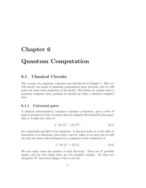
<strong>Chapter</strong> 6<br />
<strong>Quantum</strong> <strong>Computation</strong><br />
6.1 Classical Circuits<br />
The concept of a quantum computer was introduced in <strong>Chapter</strong> 1. Here we<br />
will specify our model of quantum computation more precisely, and we will<br />
point out some basic properties of the model. But before we explain what a<br />
quantum computer does, perhaps we should say what a classical computer<br />
does.<br />
6.1.1 Universal gates<br />
A classical (deterministic) computer evaluates a function: given n-bits of<br />
input it produces m-bits of output that are uniquely determined by the input;<br />
that is, it finds the value of<br />
f : {0, 1} n → {0, 1} m , (6.1)<br />
for a particular specified n-bit argument. A function with an m-bit value is<br />
equivalent to m functions, each with a one-bit value, so we may just as well<br />
say that the basic task performed by a computer is the evaluation of<br />
f : {0, 1} n → {0, 1}. (6.2)<br />
We can easily count the number of such functions. There are 2 n possible<br />
inputs, and for each input there are two possible outputs. So there are<br />
altogether 2 2n functions taking n bits to one bit.<br />
1
2 CHAPTER 6. QUANTUM COMPUTATION<br />
The evaluation of any such function can be reduced to a sequence of<br />
elementary logical operations. Let us divide the possible values of the input<br />
x = x 1 x 2 x 3 . . .x n , (6.3)<br />
into one set of values for which f(x) = 1, and a complementary set for which<br />
f(x) = 0. For each x (a) such that f(x (a) ) = 1, consider the function f (a) such<br />
that<br />
f (a) (x) =<br />
{<br />
1 x = x<br />
(a)<br />
0 otherwise<br />
(6.4)<br />
Then<br />
f(x) = f (1) (x) ∨ f (2) (x) ∨ f (3) (x) ∨ . . . . (6.5)<br />
f is the logical OR (∨) of all the f (a) ’s. In binary arithmetic the ∨ operation<br />
of two bits may be represented<br />
x ∨ y = x + y − x · y; (6.6)<br />
it has the value 0 if x and y are both zero, and the value 1 otherwise.<br />
Now consider the evaluation of f (a) . In the case where x (a) = 111. . . 1,<br />
we may write<br />
f (a) (x) = x 1 ∧ x 2 ∧ x 3 . . . ∧ x n ; (6.7)<br />
it is the logical AND (∧) of all n bits. In binary arithmetic, the AND is the<br />
product<br />
x ∧ y = x · y. (6.8)<br />
For any other x (a) , f (a) is again obtained as the AND of n bits, but where the<br />
NOT (¬) operation is first applied to each x i such that x (a)<br />
i = 0; for example<br />
if<br />
f (a) (x) = (¬x 1 ) ∧ x 2 ∧ x 3 ∧ (¬x 4 ) ∧ . . . (6.9)<br />
x (a) = 0110. . . . (6.10)
6.1. CLASSICAL CIRCUITS 3<br />
The NOT operation is represented in binary arithmetic as<br />
¬x = 1 − x. (6.11)<br />
We have now constructed the function f(x) from three elementary logical<br />
connectives: NOT, AND, OR. The expression we obtained is called the<br />
“disjunctive normal form” of f(x). We have also implicitly used another<br />
operation, COPY, that takes one bit to two bits:<br />
COPY : x → xx. (6.12)<br />
We need the COPY operation because each f (a) in the disjunctive normal<br />
form expansion of f requires its own copy of x to act on.<br />
In fact, we can pare our set of elementary logical connectives to a smaller<br />
set. Let us define a NAND (“NOT AND”) operation by<br />
x ↑ y = ¬(x ∧ y) = (¬x) ∨ (¬y). (6.13)<br />
In binary arithmetic, the NAND operation is<br />
x ↑ y = 1 − xy. (6.14)<br />
If we can COPY, we can use NAND to perform NOT:<br />
x ↑ x = 1 − x 2 = 1 − x = ¬x. (6.15)<br />
(Alternatively, if we can prepare the constant y = 1, then x ↑ 1 = 1−x = ¬x.)<br />
Also,<br />
(x ↑ y) ↑ (x ↑ y) = ¬(x ↑ y) = 1 − (1 − xy) = xy = x ∧ y,<br />
(6.16)<br />
and<br />
(x ↑ x) ↑ (y ↑ y) = (¬x) ↑ (¬y) = 1 − (1 − x)(1 − y)<br />
= x + y − xy = x ∨ y. (6.17)<br />
So if we can COPY, NAND performs AND and OR as well. We conclude<br />
that the single logical connective NAND, together with COPY, suffices to<br />
evaluate any function f. (You can check that an alternative possible choice<br />
of the universal connective is NOR:<br />
x ↓ y = ¬(x ∨ y) = (¬x) ∧ (¬y).) (6.18)
4 CHAPTER 6. QUANTUM COMPUTATION<br />
If we are able to prepare a constant bit (x = 0 or x = 1), we can reduce<br />
the number of elementary operations from two to one. The NAND/NOT<br />
gate<br />
(x, y) → (1 − x, 1 − xy), (6.19)<br />
computes NAND (if we ignore the first output bit) and performs copy (if<br />
we set the second input bit to y = 1, and we subsequently apply NOT to<br />
both output bits). We say, therefore, that NAND/NOT is a universal gate.<br />
If we have a supply of constant bits, and we can apply the NAND/NOT<br />
gates to any chosen pair of input bits, then we can perform a sequence of<br />
NAND/NOT gates to evaluate any function f : {0, 1} n → {0, 1} for any<br />
value of the input x = x 1 x 2 . . . x n .<br />
These considerations motivate the circuit model of computation. A computer<br />
has a few basic components that can perform elementary operations<br />
on bits or pairs of bits, such as COPY, NOT, AND, OR. It can also prepare<br />
a constant bit or input a variable bit. A computation is a finite sequence of<br />
such operations, a circuit, applied to a specified string of input bits. 1 The<br />
result of the computation is the final value of all remaining bits, after all the<br />
elementary operations have been executed.<br />
It is a fundamental result in the theory of computation that just a few<br />
elementary gates suffice to evaluate any function of a finite input. This<br />
result means that with very simple hardware components, we can build up<br />
arbitrarily complex computations.<br />
So far, we have only considered a computation that acts on a particular<br />
fixed input, but we may also consider families of circuits that act on inputs<br />
of variable size. Circuit families provide a useful scheme for analyzing and<br />
classifying the complexity of computations, a scheme that will have a natural<br />
generalization when we turn to quantum computation.<br />
6.1.2 Circuit complexity<br />
In the study of complexity, we will often be interested in functions with a<br />
one-bit output<br />
f : {0, 1} n → {0, 1}. (6.20)<br />
1 The circuit is required to be acyclic, meaning that no directed closed loops are<br />
permitted.
6.1. CLASSICAL CIRCUITS 5<br />
Such a function f may be said to encode a solution to a “decision problem”<br />
— the function examines the input and issues a YES or NO answer. Often, a<br />
question that would not be stated colloquially as a question with a YES/NO<br />
answer can be “repackaged” as a decision problem. For example, the function<br />
that defines the FACTORING problem is:<br />
f(x, y) =<br />
{<br />
1 if integer x has a divisor less than y,<br />
0 otherwise;<br />
(6.21)<br />
knowing f(x, y) for all y < x is equivalent to knowing the least nontrivial<br />
factor of y. Another important example of a decision problem is the HAMIL-<br />
TONIAN path problem: let the input be an l-vertex graph, represented by<br />
an l ×l adjacency matrix ( a 1 in the ij entry means there is an edge linking<br />
vertices i and j); the function is<br />
f(x) =<br />
{<br />
1 if graph x has a Hamiltonian path,<br />
0 otherwise.<br />
(6.22)<br />
(A path is Hamiltonian if it visits each vertex exactly once.)<br />
We wish to gauge how hard a problem is by quantifying the resources<br />
needed to solve the problem. For a decision problem, a reasonable measure<br />
of hardness is the size of the smallest circuit that computes the corresponding<br />
function f : {0, 1} n → {0, 1}. By size we mean the number of elementary<br />
gates or components that we must wire together to evaluate f. We may also<br />
be interested in how much time it takes to do the computation if many gates<br />
are permitted to execute in parallel. The depth of a circuit is the number of<br />
time steps required, assuming that gates acting on distinct bits can operate<br />
simultaneously (that is, the depth is the maximum length of a directed path<br />
from the input to the output of the circuit). The width of a circuit is the<br />
maximum number of gates that act in any one time step.<br />
We would like to divide the decision problems into two classes: easy and<br />
hard. But where should we draw the line? For this purpose, we consider<br />
infinite families of decision problems with variable input size; that is, where<br />
the number of bits of input can be any integer n. Then we can examine how<br />
the size of the circuit that solves the problem scales with n.<br />
If we use the scaling behavior of a circuit family to characterize the difficulty<br />
of a problem, there is a subtlety. It would be cheating to hide the<br />
difficulty of the problem in the design of the circuit. Therefore, we should
6 CHAPTER 6. QUANTUM COMPUTATION<br />
restrict attention to circuit families that have acceptable “uniformity” properties<br />
— it must be “easy” to build the circuit with n + 1 bits of input once<br />
we have constructed the circuit with an n-bit input.<br />
Associated with a family of functions {f n } (where f n has n-bit input) are<br />
circuits {C n } that compute the functions. We say that a circuit family {C n }<br />
is “polynomial size” if the size of C n grows with n no faster than a power of<br />
n,<br />
where poly denotes a polynomial. Then we define:<br />
size (C n ) ≤ poly (n), (6.23)<br />
P = {decision problem solved by polynomial-size circuit families}<br />
(P for “polynomial time”). Decision problems in P are “easy.” The rest are<br />
“hard.” Notice that C n computes f n (x) for every possible n-bit input, and<br />
therefore, if a decision problem is in P we can find the answer even for the<br />
“worst-case” input using a circuit of size no greater than poly(n). (As noted<br />
above, we implicitly assume that the circuit family is “uniform” so that the<br />
design of the circuit can itself be solved by a polynomial-time algorithm.<br />
Under this assumption, solvability in polynomial time by a circuit family is<br />
equivalent to solvability in polynomial time by a universal Turing machine.)<br />
Of course, to determine the size of a circuit that computes f n , we must<br />
know what the elementary components of the circuit are. Fortunately, though,<br />
whether a problem lies in P does not depend on what gate set we choose, as<br />
long as the gates are universal, the gate set is finite, and each gate acts on a<br />
set of bits of bounded size. One universal gate set can simulate another.<br />
The vast majority of function families f : {0, 1} n → {0, 1} are not in<br />
P. For most functions, the output is essentially random, and there is no<br />
better way to “compute” f(x) than to consult a look-up table of its values.<br />
Since there are 2 n n-bit inputs, the look-up table has exponential size, and a<br />
circuit that encodes the table must also have exponential size. The problems<br />
in P belong to a very special class — they have enough structure so that the<br />
function f can be computed efficiently.<br />
Of particular interest are decision problems that can be answered by<br />
exhibiting an example that is easy to verify. For example, given x and y < x,<br />
it is hard (in the worst case) to determine if x has a factor less than y. But<br />
if someone kindly provides a z < y that divides x, it is easy for us to check<br />
that z is indeed a factor of x. Similarly, it is hard to determine if a graph
6.1. CLASSICAL CIRCUITS 7<br />
has a Hamiltonian path, but if someone kindly provides a path, it is easy to<br />
verify that the path really is Hamiltonian.<br />
This concept that a problem may be hard to solve, but that a solution<br />
can be easily verified once found, can be formalized by the notion of a “nondeterministic”<br />
circuit. A nondeterministic circuit ˜C n,m (x (n) , y (m) ) associated<br />
with the circuit C n (x (n) ) has the property:<br />
C n (x (n) ) = 1 iff ˜C n,m (x (n) , y (m) ) = 1 for some y (m) . (6.24)<br />
(where x (n) is n bits and y (m) is m bits.) Thus for a particular x (n) we can<br />
use ˜C n,m to verify that C n (x (n) = 1, if we are fortunate enough to have the<br />
right y (m) in hand. We define:<br />
NP: {decision problems that admit a polynomial-size nondeterministic<br />
circuit family}<br />
(NP for “nondeterministic polynomial time”). If a problem is in NP, there<br />
is no guarantee that the problem is easy, only that a solution is easy to check<br />
once we have the right information. Evidently P ⊆ NP. Like P, the NP<br />
problems are a small subclass of all decision problems.<br />
Much of complexity theory is built on a fundamental conjecture:<br />
Conjecture : P ≠ NP; (6.25)<br />
there exist hard decision problems whose solutions are easily verified. Unfortunately,<br />
this important conjecture still awaits proof. But after 30 years<br />
of trying to show otherwise, most complexity experts are firmly confident of<br />
its validity.<br />
An important example of a problem in NP is CIRCUIT-SAT. In this case<br />
the input is a circuit C with n gates, m input bits, and one output bit. The<br />
problem is to find if there is any m-bit input for which the output is 1. The<br />
function to be evaluated is<br />
f(C) =<br />
{<br />
1 if there exists x (m) with C(x (m) ) = 1,<br />
0 otherwise.<br />
(6.26)<br />
This problem is in NP because, given a circuit, it is easy to simulate the<br />
circuit and evaluate its output for any particular input.<br />
I’m going to state some important results in complexity theory that will<br />
be relevant for us. There won’t be time for proofs. You can find out more
8 CHAPTER 6. QUANTUM COMPUTATION<br />
by consulting one of the many textbooks on the subject; one good one is<br />
Computers and Intractability: A Guide to the Theory of NP-Completeness,<br />
by M. R. Garey and D. S. Johnson.<br />
Many of the insights engendered by complexity theory flow from Cook’s<br />
Theorem (1971). The theorem states that every problem in NP is polynomially<br />
reducible to CIRCUIT-SAT. This means that for any PROBLEM<br />
∈ NP, there is a polynomial-size circuit family that maps an “instance” x (n)<br />
of PROBLEM to an “instance” y (m) of CIRCUIT-SAT; that is<br />
CIRCUIT − SAT (y (m) ) = 1 iff PROBLEM (x (n) ) = 1.<br />
(6.27)<br />
It follows that if we had a magical device that could efficiently solve CIRCUIT-<br />
SAT (a CIRCUIT-SAT “oracle”), we could couple that device with the polynomial<br />
reduction to efficiently solve PROBLEM. Cook’s theorem tells us that<br />
if it turns out that CIRCUIT-SAT ∈ P, then P = NP.<br />
A problem that, like CIRCUIT-SAT, has the property that every problem<br />
in NP is polynomially reducible to it, is called NP-complete (NPC).<br />
Since Cook, many other examples have been found. To show that a PROB-<br />
LEM ∈ NP is NP-complete, it suffices to find a polynomial reduction to<br />
PROBLEM of another problem that is already known to be NP-complete.<br />
For example, one can exhibit a polynomial reduction of CIRCUIT-SAT to<br />
HAMILTONIAN. It follows from Cook’s theorem that HAMILTONIAN is<br />
also NP-complete.<br />
If we assume that P ≠ NP, it follows that there exist problems in NP<br />
of intermediate difficulty (the class NPI). These are neither P nor NPC.<br />
Another important complexity class is called co-NP. Heuristically, NP<br />
decision problems are ones we can answer by exhibiting an example if the answer<br />
is YES, while co-NP problems can be answered with a counter-example<br />
if the answer is NO. More formally:<br />
{C} ∈ NP :C(x) = 1 iff C(x, y) = 1 for some y (6.28)<br />
{C} ∈ co−NP :C(x) = 1 iff C(x, y) = 1 for all y. (6.29)<br />
Clearly, there is a symmetry relating the classes NP and co-NP — whether<br />
we consider a problem to be in NP or co-NP depends on how we choose to<br />
frame the question. (“Is there a Hamiltonian circuit?” is in NP. “Is there<br />
no Hamiltonian circuit?” is in co-NP). But the interesting question is: is a<br />
problem in both NP and co-NP? If so, then we can easily verify the answer
6.1. CLASSICAL CIRCUITS 9<br />
(once a suitable example is in hand) regardless of whether the answer is YES<br />
or NO. It is believed (though not proved) that NP ≠ co−NP. (For example,<br />
we can show that a graph has a Hamiltonian path by exhibiting an example,<br />
but we don’t know how to show that it has no Hamiltonian path that way!)<br />
Assuming that NP ≠ co−NP, there is a theorem that says that no co-NP<br />
problems are contained in NPC. Therefore, problems in the intersection of<br />
NP and co-NP, if not in P, are good candidates for inclusion in NPI.<br />
In fact, a problem in NP ∩ co−NP that is believed not in P is the<br />
FACTORING problem. As already noted, FACTORING is in NP because,<br />
if we are offered a factor of x, we can easily check its validity. But it is also in<br />
co-NP, because it is known that if we are given a prime number then (at least<br />
in principle), we can efficiently verify its primality. Thus, if someone tells us<br />
the prime factors of x, we can efficiently check that the prime factorization is<br />
right, and can exclude that any integer less than y is a divisor of x. Therefore,<br />
it seems likely that FACTORING is in NPI.<br />
We are led to a crude (conjectured) picture of the structure of NP ∪<br />
co−NP. NP and co-NP do not coincide, but they have a nontrivial intersection.<br />
P lies in NP ∩ co−NP (because P = co−P), but the intersection<br />
also contains problems not in P (like FACTORING). Neither NPC nor co-<br />
NPC intersects with NP ∩ co−NP.<br />
There is much more to say about complexity theory, but we will be content<br />
to mention one more element that relates to the discussion of quantum<br />
complexity. It is sometimes useful to consider probabilistic circuits that have<br />
access to a random number generator. For example, a gate in a probabilistic<br />
circuit might act in either one of two ways, and flip a fair coin to decide which<br />
action to execute. Such a circuit, for a single fixed input, can sample many<br />
possible computational paths. An algorithm performed by a probabilistic<br />
circuit is said to be “randomized.”<br />
If we attack a decision problem using a probabilistic computer, we attain<br />
a probability distribution of outputs. Thus, we won’t necessarily always get<br />
the right answer. But if the probability of getting the right answer is larger<br />
than 1 + δ for every possible input (δ > 0), then the machine is useful. In<br />
2<br />
fact, we can run the computation many times and use majority voting to<br />
achieve an error probability less than ε. Furthermore, the number of times<br />
we need to repeat the computation is only polylogarithmic in ε −1 .<br />
If a problem admits a probabilistic circuit family of polynomial size that<br />
always gives the right answer with probability larger than 1 +δ (for any input,<br />
2<br />
and for fixed δ > 0), we say the problem is in the class BPP (“bounded-error
10 CHAPTER 6. QUANTUM COMPUTATION<br />
probabilistic polynomial time”). It is evident that<br />
P ⊆ BPP, (6.30)<br />
but the relation of NP to BPP is not known. In particular, it has not been<br />
proved that BPP is contained in NP.<br />
6.1.3 Reversible computation<br />
In devising a model of a quantum computer, we will generalize the circuit<br />
model of classical computation. But our quantum logic gates will be unitary<br />
transformations, and hence will be invertible, while classical logic gates like<br />
the NAND gate are not invertible. Before we discuss quantum circuits, it is<br />
useful to consider some features of reversible classical computation.<br />
Aside from the connection with quantum computation, another incentive<br />
for studying reversible classical computation arose in <strong>Chapter</strong> 1. As Landauer<br />
observed, because irreversible logic elements erase information, they<br />
are necessarily dissipative, and therefore, require an irreducible expenditure<br />
of power. But if a computer operates reversibly, then in principle there need<br />
be no dissipation and no power requirement. We can compute for free!<br />
A reversible computer evaluates an invertible function taking n bits to n<br />
bits<br />
f : {0, 1} n → {0, 1} n , (6.31)<br />
the function must be invertible so that there is a unique input for each output;<br />
then we are able in principle to run the computation backwards and recover<br />
the input from the output. Since it is a 1-1 function, we can regard it as a<br />
permutation of the 2 n strings of n bits — there are (2 n )! such functions.<br />
Of course, any irreversible computation can be “packaged” as an evaluation<br />
of an invertible function. For example, for any f : {0, 1} n → {0, 1} m ,<br />
we can construct ˜f : {0, 1} n+m → {0, 1} n+m such that<br />
˜f(x; 0 (m) ) = (x; f(x)), (6.32)<br />
(where 0 (m) denotes m-bits initially set to zero). Since ˜f takes each (x; 0 (m) )<br />
to a distinct output, it can be extended to an invertible function of n + m<br />
bits. So for any f taking n bits to m, there is an invertible ˜f taking n + m<br />
to n + m, which evaluates f(x) acting on (x, 0 (m) )
6.1. CLASSICAL CIRCUITS 11<br />
Now, how do we build up a complicated reversible computation from<br />
elementary components — that is, what constitutes a universal gate set? We<br />
will see that one-bit and two-bit reversible gates do not suffice; we will need<br />
three-bit gates for universal reversible computation.<br />
Of the four 1-bit → 1-bit gates, two are reversible; the trivial gate and<br />
the NOT gate. Of the (2 4 ) 2 = 256 possible 2-bit → 2-bit gates, 4! = 24 are<br />
reversible. One of special interest is the controlled-NOT or reversible XOR<br />
gate that we already encountered in <strong>Chapter</strong> 4:<br />
XOR : (x, y) ↦→ (x, x ⊕ y), (6.33)<br />
x<br />
y<br />
<br />
❣<br />
x<br />
x ⊕ y<br />
This gate flips the second bit if the first is 1, and does nothing if the first bit<br />
is 0 (hence the name controlled-NOT). Its square is trivial, that is, it inverts<br />
itself. Of course, this gate performs a NOT on the second bit if the first bit<br />
is set to 1, and it performs the copy operation if y is initially set to zero:<br />
With the circuit<br />
XOR : (x, 0) ↦→ (x, x). (6.34)<br />
x<br />
<br />
❣<br />
<br />
y<br />
y<br />
❣<br />
<br />
❣<br />
x<br />
constructed from three X0R’s, we can swap two bits:<br />
(x, y) → (x, x ⊕ y) → (y, x ⊕ y) → (y, x). (6.35)<br />
With these swaps we can shuffle bits around in a circuit, bringing them<br />
together if we want to act on them with a particular component in a fixed<br />
location.<br />
To see that the one-bit and two-bit gates are nonuniversal, we observe<br />
that all these gates are linear. Each reversible two-bit gate has an action of<br />
the form<br />
( ) ( ) ( )<br />
x x<br />
′<br />
( ) x a<br />
→ = M + , (6.36)<br />
y y ′ y b
12 CHAPTER 6. QUANTUM COMPUTATION<br />
where the constant ( )<br />
a<br />
b takes one of four possible values, and the matrix M<br />
is one of the six invertible matrices<br />
( ) ( ) ( ) ( ) ( ) ( )<br />
1 0 0 1 1 1 1 0 0 1 1 1<br />
M = , , , , , .<br />
0 1 1 0 0 1 1 1 1 1 1 0<br />
(6.37)<br />
(All addition is performed modulo 2.) Combining the six choices for M with<br />
the four possible constants, we obtain 24 distinct gates, which exhausts all<br />
the reversible 2 → 2 gates.<br />
Since the linear transformations are closed under composition, any circuit<br />
composed from reversible 2 → 2 (and 1 → 1) gates will compute a linear<br />
function<br />
x → Mx + a. (6.38)<br />
But for n ≥ 3, there are invertible functions on n-bits that are nonlinear. An<br />
important example is the 3-bit Toffoli gate (or controlled-controlled-NOT)<br />
θ (3) θ (3) : (x, y, z) → (x, y, z ⊕ xy); (6.39)<br />
x<br />
y<br />
z<br />
<br />
<br />
❣<br />
x<br />
y<br />
z ⊕ xy<br />
it flips the third bit if the first two are 1 and does nothing otherwise. Like<br />
the XOR gate, it is its own inverse.<br />
Unlike the reversible 2-bit gates, the Toffoli gate serves as a universal gate<br />
for Boolean logic, if we can provide fixed input bits and ignore output bits.<br />
If z is initially 1, then x ↑ y = 1 − xy appears in the third output — we can<br />
perform NAND. If we fix x = 1, the Toffoli gate functions like an XOR gate,<br />
and we can use it to copy.<br />
The Toffoli gate θ (3) is universal in the sense that we can build a circuit to<br />
compute any reversible function using Toffoli gates alone (if we can fix input<br />
bits and ignore output bits). It will be instructive to show this directly,<br />
without relying on our earlier argument that NAND/NOT is universal for<br />
Boolean functions. In fact, we can show the following: From the NOT gate
6.1. CLASSICAL CIRCUITS 13<br />
and the Toffoli gate θ (3) , we can construct any invertible function on n bits,<br />
provided we have one extra bit of scratchpad space available.<br />
The first step is to show that from the three-bit Toffoli-gate θ (3) we can<br />
construct an n-bit Toffoli gate θ (n) that acts as<br />
(x 1 , x 2 , . . . x n−1 , y) → (x 1 , x 2 , . . . , x n−1 y ⊕ x 1 x 2 . . . x n−1 ).<br />
(6.40)<br />
The construction requires one extra bit of scratch space. For example, we<br />
construct θ (4) from θ (3) ’s with the circuit<br />
x 1<br />
<br />
<br />
x 1<br />
x 2<br />
<br />
<br />
x 2<br />
0<br />
❣ <br />
❣<br />
0<br />
x 3<br />
<br />
x 3<br />
y<br />
❣<br />
y ⊕ x 1 x 2 x 3<br />
The purpose of the last θ (3) gate is to reset the scratch bit back to its original<br />
value zero. Actually, with one more gate we can obtain an implementation<br />
of θ (4) that works irrespective of the initial value of the scratch bit:<br />
x 1<br />
<br />
<br />
x 1<br />
x 2<br />
<br />
<br />
x 2<br />
w<br />
❣ <br />
❣ <br />
w<br />
x 3<br />
<br />
<br />
x 3<br />
y<br />
❣<br />
❣<br />
y ⊕ x 1 x 2 x 3<br />
Again, we can eliminate the last gate if we don’t mind flipping the value of<br />
the scratch bit.<br />
We can see that the scratch bit really is necessary, because θ (4) is an odd<br />
permutation (in fact a transposition) of the 24 4-bit strings — it transposes<br />
1111 and 1110. But θ (3) acting on any three of the four bits is an even<br />
permutation; e.g., acting on the last three bits it transposes 0111 with 0110,
14 CHAPTER 6. QUANTUM COMPUTATION<br />
and 1111 with 1110. Since a product of even permutations is also even, we<br />
cannot obtain θ (4) as a product of θ (3) ’s that act on four bits only.<br />
The construction of θ (4) from four θ (3) ’s generalizes immediately to the<br />
construction of θ (n) from two θ (n−1) ’s and two θ (3) ’s (just expand x 1 to several<br />
control bits in the above diagram). Iterating the construction, we obtain θ (n)<br />
from a circuit with 2 n−2 +2 n−3 −2 θ (3) ’s. Furthermore, just one bit of scratch<br />
space is sufficient. 2 ) (When we need to construct θ (k) , any available extra<br />
bit will do, since the circuit returns the scratch bit to its original value. The<br />
next step is to note that, by conjugating θ (n) with NOT gates, we can in<br />
effect modify the value of the control string that “triggers” the gate. For<br />
example, the circuit<br />
x 1<br />
❣<br />
<br />
❣<br />
x 2<br />
<br />
x 3<br />
❣<br />
<br />
❣<br />
y<br />
❣<br />
flips the value of y if x 1 x 2 x 3 = 010, and it acts trivially otherwise. Thus<br />
this circuit transposes the two strings 0100 and 0101. In like fashion, with<br />
θ (n) and NOT gates, we can devise a circuit that transposes any two n-bit<br />
strings that differ in only one bit. (The location of the bit where they differ<br />
is chosen to be the target of the θ (n) gate.)<br />
But in fact a transposition that exchanges any two n-bit strings can be<br />
expressed as a product of transpositions that interchange strings that differ<br />
in only one bit. If a 0 and a s are two strings that are Hamming distance s<br />
apart (differ in s places), then there is a chain<br />
a 0 , a 1 , a 2 , a 3 , . . . , a s , (6.41)<br />
such that each string in the chain is Hamming distance one from its neighbors.<br />
Therefore, each of the transpositions<br />
(a 0 a 1 ), (a 1 a 2 ), (a 2 a 3 ), . . .(a s−1 a s ), (6.42)<br />
2 With more scratch space, we can build θ (n) from θ (3) ’s much more efficiently — see<br />
the exercises.
6.1. CLASSICAL CIRCUITS 15<br />
can be implemented as a θ (n) gate conjugated by NOT gates. By composing<br />
transpositions we find<br />
(a 0 a s ) = (a s−1 a s )(a s−2 a s−1 )...(a 2 a 3 )(a 1 a 2 )(a 0 a 1 )(a 1 a 2 )(a 2 a 3 )<br />
. . .(a s−2 a s−1 )(a s−1 a s ); (6.43)<br />
we can construct the Hamming-distance-s transposition from 2s−1 Hammingdistance-one<br />
transpositions. It follows that we can construct (a 0 a s ) from<br />
θ (n) ’s and NOT gates.<br />
Finally, since every permutation is a product of transpositions, we have<br />
shown that every invertible function on n-bits (every permutation on n-bit<br />
strings) is a product of θ (3) ’s and NOT’s, using just one bit of scratch space.<br />
Of course, a NOT can be performed with a θ (3) gate if we fix two input<br />
bits at 1. Thus the Toffoli gate θ (3) is universal for reversible computation,<br />
if we can fix input bits and discard output bits.<br />
6.1.4 Billiard ball computer<br />
Two-bit gates suffice for universal irreversible computation, but three-bit<br />
gates are needed for universal reversible computation. One is tempted to<br />
remark that “three-body interactions” are needed, so that building reversible<br />
hardware is more challenging than building irreversible hardware. However,<br />
this statement may be somewhat misleading.<br />
Fredkin described how to devise a universal reversible computer in which<br />
the fundamental interaction is an elastic collision between two billiard balls.<br />
1<br />
Balls of radius √<br />
2<br />
move on a square lattice with unit lattice spacing. At<br />
each integer valued time, the center of each ball lies at a lattice site; the<br />
presence or absence of a ball at a particular site (at integer time) encodes<br />
a bit of information. In each unit of time, each ball moves unit distance<br />
along one of the lattice directions. Occasionally, at integer-valued times, 90 o<br />
elastic √ collisions occur between two balls that occupy sites that are distance<br />
2 apart (joined by a lattice diagonal).<br />
The device is programmed by nailing down balls at certain sites, so that<br />
those balls act as perfect reflectors. The program is executed by fixing initial<br />
positions and directions for the moving balls, and evolving the system<br />
according to Newtonian mechanics for a finite time. We read the output<br />
by observing the final positions of all the moving balls. The collisions are<br />
nondissipative, so that we can run the computation backward by reversing<br />
the velocities of all the balls.
16 CHAPTER 6. QUANTUM COMPUTATION<br />
To show that this machine is a universal reversible computer, we must<br />
explain how to operate a universal gate. It is convenient to consider the<br />
three-bit Fredkin gate<br />
(x, y, z) → (x, xz + ¯xy, xy + ¯xz), (6.44)<br />
which swaps y and z if x = 0 (we have introduced the notation ¯x = ¬x).<br />
You can check that the Fredkin gate can simulate a NAND/NOT gate if we<br />
fix inputs and ignore outputs.<br />
We can build the Fredkin gate from a more primitive object, the switch<br />
gate. A switch gate taking two bits to three acts as<br />
(x, y) → (x, xy, ¯xy). (6.45)<br />
x<br />
y<br />
S<br />
x<br />
xy<br />
¯xy<br />
The gate is “reversible” in that we can run it backwards acting on a constrained<br />
3-bit input taking one of the four values<br />
⎛ ⎞ ⎛ ⎞ ⎛ ⎞ ⎛ ⎞ ⎛ ⎞<br />
x 0 0 1 1<br />
⎜ ⎟ ⎜ ⎟ ⎜ ⎟ ⎜ ⎟ ⎜ ⎟<br />
⎝ y ⎠ = ⎝ 0 ⎠ ⎝ 0 ⎠ ⎝ 0 ⎠ ⎝ 1 ⎠ (6.46)<br />
z 0 1 0 0<br />
Furthermore, the switch gate is itself universal; fixing inputs and ignoring<br />
outputs, it can do NOT (y = 1, third output) AND (second output), and<br />
COPY (y = 1, first and second output). It is not surprising, then, that we<br />
can compose switch gates to construct a universal reversible 3 → 3 gate.<br />
Indeed, the circuit<br />
builds the Fredkin gate from four switch gates (two running forward and two<br />
running backward). Time delays needed to maintain synchronization are not<br />
explicitly shown.<br />
In the billiard ball computer, the switch gate is constructed with two<br />
reflectors, such that (in the case x = y = 1) two moving balls collide twice.<br />
The trajectories of the balls in this case are:
6.1. CLASSICAL CIRCUITS 17<br />
A ball labeled x emerges from the gate along the same trajectory (and at the<br />
same time) regardless of whether the other ball is present. But for x = 1, the<br />
position of the other ball (if present) is shifted down compared to its final<br />
position for x = 0 — this is a switch gate. Since we can perform a switch<br />
gate, we can construct a Fredkin gate, and implement universal reversible<br />
logic with a billiard ball computer.<br />
An evident weakness of the billiard-ball scheme is that initial errors in the<br />
positions and velocities of the ball will accumulate rapidly, and the computer<br />
will eventually fail. As we noted in <strong>Chapter</strong> 1 (and Landauer has insistently<br />
pointed out) a similar problem will afflict any proposed scheme for dissipationless<br />
computation. To control errors we must be able to compress the<br />
phase space of the device, which will necessarily be a dissipative process.<br />
6.1.5 Saving space<br />
But even aside from the issue of error control there is another key question<br />
about reversible computation. How do we manage the scratchpad space<br />
needed to compute reversibly?<br />
In our discussion of the universality of the Toffoli gate, we saw that in<br />
principle we can do any reversible computation with very little scratch space.<br />
But in practice it may be impossibly difficult to figure out how to do a<br />
particular computation with minimal space, and in any case economizing on<br />
space may be costly in terms of the run time.<br />
There is a general strategy for simulating an irreversible computation on<br />
a reversible computer. Each irreversible NAND or COPY gate can be simulated<br />
by a Toffoli gate by fixing inputs and ignoring outputs. We accumulate<br />
and save all “garbage” output bits that are needed to reverse the steps of<br />
the computation. The computation proceeds to completion, and then a copy<br />
of the output is generated. (This COPY operation is logically reversible.)<br />
Then the computation runs in reverse, cleaning up all garbage bits, and returning<br />
all registers to their original configurations. With this procedure<br />
the reversible circuit runs only about twice as long as the irreversible circuit<br />
that it simulates, and all garbage generated in the simulation is disposed of<br />
without any dissipation and hence no power requirement.<br />
This procedure works, but demands a huge amount of scratch space – the<br />
space needed scales linearly with the length T of the irreversible computation<br />
being simulated. In fact, it is possible to use space far more efficiently (with<br />
only a minor slowdown), so that the space required scales like log T instead
18 CHAPTER 6. QUANTUM COMPUTATION<br />
of T. (That is, there is a general-purpose scheme that requires space ∝<br />
log T; of course, we might do even better in the simulation of a particular<br />
computation.)<br />
To use space more effectively, we will divide the computation into smaller<br />
steps of roughly equal size, and we will run these steps backward when possible<br />
during the course of the computation. However, just as we are unable<br />
to perform step k of the computation unless step k − 1 has already been<br />
completed, we are unable to run step k in reverse if step k −1 has previously<br />
been executed in reverse. 3 The amount of space we require (to store our<br />
garbage) will scale like the maximum value of the number of forward steps<br />
minus the number of backward steps that have been executed.<br />
The challenge we face can be likened to a game — the reversible pebble<br />
game. 4 The steps to be executed form a one-dimension directed graph with<br />
sites labeled 1, 2, 3. . . T. Execution of step k is modeled by placing a pebble<br />
on the kth site of the graph, and executing step k in reverse is modeled as<br />
removal of a pebble from site k. At the beginning of the game, no sites are<br />
covered by pebbles, and in each turn we add or remove a pebble. But we<br />
cannot place a pebble at site k (except for k = 1) unless site k − 1 is already<br />
covered by a pebble, and we cannot remove a pebble from site k (except for<br />
k = 1) unless site k − 1 is covered. The object is to cover site T (complete<br />
the computation) without using more pebbles than necessary (generating a<br />
minimal amount of garbage).<br />
In fact, with n pebbles we can reach site T = 2 n − 1, but we can go no<br />
further.<br />
We can construct a recursive procedure that enables us to reach site<br />
T = 2 n−1 with n pebbles, leaving only one pebble in play. Let F 1 (k) denote<br />
placing a pebble at site k, and F 1 (k) −1 denote removing a pebble from site<br />
k. Then<br />
F 2 (1, 2) = F 1 (1)F 1 (2)F 1 (1) −1 , (6.47)<br />
leaves a pebble at site k = 2, using a maximum of two pebbles at intermediate<br />
3 We make the conservative assumption that we are not clever enough to know ahead<br />
of time what portion of the output from step k − 1 might be needed later on. So we store<br />
a complete record of the configuration of the machine after step k − 1, which is not to be<br />
erased until an updated record has been stored after the completion of a subsequent step.<br />
4 as pointed out by Bennett. For a recent discussion, see M. Li and P. Vitanyi,<br />
quant-ph/9703022.
6.1. CLASSICAL CIRCUITS 19<br />
stages. Similarly<br />
F 3 (1, 4) = F 2 (1, 2)F 2 (3, 4)F 2 (1, 2) −1 , (6.48)<br />
reaches site k = 4 using a maximum of three pebbles, and<br />
F 4 (1, 8) = F 3 (1, 4)F 3 (5, 8)F 3 (1, 4) −1 , (6.49)<br />
reaches k = 8 using four pebbles. Evidently we can construct F n (1, 2 n−1 )<br />
which uses a maximum of n pebbles and leaves a single pebble in play. (The<br />
routine<br />
F n (1, 2 n−1 )F n−1 (2 n−1 + 1, 2 n−1 + 2 n−2 )...F 1 (2 n − 1),<br />
(6.50)<br />
leaves all n pebbles in play, with the maximal pebble at site k = 2 n − 1.)<br />
Interpreted as a routine for executing T = 2 n−1 steps of a computation,<br />
this strategy for playing the pebble game represents a simulation requiring<br />
space scaling like n ∼ log T. How long does the simulation take? At each level<br />
of the recursive procedure described above, two steps forward are replaced by<br />
two steps forward and one step back. Therefore, an irreversible computation<br />
with T irr = 2 n steps is simulated in T rev = 3 n steps, or<br />
a modest power law slowdown.<br />
In fact, we can improve the slowdown to<br />
T rev = (T irr ) log3/log 2 , = (T irr ) 1.58 , (6.51)<br />
T rev ∼ (T irr ) 1+ε , (6.52)<br />
for any ε > 0. Instead of replacing two steps forward with two forward and<br />
one back, we replace l forward with l forward and l − 1 back. A recursive<br />
procedure with n levels reaches site l n using a maximum of n(l − 1) + 1<br />
pebbles. Now we have T irr = l n and T rev = (2l − 1) n , so that<br />
T rev = (T irr ) log(2l−1)/log l ; (6.53)<br />
the power characterizing the slowdown is<br />
log(2l − 1)<br />
log l<br />
= log 2l + log ( 1 − 1 2l<br />
log l<br />
)<br />
≃ 1 + log 2<br />
log l , (6.54)
20 CHAPTER 6. QUANTUM COMPUTATION<br />
and the space requirement scales as<br />
S ≃ nl ≃ l log T<br />
log l . (6.55)<br />
Thus, for any fixed ε > 0, we can attain S scaling like log T, and a slowdown<br />
no worse than (T irr ) 1+ε . (This is not the optimal way to play the Pebble game<br />
if our objective is to get as far as we can with as few pebbles as possible. We<br />
use more pebbles to get to step T, but we get there faster.)<br />
We have now seen that a reversible circuit can simulate a circuit composed<br />
of irreversible gates efficiently — without requiring unreasonable memory<br />
resources or causing an unreasonable slowdown. Why is this important?<br />
You might worry that, because reversible computation is “harder” than irreversible<br />
computation, the classification of complexity depends on whether<br />
we compute reversibly or irreversibly. But this is not the case, because a<br />
reversible computer can simulate an irreversible computer pretty easily.<br />
6.2 <strong>Quantum</strong> Circuits<br />
Now we are ready to formulate a mathematical model of a quantum computer.<br />
We will generalize the circuit model of classical computation to the<br />
quantum circuit model of quantum computation.<br />
A classical computer processes bits. It is equipped with a finite set of<br />
gates that can be applied to sets of bits. A quantum computer processes<br />
qubits. We will assume that it too is equipped with a discrete set of fundamental<br />
components, called quantum gates. Each quantum gate is a unitary<br />
transformation that acts on a fixed number of qubits. In a quantum computation,<br />
a finite number n of qubits are initially set to the value |00. . . 0〉.<br />
A circuit is executed that is constructed from a finite number of quantum<br />
gates acting on these qubits. Finally, a Von Neumann measurement of all the<br />
qubits (or a subset of the qubits) is performed, projecting each onto the basis<br />
{|0〉, |1〉}. The outcome of this measurement is the result of the computation.<br />
Several features of this model require comment:<br />
(1) It is implicit but important that the Hilbert space of the device has a preferred<br />
decomposition into a tensor product of low-dimensional spaces,<br />
in this case the two-dimensional spaces of the qubits. Of course, we<br />
could have considered a tensor product of, say, qutrits instead. But
6.2. QUANTUM CIRCUITS 21<br />
anyway we assume there is a natural decomposition into subsystems<br />
that is respected by the quantum gates — which act on only a few<br />
subsystems at a time. Mathematically, this feature of the gates is crucial<br />
for establishing a clearly defined notion of quantum complexity.<br />
Physically, the fundamental reason for a natural decomposition into<br />
subsystems is locality; feasible quantum gates must act in a bounded<br />
spatial region, so the computer decomposes into subsystems that interact<br />
only with their neighbors.<br />
(2) Since unitary transformations form a continuum, it may seem unnecessarily<br />
restrictive to postulate that the machine can execute only those<br />
quantum gates chosen from a discrete set. We nevertheless accept such<br />
a restriction, because we do not want to invent a new physical implementation<br />
each time we are faced with a new computation to perform.<br />
(3) We might have allowed our quantum gates to be superoperators, and our<br />
final measurement to be a POVM. But since we can easily simulate a<br />
superoperator by performing a unitary transformation on an extended<br />
system, or a POVM by performing a Von Neumann measurement on<br />
an extended system, the model as formulated is of sufficient generality.<br />
(4) We might allow the final measurement to be a collective measurement,<br />
or a projection into a different basis. But any such measurement can be<br />
implemented by performing a suitable unitary transformation followed<br />
by a projection onto the standard basis {|0〉, |1〉} n . Of course, complicated<br />
collective measurements can be transformed into measurements<br />
in the standard basis only with some difficulty, but it is appropriate to<br />
take into account this difficulty when characterizing the complexity of<br />
an algorithm.<br />
(5) We might have allowed measurements at intermediate stages of the<br />
computation, with the subsequent choice of quantum gates conditioned<br />
on the outcome of those measurements. But in fact the same result<br />
can always be achieved by a quantum circuit with all measurements<br />
postponed until the end. (While we can postpone the measurements in<br />
principle, it might be very useful in practice to perform measurements<br />
at intermediate stages of a quantum algorithm.)<br />
A quantum gate, being a unitary transformation, is reversible. In fact, a<br />
classical reversible computer is a special case of a quantum computer. A
22 CHAPTER 6. QUANTUM COMPUTATION<br />
classical reversible gate<br />
x (n) → y (n) = f(x (n) ), (6.56)<br />
implementing a permutation of n-bit strings, can be regarded as a unitary<br />
transformation that acts on the “computational basis {|x i 〉} according to<br />
U : |x i 〉 → |y i 〉. (6.57)<br />
This action is unitary because the 2 n strings |y i 〉 are all mutually orthogonal.<br />
A quantum computation constructed from such classical gates takes |0. . . 0〉<br />
to one of the computational basis states, so that the final measurement is<br />
deterministic.<br />
There are three main issues concerning our model that we would like to<br />
address. The first issue is universality. The most general unitary transformation<br />
that can be performed on n qubits is an element of U(2 n ). Our model<br />
would seem incomplete if there were transformations in U(2 n ) that we were<br />
unable to reach. In fact, we will see that there are many ways to choose a<br />
discrete set of universal quantum gates. Using a universal gate set we can<br />
construct circuits that compute a unitary transformation that comes as close<br />
as we please to any element in U(2 n ).<br />
Thanks to universality, there is also a machine independent notion of<br />
quantum complexity. We may define a new complexity class BQP — the class<br />
of decision problems that can be solved, with high probability, by polynomialsize<br />
quantum circuits. Since one universal quantum computer can simulate<br />
another efficiently, the class does not depend on the details of our hardware<br />
(on the universal gate set that we have chosen).<br />
Notice that a quantum computer can easily simulate a probabilistic classical<br />
computer: it can prepare √ 1<br />
2<br />
(|0〉 + |1〉) and then project to {|0〉, |1〉},<br />
generating a random bit. Therefore BQP certainly contains the class BPP.<br />
But as we discussed in <strong>Chapter</strong> 1, it seems to be quite reasonable to expect<br />
that BQP is actually larger than BPP, because a probabilistic classical<br />
computer cannot easily simulate a quantum computer. The fundamental difficulty<br />
is that the Hilbert space of n qubits is huge, of dimension 2 n , and<br />
hence the mathematical description of a typical vector in the space is exceedingly<br />
complex. Our second issue is to better characterize the resources<br />
needed to simulate a quantum computer on a classical computer. We will see<br />
that, despite the vastness of Hilbert space, a classical computer can simulate<br />
an n-qubit quantum computer even if limited to an amount of memory space
6.2. QUANTUM CIRCUITS 23<br />
that is polynomial in n. This means the BQP is contained in the complexity<br />
class PSPACE, the decision problems that can be solved with polynomial<br />
space, but may require exponential time. (We know that NP is also contained<br />
in PSPACE, since checking if C(x (n) , y (m) ) = 1 for each y (m) can be<br />
accomplished with polynomial space. 5<br />
The third important issue we should address is accuracy. The class BQP<br />
is defined formally under the idealized assumption that quantum gates can be<br />
executed with perfect precision. Clearly, it is crucial to relax this assumption<br />
in any realistic implementation of quantum computation. A polynomial size<br />
quantum circuit family that solves a hard problem would not be of much<br />
interest if the quantum gates in the circuit were required to have exponential<br />
accuracy. In fact, we will show that this is not the case. An idealized T-gate<br />
quantum circuit can be simulated with acceptable accuracy by noisy gates,<br />
provided that the error probability per gate scales like 1/T.<br />
We see that quantum computers pose a serious challenge to the strong<br />
Church–Turing thesis, which contends that any physically reasonable model<br />
of computation can be simulated by probabilistic classical circuits with at<br />
worst a polynomial slowdown. But so far there is no firm proof that<br />
BPP ≠ BQP. (6.58)<br />
Nor is such a proof necessarily soon to be expected. 6<br />
would be<br />
Indeed, a corollary<br />
BPP ≠ PSPACE, (6.59)<br />
which would settle one of the long-standing and pivotal open questions in<br />
complexity theory.<br />
It might be less unrealistic to hope for a proof that BPP ≠ BQP follows<br />
from another standard conjecture of complexity theory such as P ≠ NP. So<br />
far no such proof has been found. But while we are not yet able to prove<br />
that quantum computers have capabilities far beyond those of conventional<br />
computers, we nevertheless might uncover evidence suggesting that BPP ≠<br />
BQP. We will see that there are problems that seem to be hard (in classical<br />
computation) yet can be efficiently solved by quantum circuits.<br />
5 Actually there is another rung of the complexity hierarchy that may separate BQP<br />
and PSPACE; we can show that BQP ⊆ P #P ⊆ PSPACE, but we won’t consider P #P<br />
any further here.<br />
6 That is, we ought not to expect a “nonrelativized proof.” A separation between BPP<br />
and BQP “relative to an oracle” will be established later in the chapter.
24 CHAPTER 6. QUANTUM COMPUTATION<br />
Thus it seems likely that the classification of complexity will be different<br />
depending on whether we use a classical computer or a quantum computer<br />
to solve a problem. If such a separation really holds, it is the quantum<br />
classification that should be regarded as the more fundamental, for it is<br />
better founded on the physical laws that govern the universe.<br />
6.2.1 Accuracy<br />
Let’s discuss the issue of accuracy. We imagine that we wish to implement<br />
a computation in which the quantum gates U 1 , U 2 , . . . , U T are applied sequentially<br />
to the initial state |ϕ 0 〉. The state prepared by our ideal quantum<br />
circuit is<br />
|ϕ T 〉 = U T U T −1 . . . U 2 U 1 |ϕ 0 〉. (6.60)<br />
But in fact our gates do not have perfect accuracy. When we attempt to apply<br />
the unitary transformation U t , we instead apply some “nearby” unitary<br />
transformation Ũt. (Of course, this is not the most general type of error that<br />
we might contemplate – the unitary U t might be replaced by a superoperator.<br />
Considerations similar to those below would apply in that case, but for now<br />
we confine our attention to “unitary errors.”)<br />
The errors cause the actual state of the computer to wander away from<br />
the ideal state. How far does it wander? Let |ϕ t 〉 denote the ideal state after<br />
t quantum gates are applied, so that<br />
But if we apply the actual transformation Ũ t , then<br />
where<br />
|ϕ t 〉 = U t |ϕ t−1 〉. (6.61)<br />
Ũ t |ϕ t−1 〉 = |ϕ t 〉 + |E t 〉, (6.62)<br />
|E t 〉 = (Ũt − U t )|ϕ t−1 〉, (6.63)<br />
is an unnormalized vector. If | ˜ϕ t 〉 denotes the actual state after t steps, then<br />
we have<br />
| ˜ϕ 1 〉 = |ϕ 1 〉 + |E 1 〉,<br />
| ˜ϕ 2 〉 = Ũ 2| ˜ϕ 1 〉 = |ϕ 2 〉 + |E 2 〉 + Ũ 2|E 1 〉, (6.64)
6.2. QUANTUM CIRCUITS 25<br />
and so forth; we ultimately obtain<br />
| ˜ϕ T 〉 = |ϕ T 〉 + |E T 〉 + ŨT |E T −1 〉 + Ũ TŨT −1|E T −2 〉<br />
+ . . . + Ũ TŨT −1 . . .Ũ 2|E 1 〉. (6.65)<br />
Thus we have expressed the difference between | ˜ϕ T 〉 and |ϕ T 〉 as a sum of T<br />
remainder terms. The worst case yielding the largest deviation of | ˜ϕ T 〉 from<br />
|ϕ T 〉 occurs if all remainder terms line up in the same direction, so that the<br />
errors interfere constructively. Therefore, we conclude that<br />
‖ | ˜ϕ T 〉 − |ϕ T 〉 ‖ ≤<br />
‖ |E T 〉 ‖ + ‖ |E T −1 〉 ‖<br />
+ . . . + ‖ |E 2 〉 ‖ + ‖ |E 1 〉 ‖, (6.66)<br />
where we have used the property ‖ U|E i 〉 ‖=‖ |E i 〉 ‖ for any unitary U.<br />
Let ‖ A ‖ sup denote the sup norm of the operator A — that is, the<br />
maximum modulus of an eigenvalue of A. We then have<br />
‖ |E t 〉 ‖=‖ ( Ũ t − U t<br />
)<br />
|ϕt−1 〉 ‖≤‖ Ũt − U t ‖ sup (6.67)<br />
(since |ϕ t−1 〉 is normalized). Now suppose that, for each value of t, the error<br />
in our quantum gate is bounded by<br />
Then after T quantum gates are applied, we have<br />
‖ Ũ t − U t ‖ sup < ε. (6.68)<br />
‖ | ˜ϕ T 〉 − |ϕ T 〉 ‖< Tε; (6.69)<br />
in this sense, the accumulated error in the state grows linearly with the length<br />
of the computation.<br />
The distance bounded in eq. (6.68) can equivalently be expressed as ‖<br />
W t −1 ‖ sup , where W t = ŨtU † t. Since W t is unitary, each of its eigenvalues<br />
is a phase e iθ , and the corresponding eigenvalue of W t − 1 has modulus<br />
|e iθ − 1| = (2 − 2cos θ) 1/2 , (6.70)<br />
so that eq. (6.68) is the requirement that each eigenvalue satisfies<br />
cos θ > 1 − ε 2 /2, (6.71)
26 CHAPTER 6. QUANTUM COMPUTATION<br />
(or |θ| ∼ < ε, for ε small). The origin of eq. (6.69) is clear. In each time step,<br />
| ˜ϕ〉 rotates relative to |ϕ〉 by (at worst) an angle of order ε, and the distance<br />
between the vectors increases by at most of order ε.<br />
How much accuracy is good enough? In the final step of our computation,<br />
we perform an orthogonal measurement, and the probability of outcome a,<br />
in the ideal case, is<br />
Because of the errors, the actual probability is<br />
P(a) = |〈a|ϕ T 〉| 2 . (6.72)<br />
˜P(a) = |〈a| ˜ϕ T 〉| 2 . (6.73)<br />
If the actual vector is close to the ideal vector, then the probability distributions<br />
are close, too. If we sum over an orthonormal basis {|a〉}, we have<br />
∑<br />
| ˜P(a) − P(a)| ≤ 2 ‖ | ˜ϕ T 〉 − |ϕ T 〉 ‖, (6.74)<br />
a<br />
as you will show in a homework exercise. Therefore, if we keep Tε fixed (and<br />
small) as T gets large, the error in the probability distribution also remains<br />
fixed. In particular, if we have designed a quantum algorithm that solves a<br />
decision problem correctly with probability greater 1 + δ (in the ideal case),<br />
2<br />
then we can achieve success probability greater than 1 with our noisy gates,<br />
2<br />
if we can perform the gates with an accuracy Tε < O(δ). A quantum circuit<br />
family in the BQP class can really solve hard problems, as long as we can<br />
improve the accuracy of the gates linearly with the computation size T.<br />
6.2.2 BQP ⊆ PSPACE<br />
Of course a classical computer can simulate any quantum circuit. But how<br />
much memory does the classical computer require? Naively, since the simulation<br />
of an n-qubit circuit involves manipulating matrices of size 2 n , it may<br />
seem that an amount of memory space exponential in n is needed. But we<br />
will now show that the simulation can be done to acceptable accuracy (albeit<br />
very slowly!) in polynomial space. This means that the quantum complexity<br />
class BQP is contained in the class PSPACE of problems that can be solved<br />
with polynomial space.<br />
The object of the classical simulation is to compute the probability for<br />
each possible outcome a of the final measurement<br />
Prob(a) = |〈a|U T |0〉| 2 , (6.75)
6.2. QUANTUM CIRCUITS 27<br />
where<br />
U T = U T U T −1 . . . U 2 U 1 , (6.76)<br />
is a product of T quantum gates. Each U t , acting on the n qubits, can be<br />
represented by a 2 n ×2 n unitary matrix, characterized by the complex matrix<br />
elements<br />
〈y|U t |x〉, (6.77)<br />
where x, y ∈ {0, 1. . . , 2 n − 1}. Writing out the matrix multiplication explicitly,<br />
we have<br />
〈a|U T |0〉 = ∑ {x t}〈a|U T |x T −1 〉〈x T −1 |U T −1 |x T −2 〉. . .<br />
. . . 〈x 2 |U 2 |x 1 〉〈x 1 |U 1 |0〉. (6.78)<br />
Eq. (6.78) is a sort of “path integral” representation of the quantum computation<br />
– the probability amplitude for the final outcome a is expressed as a<br />
coherent sum of amplitudes for each of a vast number (2 n(T −1) ) of possible<br />
computational paths that begin at 0 and terminate at a after T steps.<br />
Our classical simulator is to add up the 2 n(T −1) complex numbers in<br />
eq. (6.78) to compute 〈a|U T |0〉. The first problem we face is that finite size<br />
classical circuits do integer arithmetic, while the matrix elements 〈y|U t |x〉<br />
need not be rational numbers. The classical simulator must therefore settle<br />
for an approximate calculation to reasonable accuracy. Each term in the sum<br />
is a product of T complex factors, and there are 2 n(T −1) terms in the sum.<br />
The accumulated errors are sure to be small if we express the matrix elements<br />
to m bits of accuracy, with m large compared to n(T − 1). Therefore, we<br />
can replace each complex matrix element by pairs of signed integers, taking<br />
values in {0, 1, 2, . . . , 2 m−1 }. These integers give the binary expansion of the<br />
real and imaginary part of the matrix element, expressed to precision 2 −m .<br />
Our simulator will need to compute each term in the sum eq. (6.78)<br />
and accumulate a total of all the terms. But each addition requires only a<br />
modest amount of scratch space, and furthermore, since only the accumulated<br />
subtotal need be stored for the next addition, not much space is needed to<br />
sum all the terms, even though there are exponentially many.<br />
So it only remains to consider the evaluation of a typical term in the<br />
sum, a product of T matrix elements. We will require a classical circuit that
28 CHAPTER 6. QUANTUM COMPUTATION<br />
evaluates<br />
〈y|U t |x〉; (6.79)<br />
this circuit accepts the 2n bit input (x, y), and outputs the 2m-bit value of<br />
the (complex) matrix element. Given a circuit that performs this function, it<br />
will be easy to build a circuit that multiplies the complex numbers together<br />
without using much space.<br />
Finally, at this point, we appeal to the properties we have demanded of<br />
our quantum gate set — the gates from a discrete set, and each gate acts on<br />
a bounded number of qubits. Because there are a fixed (and finite) number<br />
of gates, there are only a fixed number of gate subroutines that our simulator<br />
needs to be able to call. And because the gate acts on only a few qubits,<br />
nearly all of its matrix elements vanish (when n is large), and the value<br />
〈y|U|x〉 can be determined (to the required accuracy) by a simple circuit<br />
requiring little memory.<br />
For example, in the case of a single-qubit gate acting on the first qubit,<br />
we have<br />
〈y 1 y 2 . . .y n |U|x 1 x 2 . . .x n 〉 = 0 if x 2 x 3 . . .x n ≠ y 2 y 3 . . . y n .<br />
(6.80)<br />
A simple circuit can compare x 2 with y 2 , x 3 with y 3 , etc., and output zero if<br />
the equality is not satisfied. In the event of equality, the circuit outputs one<br />
of the four complex numbers<br />
〈y 1 |U|x 1 〉, (6.81)<br />
to m bits of precision. A simple circuit can encode the 8m bits of this<br />
2×2 complex-valued matrix. Similarly, a simple circuit, requiring only space<br />
polynomial in n and m, can evaluate the matrix elements of any gate of fixed<br />
size.<br />
We conclude that a classical computer with space bounded above by<br />
poly(n) can simulate an n-qubit universal quantum computer, and therefore<br />
that BQP ⊆ PSPACE. Of course, it is also evident that the simulation we<br />
have described requires exponential time, because we need to evaluate the<br />
sum of 2 n(T −1) complex numbers. (Actually, most of the terms vanish, but<br />
there are still an exponentially large number of nonvanishing terms.)
6.2. QUANTUM CIRCUITS 29<br />
6.2.3 Universal quantum gates<br />
We must address one more fundamental question about quantum computation;<br />
how do we construct an adequate set of quantum gates? In other words,<br />
what constitutes a universal quantum computer?<br />
We will find a pleasing answer. Any generic two-qubit gate suffices for<br />
universal quantum computation. That is, for all but a set of measure zero<br />
of 4 × 4 unitary matrices, if we can apply that matrix to any pair of qubits,<br />
then we can construct an n-qubit circuit that computes a transformation<br />
that comes as close as we please to any element of U(2 n ).<br />
Mathematically, this is not a particularly deep result, but physically it<br />
is very interesting. It means that, in the quantum world, as long as we can<br />
devise a generic interaction between two qubits, and we can implement that<br />
interaction accurately between any two qubits, we can compute anything,<br />
no matter how complex. Nontrivial computation is ubiquitous in quantum<br />
theory.<br />
Aside from this general result, it is also of some interest to exhibit particular<br />
universal gate sets that might be particularly easy to implement physically.<br />
We will discuss a few examples.<br />
There are a few basic elements that enter the analysis of any universal<br />
quantum gate set.<br />
(1) Powers of a generic gate<br />
Consider a “generic” k-qubit gate. This is a 2 k × 2 k unitary matrix<br />
U with eigenvalues e iθ 1<br />
, e iθ 2<br />
, . . . e iθ 2 k . For all but a set of measure zero<br />
of such matrices, each θ i is an irrational multiple of π, and all the θ i ’s<br />
are incommensurate (each θ i /θ j is also irrational). The positive integer<br />
power U n of U has eigenvalues<br />
e inθ 1<br />
, e inθ 2<br />
, . . . , e inθ 2 k . (6.82)<br />
Each such list of eigenvalues defines a point in a 2 k -dimensional torus<br />
(the product of 2 k circles). As n ranges over positive integer values,<br />
these points densely fill the whole torus, if U is generic. If U = e iA ,<br />
positive integer powers of U come as close as we please to U(λ) = e iλA ,<br />
for any real λ. We say that any U(λ) is reachable by positive integer<br />
powers of U.<br />
(2) Switching the leads
30 CHAPTER 6. QUANTUM COMPUTATION<br />
There are a few (classical) transformations that we can implement just<br />
by switching the labels on k qubits, or in other words, by applying the<br />
gate U to the qubits in a different order. Of the (2 k )! permutations<br />
of the length-k strings, k! can be realized by swapping qubits. If a<br />
gate applied to k qubits with a standard ordering is U, and P is a<br />
permutation implemented by swapping qubits, then we can construct<br />
the gate<br />
U ′ = PUP −1 , (6.83)<br />
just by switching the leads on the gate. For example, swapping two<br />
qubits implements the transposition<br />
P : |01〉 ↔ |10〉, (6.84)<br />
or<br />
⎛<br />
P = ⎜<br />
⎝<br />
1 0 0 0<br />
0 0 1 0<br />
0 1 0 0<br />
0 0 0 1<br />
⎞<br />
⎟<br />
⎠ , (6.85)<br />
acting on basis {|00〉, |01〉, |10〉, |11〉}. By switching leads, we obtain a<br />
gate<br />
U ′ = P U P −1<br />
We can also construct any positive integer power of U ′ , (PUP −1 ) n =<br />
PU n P −1 .<br />
(3) Completing the Lie algebra<br />
We already remarked that if U = e iA is generic, then powers of U are<br />
dense in the torus {e iλA }. We can further argue that if U = e iA and<br />
U ′ = e iB are generic gates, we can compose them to come arbitrarily<br />
close to<br />
e i(αA+βB) or e −γ[A,B] , (6.86)
6.2. QUANTUM CIRCUITS 31<br />
for any real α, β, γ. Thus, the “reachable” transformations have a<br />
closed Lie algebra. We say that U = e iA is generated by A; then if<br />
A and B are both generic generators of reachable transformations, so<br />
are real linear combinations of A and B, and (i times) the commutator<br />
of A and B.<br />
We first note that<br />
lim<br />
n→∞ (eiαA/n e iβB/n ) n = lim<br />
n→∞<br />
(1 + i n (αA + βB) ) n<br />
= e i(αA+βB) . (6.87)<br />
Therefore, any e i(αA+βB) is reachable if each e iαA/n and e iβB/n is. Furthermore<br />
(<br />
lim e<br />
iA/ √n e iB/√n e −iA/√n e ) −iB/√ n<br />
n<br />
n→∞<br />
[<br />
= lim 1 − 1 ] n<br />
n→∞ n (AB − BA) = e −[A,B] , (6.88)<br />
so e −[A,B] is also reachable.<br />
By invoking the observations (1), (2), and (3) above, we will be able to<br />
show that a generic two-qubit gate is universal.<br />
Deutsch gate. It was David Deutsch (1989) who first pointed out the<br />
existence of a universal quantum gate. Deutsch’s three-bit universal gate<br />
is a quantum cousin of the Toffoli gate. It is the controlled-controlled-R<br />
transformation<br />
<br />
<br />
R<br />
that applies R to the third qubit if the first two qubits have the value 1;<br />
otherwise it acts trivially. Here<br />
( ) (<br />
)<br />
R = −iR x (θ) = (−i)exp<br />
i θ 2 σ x<br />
= (−i)<br />
cos θ 2 + iσ x sin θ 2<br />
(6.89)<br />
is, up to a phase, a rotation by θ about the x-axis, where θ is a particular<br />
angle incommensurate with π.
32 CHAPTER 6. QUANTUM COMPUTATION<br />
The nth power of the Deutsch gate is the controlled-controlled-R n . In<br />
particular, R 4 = R x (4θ), so that all one-qubit transformations generated by<br />
σ x are reachable by integer powers of R. Furthermore the (4n + 1)st power<br />
is<br />
(−i)<br />
[<br />
cos<br />
(4n + 1)θ<br />
2<br />
+ iσ x sin<br />
]<br />
(4n + 1)θ<br />
, (6.90)<br />
2<br />
which comes as close as we please to σ x . Therefore, the Toffoli gate is<br />
reachable with integer powers of the Deutsch gate, and the Deutsch gate is<br />
universal for classical computation.<br />
Acting on the three-qubit computational basis<br />
{|000〉, |001〉, |010〉, |011〉, |100〉, |101〉, |110〉, |111〉}, (6.91)<br />
the generator of the Deutsch gate transposes the last two elements<br />
|110〉 ↔ |111〉. (6.92)<br />
We denote this 8 × 8 matrix as<br />
⎛<br />
(σ x ) 67 = ⎜<br />
⎝<br />
⎞<br />
0 0<br />
⎟<br />
⎠ . (6.93)<br />
0 σ x<br />
With Toffoli gates, we can perform any permutation of these eight elements,<br />
in particular<br />
P = (6m)(7n), (6.94)<br />
for any m and n. So we can also reach any transformation generated by<br />
Furthermore,<br />
⎡⎛<br />
⎢⎜<br />
[(σ x ) 56 , (σ x ) 67 ] = ⎣⎝<br />
0 1 0<br />
1 0 0<br />
0 0 0<br />
P(σ x ) 67 P = (σ x ) mn . (6.95)<br />
⎞<br />
⎛<br />
⎟ ⎜<br />
⎠, ⎝<br />
0 0 0<br />
0 0 1<br />
0 1 0<br />
⎞⎤<br />
⎟⎥<br />
⎠⎦ =<br />
⎛<br />
⎜<br />
⎝<br />
0 0 1<br />
0 0 0<br />
−1 0 0<br />
⎞<br />
⎟<br />
⎠ = i(σ y ) 57 ,<br />
(6.96)
6.2. QUANTUM CIRCUITS 33<br />
and similarly, we can reach any unitary generated by (σ y ) mn . Finally<br />
[(σ x ) mn , (σ y ) mn ] = i(σ z ) mn , (6.97)<br />
So we can reach any transformation generated by a linear combination of the<br />
(σ x,y,z ) mn ’s. These span the whole SU(8) Lie Algebra, so we can generate<br />
any three-qubit unitary (aside from an irrelevant overall phase).<br />
Now recall that we have already found that we can construct the n-bit<br />
Toffoli gate by composing three-bit Toffoli gates. The circuit<br />
|0〉<br />
<br />
<br />
❣ <br />
<br />
R<br />
<br />
<br />
❣<br />
uses one scratch bit to construct a four-bit Deutsch gate ((controlled) 3 -R)<br />
from the three-bit Deutsch gate and two three-bit Toffoli gates, and a similar<br />
circuit constructs the n-bit Deutsch gate from a three-bit Deutsch gate and<br />
two (n − 1)-bit Toffoli gates. Once we have an n-bit Deutsch gate, and<br />
universal classical computation, exactly the same argument as above shows<br />
that we can reach any transformation in SU(2 n ).<br />
Universal two-qubit gates. For reversible classical computation, we<br />
saw that three-bit gates are needed for universality. But in quantum computation,<br />
two-bit gates turn out to be adequate. Since we already know that the<br />
Deutsch gate is universal, we can establish this by showing that the Deutsch<br />
gate can be constructed by composing two-qubit gates.<br />
In fact, if<br />
<br />
U
34 CHAPTER 6. QUANTUM COMPUTATION<br />
denotes the controlled-U gate (the 2 × 2 unitary U is applied to the second<br />
qubit if the first qubit is 1; otherwise the gate acts trivially) then a controlledcontrolled-U<br />
2 gate is obtained from the circuit<br />
x<br />
<br />
x<br />
<br />
<br />
<br />
x<br />
y<br />
= y <br />
U 2 U<br />
❣ <br />
U †<br />
❣<br />
U<br />
y<br />
the power of U applied to the third qubit is<br />
y − (x ⊕ y) + x = x + y − (x + y − 2xy) = 2xy. (6.98)<br />
Therefore, we can construct Deutsch’s gate from the controlled-U, controlled<br />
U −1 and controlled-NOT gates, where<br />
U 2 = −iR x (θ); (6.99)<br />
we may choose<br />
U = e −i π 4 Rx<br />
(<br />
θ<br />
2<br />
)<br />
. (6.100)<br />
Positive powers of U came as close as we please to σ x and U −1 , so from<br />
the controlled-U alone we can construct the Deutsch gate. Therefore, the<br />
controlled- ( e −i π 4 R x<br />
( θ<br />
2))<br />
is itself a universal gate, for θ/π irrational.<br />
(Note that the above construction shows that, while we cannot construct<br />
the Toffoli gate from two-bit reversible classical gates, we can construct it<br />
from a controlled “square root of NOT” — a controlled-U with U 2 = σ x .)<br />
Generic two-bit gates. Now we have found particular two-bit gates<br />
(controlled rotations) that are universal gates. Therefore, for universality, it<br />
is surely sufficient if we can construct transformations that are dense in the<br />
U(4) acting on a pair of qubits.<br />
In fact, though, any generic two-qubit gate is sufficient to generate all of<br />
U(4). As we have seen, if e iA is a generic element of U(4), we can reach<br />
any transformation generated by A. Furthermore, we can reach any transformations<br />
generated by an element of the minimal Lie algebra containing A<br />
and<br />
B = PAP −1 (6.101)
6.2. QUANTUM CIRCUITS 35<br />
where P is the permutation (|01〉 ↔ |10〉) obtained by switching the leads.<br />
Now consider a general A, (expanded in terms of a basis for the Lie<br />
algebra of U(4)), and consider a particular scheme for constructing 16 elements<br />
of the algebra by successive commutations, starting from A and B.<br />
The elements so constructed are linearly independent (and it follows that<br />
any transformation in U(4) is reachable) if the determinant of a particular<br />
16 × 16 matrix vanishes. Unless this vanishes identically, its zeros occur only<br />
on a submanifold of vanishing measure. But in fact, we can choose, say<br />
A = (αI + βσ x + γσ y ) 23 , (6.102)<br />
(for incommensurate α, β, γ), and show by explicit computation that the<br />
entire 16-dimension Lie Algebra is actually generated by successive commutations,<br />
starting with A and B. Hence we conclude that failure to generate<br />
the entire U(4) algebra is nongeneric, and find that almost all two-qubit gates<br />
are universal.<br />
Other adequate sets of gates. One can also see that universal quantum<br />
computation can be realized with a gate set consisting of classical multiqubit<br />
gates and quantum single-qubit gates. For example, we can see that<br />
the XOR gate, combined with one-qubit gates, form a universal set. Consider<br />
the circuit<br />
x<br />
<br />
<br />
x<br />
A ❣ B ❣ C<br />
which applies ABC to the second qubit if x = 0, and Aσ x Bσ x C to the<br />
second qubit if x = 1. If we can find A, B, C such that<br />
ABC = 1<br />
Aσ x Bσ x C = U, (6.103)<br />
then this circuit functions as a controlled-U gate. In fact unitary 2 × 2<br />
A, B, C with this property exist for any unitary U with determinant one<br />
(as you’ll show in an exercise). Therefore, the XOR plus arbitrary one-qubit<br />
transformations form a universal set. Of course, two generic (noncommuting)<br />
one-qubit transformations are sufficient to reach all. In fact, with an XOR
36 CHAPTER 6. QUANTUM COMPUTATION<br />
and a single generic one-qubit rotation, we can construct a second one-qubit<br />
rotation that does not commute with the first. Hence, an XOR together with<br />
just one generic single-qubit gate constitutes a universal gate set.<br />
If we are able to perform a Toffoli gate, then even certain nongeneric<br />
one-qubit transformations suffice for universal computation. For example<br />
(another exercise) the Toffoli gate, together with π/2 rotations about the x<br />
and z axes, are a universal set.<br />
Precision. Our discussion of universality has focused on reachability<br />
without any regard for complexity. We have only established that we can<br />
construct a quantum circuit that comes as close as we please to a desired<br />
element of U(2 n ), and we have not considered the size of the circuit that we<br />
need. But from the perspective of quantum complexity theory, universality is<br />
quite significant because it implies that one quantum computer can simulate<br />
another to reasonable accuracy without an unreasonable slowdown.<br />
Actually, we have not been very precise up until now about what it means<br />
for one unitary transformation to be “close” to another; we should define a<br />
topology. One possibility is to use the sup norm as in our previous discussion<br />
of accuracy — the distance between matrices U and W is then ‖ U −W ‖ sup .<br />
Another natural topology is associated with the inner product<br />
〈W |U〉 ≡ tr W † U (6.104)<br />
(if U and W are N × N matrices, this is just the usual inner product on<br />
C N2 , where we regard U ij as a vector with N 2 components). Then we may<br />
define the distance squared between matrices as<br />
‖ U − W ‖ 2 ≡ 〈U − W |U − W 〉. (6.105)<br />
For the purpose of analyzing complexity, just about any reasonable topology<br />
will do.<br />
The crucial point is that given any universal gate set, we can reach within<br />
distance ε of any desired unitary transformation that acts on a fixed number<br />
of qubits, using a quantum circuit whose size is bounded above by a<br />
polynomial in ε −1 . Therefore, one universal quantum computer can simulate<br />
another, to accuracy ε, with a slowdown no worse than a factor that is polynomial<br />
in ε −1 . Now we have already seen that to have a high probability of<br />
getting the right answer when we perform a quantum circuit of size T, we<br />
should implement each quantum gate to an accuracy that scales like T −1 .<br />
Therefore, if you have a quantum circuit family of polynomial size that runs
6.3. SOME QUANTUM ALGORITHMS 37<br />
on your quantum computer, I can devise a polynomial size circuit family that<br />
runs on my machine, and that emulates your machine to acceptable accuracy.<br />
Why can a poly(ε −1 )-size circuit reach a given k-qubit U to within distance<br />
ε? We know for example that the positive integer powers of a generic<br />
k-qubit e iA are dense in the 2 k -torus {e iλA }. The region of the torus within<br />
distance ε of any given point has volume of order ε 2k , so (asymptotically<br />
for ε sufficiently small) we can reach any {e iλA } to within distance ε with<br />
(<br />
e<br />
iλA ) n<br />
, for some integer n of order ε<br />
−2 k . We also know that we can obtain<br />
transformations {e iAa } where the A a ’s span the full U(2 k ) Lie algebra,<br />
using circuits of fixed size (independent of ε). We may then approach any<br />
exp(i ∑ a α a A a ) as in eq. (6.87), also with polynomial convergence.<br />
In principle, we should be able to do much better, reaching a desired<br />
k-qubit unitary within distance ε using just poly(log(ε −1 )) quantum gates.<br />
Since the number of size-T circuits that we can construct acting on k qubits<br />
is exponential in T, and the circuits fill U(2 k ) roughly uniformly, there should<br />
be a size-T circuit reaching within a distance of order e −T of any point in<br />
U(2 k ). However, it might be a computationally hard problem classically<br />
to work out the circuit that comes exponentially close to the unitary we are<br />
trying to reach. Therefore, it would be dishonest to rely on this more efficient<br />
construction in an asymptotic analysis of quantum complexity.<br />
6.3 Some <strong>Quantum</strong> Algorithms<br />
While we are not yet able to show that BPP ≠ BQP, there are three approaches<br />
that we can pursue to study the differences between the capabilities<br />
of classical and quantum computers:<br />
(1) Nonexponential speedup. We can find quantum algorithms that are<br />
demonstrably faster than the best classical algorithm, but not exponentially<br />
faster. These algorithms shed no light on the conventional<br />
classification of complexity. But they do demonstrate a type of separation<br />
between tasks that classical and quantum computers can perform.<br />
Example: Grover’s quantum speedup of the search of an unsorted data<br />
base.<br />
(2) “Relativized”exponential speedup. We can consider the problem of<br />
analyzing the contents of a “quantum black box.” The box performs an
38 CHAPTER 6. QUANTUM COMPUTATION<br />
a priori unknown) unitary transformation. We can prepare an input<br />
for the box, and we can measure its output; our task is to find out<br />
what the box does. It is possible to prove that quantum black boxes<br />
(computer scientists call them oracles 7 ) exist with this property: By<br />
feeding quantum superpositions to the box, we can learn what is inside<br />
with an exponential speedup, compared to how long it would take if we<br />
were only allowed classical inputs. A computer scientist would say that<br />
BPP ≠ BQP “relative to the oracle.” Example: Simon’s exponential<br />
quantum speedup for finding the period of a 2 to 1 function.<br />
(3) Exponential speedup for “apparently” hard problems. We can<br />
exhibit a quantum algorithm that solves a problem in polynomial time,<br />
where the problem appears to be hard classically, so that it is strongly<br />
suspected (though not proved) that the problem is not in BPP. Example:<br />
Shor’s factoring algorithm.<br />
Deutsch’s problem. We will discuss examples from all three approaches.<br />
But first, we’ll warm up by recalling an example of a simple quantum algorithm<br />
that was previously discussed in §1.5: Deutsch’s algorithm for distinguishing<br />
between constant and balanced functions f : {0, 1} → {0, 1}.<br />
We are presented with a quantum black box that computes f(x); that is, it<br />
enacts the two-qubit unitary transformation<br />
U f : |x〉|y〉 → |x〉|y ⊕ f(x)〉, (6.106)<br />
which flips the second qubit iff f(first qubit) = 1. Our assignment is to<br />
determine whether f(0) = f(1). If we are restricted to the “classical” inputs<br />
|0〉 and |1〉, we need to access the box twice (x = 0 and x = 1) to get the<br />
answer. But if we are allowed to input a coherent superposition of these<br />
“classical” states, then once is enough.<br />
The quantum circuit that solves the problem (discussed in §1.5) is:<br />
|0〉<br />
|1〉<br />
H H<br />
H U f<br />
Measure<br />
7 The term “oracle” signifies that the box responds to a query immediately; that is, the<br />
time it takes the box to operate is not included in the complexity analysis.
6.3. SOME QUANTUM ALGORITHMS 39<br />
Here H denotes the Hadamard transform<br />
or<br />
that is, H is the 2 × 2 matrix<br />
H : |x〉 → √ 1 ∑<br />
(−1) xy |y〉, (6.107)<br />
2<br />
H : |0〉 → 1 √<br />
2<br />
(|0〉 + |1〉)<br />
y<br />
|1〉 → 1 √<br />
2<br />
(|0〉 − |1〉); (6.108)<br />
H :<br />
The circuit takes the input |0〉|1〉 to<br />
( √2 1 √2 1 )<br />
√1<br />
2<br />
− √ 1 2<br />
|0〉|1〉 → 1 (|0〉 + |1〉)(|0〉 − |1〉)<br />
2<br />
. (6.109)<br />
→ 1 (<br />
(−1) f(0) |0〉 + (−1) f(1) |1〉 ) (|0〉 − |1〉)<br />
2⎡<br />
→ 1 ⎣ ( (−1) f(0) + (−1) f(1)) |0〉<br />
2<br />
+ ( ⎤<br />
(−1) f(0) − (−1) f(1)) |1〉 ⎦ √ 1 (|0〉 − |1〉). 2<br />
(6.110)<br />
Then when we measure the first qubit, we find the outcome |0〉 with probability<br />
one if f(0) = f(1) (constant function) and the outcome |1〉 with<br />
probability one if f(0) ≠ f(1) (balanced function).<br />
A quantum computer enjoys an advantage over a classical computer because<br />
it can invoke quantum parallelism. Because we input a superposition<br />
of |0〉 and |1〉, the output is sensitive to both the values of f(0) and f(1),<br />
even though we ran the box just once.<br />
Deutsch–Jozsa problem. Now we’ll consider some generalizations of<br />
Deutsch’s problem. We will continue to assume that we are to analyze a<br />
quantum black box (“quantum oracle”). But in the hope of learning something<br />
about complexity, we will imagine that we have a family of black boxes,
40 CHAPTER 6. QUANTUM COMPUTATION<br />
with variable input size. We are interested in how the time needed to find<br />
out what is inside the box scales with the size of the input (where “time” is<br />
measured by how many times we query the box).<br />
In the Deutsch–Jozsa problem, we are presented with a quantum black<br />
box that computes a function taking n bits to 1,<br />
f : {0, 1} n → {0, 1}, (6.111)<br />
and we have it on good authority that f is either constant (f(x) = c for all<br />
x) or balanced (f(x) = 0 for exactly 1 of the possible input values). We are<br />
2<br />
to solve the decision problem: Is f constant or balanced?<br />
In fact, we can solve this problem, too, accessing the box only once, using<br />
the same circuit as for Deutsch’s problem (but with x expanded from one<br />
bit to n bits). We note that if we apply n Hadamard gates in parallel to<br />
n-qubits.<br />
H (n) = H ⊗ H ⊗ . . . ⊗ H, (6.112)<br />
then the n-qubit state transforms as<br />
⎛<br />
⎞<br />
n∏<br />
H (n) : |x〉 → ⎝√ 1 ∑<br />
(−1) x iy i<br />
|y i 〉 ⎠ ≡ 1<br />
2<br />
i=1<br />
y i ={0,1}<br />
2∑<br />
n −1<br />
2 n/2<br />
y=0<br />
(−1) x·y |y〉,<br />
(6.113)<br />
where x, y represent n-bit strings, and x ·y denotes the bitwise AND (or mod<br />
2 scalar product)<br />
x · y = (x 1 ∧ y 1 ) ⊕ (x 2 ∧ y 2 ) ⊕ . . . ⊕ (x n ∧ y n ). (6.114)<br />
Acting on the input (|0〉) n |1〉, the action of the circuit is<br />
( )<br />
1<br />
(|0〉) n ∑ 1<br />
|1〉 → |x〉 √2 (|0〉 − |1〉)<br />
→<br />
2 n −1<br />
2 n/2 x=0<br />
( 1<br />
2∑<br />
n −1<br />
2 n/2 x=0<br />
⎛<br />
∑ 2∑<br />
n −1<br />
→ ⎝ 1 2 n −1<br />
2 n<br />
x=0<br />
Now let us evaluate the sum<br />
) 1<br />
(−1) f(x) |x〉<br />
y=0<br />
√2 (|0〉 − |1〉)<br />
⎞<br />
(−1) f(x) (−1) x·y |y〉 ⎠ √ 1 (|0〉 − |1〉) 2<br />
(6.115)<br />
2<br />
1 ∑<br />
n −1<br />
(−1) f(x) (−1) x·y . (6.116)<br />
2 n<br />
x=0
6.3. SOME QUANTUM ALGORITHMS 41<br />
If f is a constant function, the sum is<br />
(<br />
1<br />
2 n )<br />
(−1) f(x) ∑−1<br />
(−1) x·y = (−1) f(x) δ<br />
2 n y,0 ; (6.117)<br />
x=0<br />
it vanishes unless y = 0. Hence, when we measure the n-bit register, we<br />
obtain the result |y = 0〉 ≡ (|0〉) n with probability one. But if the function<br />
is balanced, then for y = 0, the sum becomes<br />
2<br />
1 ∑<br />
n−1<br />
(−1) f(x) = 0, (6.118)<br />
2 n<br />
x=0<br />
(because half of the terms are (+1) and half are (−1)). Therefore, the probability<br />
of obtaining the measurement outcome |y = 0〉 is zero.<br />
We conclude that one query of the quantum oracle suffices to distinguish<br />
constant and balanced function with 100% confidence. The measurement<br />
result y = 0 means constant, any other result means balanced.<br />
So quantum computation solves this problem neatly, but is the problem<br />
really hard classically? If we are restricted to classical input states |x〉, we<br />
can query the oracle repeatedly, choosing the input x at random (without<br />
replacement) each time. Once we obtain distinct outputs for two different<br />
queries, we have determined that the function is balanced (not constant).<br />
But if the function is in fact constant, we will not be certain it is constant<br />
until we have submitted 2 n−1 +1 queries and have obtained the same response<br />
every time. In contrast, the quantum computation gives a definite response<br />
in only one go. So in this sense (if we demand absolute certainty) the classical<br />
calculation requires a number of queries exponential in n, while the quantum<br />
computation does not, and we might therefore claim an exponential quantum<br />
speedup.<br />
But perhaps it is not reasonable to demand absolute certainty of the<br />
classical computation (particularly since any real quantum computer will be<br />
susceptible to errors, so that the quantum computer will also be unable to<br />
attain absolute certainty.) Suppose we are satisfied to guess balanced or<br />
constant, with a probability of success<br />
P(success) > 1 − ε. (6.119)<br />
If the function is actually balanced, then if we make k queries, the probability<br />
of getting the same response every time is p = 2 −(k−1) . If after receiving the
42 CHAPTER 6. QUANTUM COMPUTATION<br />
same response k consecutive times we guess that the function is balanced,<br />
then a quick Bayesian analysis shows that the probability that our guess is<br />
1<br />
wrong is (assuming that balanced and constant are a priori equally<br />
2 k−1 +1<br />
probable). So if we guess after k queries, the probability of a wrong guess is<br />
1 − P(success) =<br />
1<br />
2 k−1 (2 k−1 + 1) . (6.120)<br />
Therefore, we can achieve success probability 1−ε for ε −1 = 2 k−1 (2 k−1 +1) or<br />
k ∼ 1 log ( )<br />
1<br />
2 ε . Since we can reach an exponentially good success probability<br />
with a polynomial number of trials, it is not really fair to say that the problem<br />
is hard.<br />
Bernstein–Vazirani problem. Exactly the same circuit can be used<br />
to solve another variation on the Deutsch–Jozsa problem. Let’s suppose that<br />
our quantum black box computes one of the functions f a , where<br />
f a (x) = a · x, (6.121)<br />
and a is an n-bit string. Our job is to determine a.<br />
The quantum algorithm can solve this problem with certainty, given just<br />
one (n-qubit) quantum query. For this particular function, the quantum<br />
state in eq. (6.115) becomes<br />
But in fact<br />
2<br />
1 ∑<br />
n −1<br />
2 n<br />
x=0<br />
2∑<br />
n −1<br />
y=0<br />
(−1) a·x (−1) x·y |y〉. (6.122)<br />
2<br />
1 ∑<br />
n −1<br />
(−1) a·x (−1) x·y = δ<br />
2 n a,y , (6.123)<br />
x=0<br />
so this state is |a〉. We can execute the circuit once and measure the n-qubit<br />
register, finding the n-bit string a with probability one.<br />
If only classical queries are allowed, we acquire only one bit of information<br />
from each query, and it takes n queries to determine the value of a. Therefore,<br />
we have a clear separation between the quantum and classical difficulty of<br />
the problem. Even so, this example does not probe the relation of BPP<br />
to BQP, because the classical problem is not hard. The number of queries<br />
required classically is only linear in the input size, not exponential.
6.3. SOME QUANTUM ALGORITHMS 43<br />
Simon’s problem. Bernstein and Vazirani managed to formulate a variation<br />
on the above problem that is hard classically, and so establish for the<br />
first time a “relativized” separation between quantum and classical complexity.<br />
We will find it more instructive to consider a simpler example proposed<br />
somewhat later by Daniel Simon.<br />
Once again we are presented with a quantum black box, and this time we<br />
are assured that the box computes a function<br />
f : {0, 1} n → {0, 1} n , (6.124)<br />
that is 2-to-1. Furthermore, the function has a “period” given by the n-bit<br />
string a; that is<br />
f(x) = f(y) iff y = x ⊕ a, (6.125)<br />
where here ⊕ denotes the bitwise XOR operation. (So a is the period if we<br />
regard x as taking values in (Z 2 ) n rather than Z 2 n.) This is all we know<br />
about f. Our job is to determine the value of a.<br />
Classically this problem is hard. We need to query the oracle an exponentially<br />
large number of times to have any reasonable probability of finding a.<br />
We don’t learn anything until we are fortunate enough to choose two queries<br />
x and y that happen to satisfy x ⊕ y = a. Suppose, for example, that we<br />
choose 2 n/4 queries. The number of pairs of queries is less than (2 n/4 ) 2 , and<br />
for each pair {x, y}, the probability that x ⊕ y = a is 2 −n . Therefore, the<br />
probability of successfully finding a is less than<br />
2 −n (2 n/4 ) 2 = 2 −n/2 ; (6.126)<br />
even with exponentially many queries, the success probability is exponentially<br />
small.<br />
If we wish, we can frame the question as a decision problem: Either f<br />
is a 1-1 function, or it is 2-to-1 with some randomly chosen period a, each<br />
occurring with an a priori probability 1 . We are to determine whether the<br />
2<br />
function is 1-to-1 or 2-to-1. Then, after 2 n/4 classical queries, our probability<br />
of making a correct guess is<br />
P(success) < 1 2 + 1<br />
2n/2, (6.127)<br />
which does not remain bounded away from 1 as n gets large.<br />
2
44 CHAPTER 6. QUANTUM COMPUTATION<br />
But with quantum queries the problem is easy! The circuit we use is<br />
essentially the same as above, but now both registers are expanded to n<br />
qubits. We prepare the equally weighted superposition of all n-bit strings<br />
(by acting on |0〉 with H (n) ), and then we query the oracle:<br />
U f :<br />
( 2 n −1 ∑<br />
x=0<br />
|x〉<br />
)<br />
|0〉 →<br />
2∑<br />
n −1<br />
x=0<br />
|x〉|f(x)〉. (6.128)<br />
Now we measure the second register. (This step is not actually necessary,<br />
but I include it here for the sake of pedagogical clarity.) The measurement<br />
outcome is selected at random from the 2 n−1 possible values of f(x), each<br />
occurring equiprobably. Suppose the outcome is f(x 0 ). Then because both<br />
x 0 and x 0 ⊕ a, and only these values, are mapped by f to f(x 0 ), we have<br />
prepared the state<br />
1<br />
√<br />
2<br />
(|x 0 〉 + |x 0 ⊕ a〉) (6.129)<br />
in the first register.<br />
Now we want to extract some information about a. Clearly it would<br />
do us no good to measure the register (in the computational basis) at this<br />
point. We would obtain either the outcome x 0 or x 0 ⊕a, each occurring with<br />
probability 1 , but neither outcome would reveal anything about the value of<br />
2<br />
a.<br />
But suppose we apply the Hadamard transform H (n) to the register before<br />
we measure:<br />
H (n) : 1 √<br />
2<br />
(|x 0 〉 + |x 0 + a〉)<br />
→ 1 2∑<br />
n −1 [<br />
(−1)<br />
x 0·y + (−1) ] (x 0⊕a)·y<br />
|y〉<br />
2 (n+1)/2<br />
=<br />
y=0<br />
1<br />
2 (n−1)/2 ∑<br />
a·y=0<br />
(−1) x 0·y |y〉. (6.130)<br />
If a · y = 1, then the terms in the coefficient of |y〉 interfere destructively.<br />
Hence only states |y〉 with a · y = 0 survive in the sum over y. The measurement<br />
outcome, then, is selected at random from all possible values of y such<br />
that a · y = 0, each occurring with probability 2 −(n−1) .
6.4. QUANTUM DATABASE SEARCH 45<br />
We run this algorithm repeatedly, each time obtaining another value of y<br />
satisfying y · a = 0. Once we have found n such linearly independent values<br />
{y 1 , y 2 , y 3 . . . y n } (that is, linearly independent over (Z 2 ) n ), we can solve the<br />
equations<br />
y 1 · a = 0<br />
y 2 · a = 0<br />
.<br />
y n · a = 0, (6.131)<br />
to determine a unique value of a, and our problem is solved. It is easy to<br />
see that with O(n) repetitions, we can attain a success probability that is<br />
exponentially close to 1.<br />
So we finally have found an example where, given a particular type of<br />
quantum oracle, we can solve a problem in polynomial time by exploiting<br />
quantum superpositions, while exponential time is required if we are limited<br />
to classical queries. As a computer scientist might put it:<br />
There exists an oracle relative to which BQP ≠ BPP.<br />
Note that whenever we compare classical and quantum complexity relative<br />
to an oracle, we are considering a quantum oracle (queries and replies<br />
are states in Hilbert space), but with a preferred orthonormal basis. If we<br />
submit a classical query (an element of the preferred basis) we always receive<br />
a classical response (another basis element). The issue is whether we can<br />
achieve a significant speedup by choosing more general quantum queries.<br />
6.4 <strong>Quantum</strong> Database Search<br />
The next algorithm we will study also exhibits, like Simon’s algorithm, a<br />
speedup with respect to what can be achieved with a classical algorithm. But<br />
in this case the speedup is merely quadratic (the quantum time scales like the<br />
square root of the classical time), in contrast to the exponential speedup in<br />
the solution to Simon’s problem. Nevertheless, the result (discovered by Lov<br />
Grover) is extremely interesting, because of the broad utility of the algorithm.
46 CHAPTER 6. QUANTUM COMPUTATION<br />
Heuristically, the problem we will address is: we are confronted by a<br />
very large unsorted database containing N ≫ 1 items, and we are to locate<br />
one particular item, to find a needle in the haystack. Mathematically,<br />
the database is represented by a table, or a function f(x), with<br />
x ∈ {0, 1, 2, . . . , N − 1}. We have been assured that the entry a occurs<br />
in the table exactly once; that is, that f(x) = a for only one value of x. The<br />
problem is, given a, to find this value of x.<br />
If the database has been properly sorted, searching for x is easy. Perhaps<br />
someone has been kind enough to list the values of a in ascending order.<br />
Then we can find x by looking up only log 2 N entries in the table. Let’s<br />
suppose N ≡ 2 n is a power of 2. First we look up f(x) for x = 2 n−1 − 1, and<br />
check if f(x) is greater than a. If so, we next look up f at x = 2 n−2 − 1, etc.<br />
With each table lookup, we reduce the number of candidate values of x by a<br />
factor of 2, so that n lookups suffice to sift through all 2 n sorted items. You<br />
can use this algorithm to look up a number in the Los Angeles phone book,<br />
because the names are listed in lexicographic order.<br />
But now suppose that you know someone’s phone number, and you want<br />
to look up her name. Unless you are fortunate enough to have access to<br />
a reverse directory, this is a tedious procedure. Chances are you will need<br />
to check quite a few entries in the phone book before you come across her<br />
number.<br />
In fact, if the N numbers are listed in a random order, you will need to<br />
look up 1 N numbers before the probability is P = 1 that you have found<br />
2 2<br />
her number (and hence her name). What Grover discovered is that, if you<br />
have a quantum phone book, you can learn her name with high probability<br />
by consulting the phone book only about √ N times.<br />
This problem, too, can be formulated as an oracle or “black box” problem.<br />
In this case, the oracle is the phone book, or lookup table. We can input<br />
a name (a value of x) and the oracle outputs either 0, if f(x) ≠ a, or 1, if<br />
f(x) = a. Our task is to find, as quickly as possible, the value of x with<br />
f(x) = a. (6.132)<br />
Why is this problem important? You may have never tried to find in the<br />
phone book the name that matches a given number, but if it weren’t so hard<br />
you might try it more often! More broadly, a rapid method for searching an<br />
unsorted database could be invoked to solve any problem in NP. Our oracle<br />
could be a subroutine that interrogates every potential “witness” y that could
6.4. QUANTUM DATABASE SEARCH 47<br />
potentially testify to certify a solution to the problem. For example, if we<br />
are confronted by a graph and need to know if it admits a Hamiltonian path,<br />
we could submit a path to the “oracle,” and it could quickly answer whether<br />
the path is Hamiltonian or not. If we knew a fast way to query the oracle<br />
about all the possible paths, we would be able to find a Hamiltonian path<br />
efficiently (if one exists).<br />
6.4.1 The oracle<br />
So “oracle” could be shorthand for a subroutine that quickly evaluates a function<br />
to check a proposed solution to a decision problem, but let us continue<br />
to regard the oracle abstractly, as a black box. The oracle “knows” that of<br />
the 2 n possible strings of length n, one (the “marked” string or “solution” ω)<br />
is special. We submit a query x to the oracle, and it tells us whether x = ω<br />
or not. It returns, in other words, the value of a function f ω (x), with<br />
f ω (x) = 0, x ≠ ω,<br />
f ω (x) = 1, x = ω. (6.133)<br />
But furthermore, it is a quantum oracle, so it can respond to queries that are<br />
superpositions of strings. The oracle is a quantum black box that implements<br />
the unitary transformation<br />
U fω : |x〉|y〉 → |x〉|y ⊕ f ω (x)〉, (6.134)<br />
where |x〉 is an n-qubit state, and |y〉 is a single-qubit state.<br />
As we have previously seen in other contexts, we may choose the state of<br />
the single-qubit register to be 1 √<br />
2<br />
(|0〉 − |1〉), so that the oracle acts as<br />
U fω : |x〉 1 √<br />
2<br />
(|0〉 − |1〉)<br />
→ (−1) fω(x) |x〉 1 √<br />
2<br />
(|0〉 − |1〉). (6.135)<br />
We may now ignore the second register, and obtain<br />
or<br />
U ω : |x〉 → (−1) fω(x) |x〉, (6.136)<br />
U ω = 1 − 2|ω〉〈ω|. (6.137)
48 CHAPTER 6. QUANTUM COMPUTATION<br />
The oracle flips the sign of the state |ω〉, but acts trivially on any state orthogonal<br />
to |ω〉. This transformation has a simple geometrical interpretation.<br />
Acting on any vector in the 2 n -dimensional Hilbert space, U ω reflects the vector<br />
about the hyperplane orthogonal to |ω〉 (it preserves the component in<br />
the hyperplane, and flips the component along |ω〉).<br />
We know that the oracle performs this reflection for some particular computational<br />
basis state |ω〉, but we know nothing a priori about the value of<br />
the string ω. Our job is to determine ω, with high probability, consulting<br />
the oracle a minimal number of times.<br />
6.4.2 The Grover iteration<br />
As a first step, we prepare the state<br />
|s〉 = √ 1 ( N−1<br />
)<br />
∑<br />
|x〉 , (6.138)<br />
N<br />
The equally weighted superposition of all computational basis states – this<br />
can be done easily by applying the Hadamard transformation to each qubit<br />
of the initial state |x = 0〉. Although we do not know the value of ω, we do<br />
know that |ω〉 is a computational basis state, so that<br />
x=0<br />
|〈ω|s〉| = 1 √<br />
N<br />
, (6.139)<br />
irrespective of the value of ω. Were we to measure the state |s〉 by projecting<br />
onto the computational basis, the probability that we would “find” the<br />
marked state |ω〉 is only 1 . But following Grover, we can repeatedly iterate<br />
N<br />
a transformation that enhances the probability amplitude of the unknown<br />
state |ω〉 that we are seeking, while suppressing the amplitude of all of the<br />
undesirable states |x ≠ ω〉. We construct this Grover iteration by combining<br />
the unknown reflection U ω performed by the oracle with a known reflection<br />
that we can perform ourselves. This known reflection is<br />
U s = 2|s〉〈s| − 1, (6.140)<br />
which preserves |s〉, but flips the sign of any vector orthogonal to |s〉. Geometrically,<br />
acting on an arbitrary vector, it preserves the component along<br />
|s〉 and flips the component in the hyperplane orthogonal to |s〉.
6.4. QUANTUM DATABASE SEARCH 49<br />
We’ll return below to the issue of constructing a quantum circuit that<br />
implements U s ; for now let’s just assume that we can perform U s efficiently.<br />
One Grover iteration is the unitary transformation<br />
R grov = U s U ω , (6.141)<br />
one oracle query followed by our reflection. Let’s consider how R grov acts in<br />
the plane spanned by |ω〉 and |s〉. This action is easiest to understand if we<br />
visualize it geometrically. Recall that<br />
|〈s|ω〉| = 1 √<br />
N<br />
≡ sinθ, (6.142)<br />
so that |s〉 is rotated by θ from the axis |ω ⊥ 〉 normal to |ω〉 in the plane. U ω<br />
reflects a vector in the plane about the axis |ω ⊥ 〉, and U s reflects a vector<br />
about the axis |s〉. Together, the two reflections rotate the vector by 2θ:<br />
The Grover iteration, then, is nothing but a rotation by 2θ in the plane<br />
determined by |s〉 and |ω〉.<br />
6.4.3 Finding 1 out of 4<br />
Let’s suppose, for example, that there are N = 4 items in the database, with<br />
one marked item. With classical queries, the marked item could be found<br />
in the 1st, 2nd, 3rd, or 4th query; on the average 2 1 queries will be needed<br />
2<br />
before we are successful and four are needed in the worst case. 8 But since<br />
sinθ = √ 1<br />
N<br />
= 1 , we have θ = 2 30o and 2θ = 60 o . After one Grover iteration,<br />
then, we rotate |s〉 to a 90 o angle with |ω ⊥ 〉; that is, it lines up with |ω〉.<br />
When we measure by projecting onto the computational basis, we obtain the<br />
result |ω〉 with certainty. Just one quantum query suffices to find the marked<br />
state, a notable improvement over the classical case.<br />
8 Of course, if we know there is one marked state, the 4th query is actually superfluous,<br />
so it might be more accurate to say that at most three queries are needed, and 2 1 4 queries<br />
are required on the average.
50 CHAPTER 6. QUANTUM COMPUTATION<br />
There is an alternative way to visualize the Grover iteration that is sometimes<br />
useful, as an “inversion about the average.” If we expand a state |ψ〉<br />
in the computational basis<br />
|ψ〉 = ∑ x<br />
a x |x〉, (6.143)<br />
then its inner product with |s〉 = 1 √<br />
N<br />
∑x |x〉 is<br />
〈s|ψ〉 = √ 1 ∑<br />
a x = √ N〈a〉, (6.144)<br />
N<br />
x<br />
where<br />
〈a〉 = 1 N<br />
∑<br />
a x , (6.145)<br />
x<br />
is the mean of the amplitude. Then if we apply U s = 2|s〉〈s| − 1 to |ψ〉, we<br />
obtain<br />
U s |ψ〉 = ∑ x<br />
(2〈a〉 − a x )|x〉; (6.146)<br />
the amplitudes are transformed as<br />
U s : a x − 〈a〉 → 〈a〉 − a x , (6.147)<br />
that is the coefficient of |x〉 is inverted about the mean value of the amplitude.<br />
If we consider again the case N = 4, then in the state |s〉 each amplitude<br />
is 1 . One query of the oracle flips the sign of the amplitude of marked state,<br />
2<br />
and so reduces the mean amplitude to 1 . Inverting about the mean then<br />
4<br />
brings the amplitudes of all unmarked states from 1 to zero, and raises the<br />
2<br />
amplitude of the marked state from − 1 to 1. So we recover our conclusion<br />
2<br />
that one query suffices to find the marked state with certainty.<br />
We can also easily see that one query is sufficient to find a marked state<br />
if there are N entries in the database, and exactly 1 of them are marked.<br />
4<br />
Then, as above, one query reduces the mean amplitude from √ 1 1<br />
N<br />
to<br />
2 √ , N<br />
and inversion about the mean then reduces the amplitude of each unmarked<br />
state to zero.<br />
(When we make this comparison between the number of times we need<br />
to consult the oracle if the queries can be quantum rather than classical, it
6.4. QUANTUM DATABASE SEARCH 51<br />
may be a bit unfair to say that only one query is needed in the quantum<br />
case. If the oracle is running a routine that computes a function, then some<br />
scratch space will be filled with garbage during the computation. We will<br />
need to erase the garbage by running the computation backwards in order<br />
to maintain quantum coherence. If the classical computation is irreversible<br />
there is no need to run the oracle backwards. In this sense, one query of the<br />
quantum oracle may be roughly equivalent, in terms of complexity, to two<br />
queries of a classical oracle.)<br />
6.4.4 Finding 1 out of N<br />
Let’s return now to the case in which the database contains N items, and<br />
exactly one item is marked. Each Grover iteration rotates the quantum state<br />
in the plane determined by |s〉 and |ω〉; after T iterations, the state is rotated<br />
by θ + 2Tθ from the |ω ⊥ 〉 axis. To optimize the probability of finding the<br />
marked state when we finally perform the measurement, we will iterate until<br />
this angle is close to 90 o , or<br />
(2T + 1)θ ≃ π 2 ⇒ 2T + 1 ≃ π 2θ , (6.148)<br />
we recall that sinθ = 1 √<br />
N<br />
, or<br />
θ ≃ 1 √<br />
N<br />
, (6.149)<br />
for N large; if we choose<br />
T = π 4<br />
√<br />
N(1 + O(N −1/2 )), (6.150)<br />
then the probability of obtaining the measurement result |ω〉 will be<br />
( ) 1<br />
Prob(ω) = sin 2 ((2T + 1)θ) = 1 − O . (6.151)<br />
N<br />
We conclude that only about π 4<br />
√<br />
N queries are needed to determine ω with<br />
high probability, a quadratic speedup relative to the classical result.
52 CHAPTER 6. QUANTUM COMPUTATION<br />
6.4.5 Multiple solutions<br />
If there are r > 1 marked states, and r is known, we can modify the number<br />
of iterations so that the probability of finding one of the marked states is still<br />
very close to 1. The analysis is just as above, except that the oracle induces<br />
a reflection in the hyperplane orthogonal to the vector<br />
|˜ω〉 = √ 1 ( r∑<br />
|ω i 〉 r<br />
i=1<br />
)<br />
, (6.152)<br />
the equally weighted superposition of the marked computational basis states<br />
|ω i 〉. Now<br />
〈s|˜ω〉 =<br />
√ r<br />
N<br />
≡ sinθ, (6.153)<br />
and a Grover iteration rotates a vector by 2θ in the plane spanned by |s〉<br />
and |˜ω〉; we again conclude that the state is close to |˜ω〉 after a number of<br />
iterations<br />
T ≃ π 4θ = π 4<br />
√<br />
N<br />
r . (6.154)<br />
If we then measure by projecting onto the computational basis, we will find<br />
one of the marked states (each occurring equiprobably) with probability close<br />
to one. (As the number of solutions increases, the time needed to find one<br />
of them declines like r −1/2 , as opposed to r −1 in the classical case.)<br />
Note that if we continue to perform further Grover iterations, the vector<br />
continues to rotate, and so the probability of finding a marked state (when<br />
we finally measure) begins to decline. The Grover algorithm is like baking a<br />
soufflé – if we leave it in the oven for too long, it starts to fall. Therefore, if<br />
we don’t know anything about the number of marked states, we might fail to<br />
find one of them. For example, T ∼ π 4<br />
√<br />
N iterations is optimal for r = 1, but<br />
for r = 4, the probability of finding a marked state after this many iterations<br />
is quite close to zero.<br />
But even if we don’t know r a priori, we can still find a solution with<br />
a quadratic speed up over classical algorithms (for r ≪ N). For example,<br />
we might choose the number of iterations to be random in the range 0 to<br />
π<br />
4<br />
√<br />
N. Then the expected probability of finding a marked state is close to<br />
1/2 for each r, so we are unlikely to fail to find a marked state after several
6.4. QUANTUM DATABASE SEARCH 53<br />
repetitions. And each time we measure, we can submit the state we find to<br />
the oracle as a classical query to confirm whether that state is really marked.<br />
In particular, if we don’t find a solution after several attempts, there<br />
probably is no solution. Hence with high probability we can correctly answer<br />
the yes/no question, “Is there a marked state?” Therefore, we can adopt<br />
the Grover algorithm to solve any NP problem, where the oracle checks<br />
a proposed solution, with a quadratic speedup over a classical exhaustive<br />
search.<br />
6.4.6 Implementing the reflection<br />
To perform a Grover iteration, we need (aside from the oracle query) a unitary<br />
transformation<br />
U s = 2|s〉〈s| − 1, (6.155)<br />
that reflects a vector about the axis defined by the vector |s〉. How do<br />
we build this transformation efficiently from quantum gates? Since |s〉 =<br />
H (n) |0〉, where H (n) is the bitwise Hadamard transformation, we may write<br />
U s = H (n) (2|0〉〈0| − 1)H (n) , (6.156)<br />
so it will suffice to construct a reflection about the axis |0〉. We can easily<br />
build this reflection from an n-bit Toffoli gate θ (n) .<br />
Recall that<br />
Hσ x H = σ z ; (6.157)<br />
a bit flip in the Hadamard rotated basis is equivalent to a flip of the relative<br />
phase of |0〉 and |1〉. Therefore:
54 CHAPTER 6. QUANTUM COMPUTATION<br />
<br />
<br />
<br />
.<br />
=<br />
<br />
<br />
<br />
H<br />
❣<br />
H<br />
Z<br />
after conjugating the last bit by H, θ (n) becomes controlled (n−1) -σ z , which<br />
flips the phase of |11. . . |1〉 and acts trivially on all other computational<br />
basis states. Conjugating by NOT (n) , we obtain U s , aside from an irrelevant<br />
overall minus sign.<br />
You will show in an exercise that the n-bit Toffoli gate θ (n) can be constructed<br />
from 2n − 5 3-bit Toffoli gates θ (3) (if sufficient scratch space is<br />
available). Therefore, the circuit that constructs U s has a size linear in<br />
n = log N. Grover’s database search (assuming the oracle answers a query<br />
instantaneously) takes a time of order √ N log N. If we regard the oracle as<br />
a subroutine that performs a function evaluation in polylog time, then the<br />
search takes time of order √ Npoly(log N).<br />
6.5 The Grover Algorithm Is Optimal<br />
Grover’s quadratic quantum speedup of the database search is already interesting<br />
and potentially important, but surely with more cleverness we can do<br />
better, can’t we? No, it turns out that we can’t. Grover’s algorithm provides<br />
the fastest possible quantum search of an unsorted database, if “time” is<br />
measured according to the number of queries of the oracle.<br />
Considering the case of a single marked state |ω〉, let U(ω, T) denote a<br />
quantum circuit that calls the oracle T times. We place no restriction on the<br />
circuit aside from specifying the number of queries; in particular, we place<br />
no limit on the number of quantum gates. This circuit is applied to an initial
6.5. THE GROVER ALGORITHM IS OPTIMAL 55<br />
state |ψ(0)〉, producing a final state<br />
|ψ ω (t)〉 = U(ω, T)|ψ(0)〉. (6.158)<br />
Now we are to perform a measurement designed to distinguish among the<br />
N possible values of ω. If we are to be able to perfectly distinguish among<br />
the possible values, the states |ψ ω (t)〉 must all be mutually orthogonal, and<br />
if we are to distinguish correctly with high probability, they must be nearly<br />
orthogonal.<br />
Now, if the states {|ψ ω 〉 are an orthonormal basis, then, for any fixed<br />
normalized vector |ϕ〉,<br />
N−1 ∑<br />
ω=0<br />
‖ |ψ ω 〉 − |ϕ〉 ‖ 2 ≥ 2N − 2 √ N. (6.159)<br />
(The sum is minimized if |ϕ〉 is the equally weighted superposition of all the<br />
basis elements, |ϕ〉 = √ 1<br />
N<br />
∑ω |ψ ω 〉, as you can show by invoking a Lagrange<br />
multiplier to perform the constrained extremization.) Our strategy will be<br />
to choose the state |ϕ〉 suitably so that we can use this inequality to learn<br />
something about the number T of oracle calls.<br />
Our circuit with T queries builds a unitary transformation<br />
U(ω, T) = U ω U T U ω U T −1 . . . U ω U 1 , (6.160)<br />
where U ω is the oracle transformation, and the U t ’s are arbitrary non-oracle<br />
transformations. For our state |ϕ(T)〉 we will choose the result of applying<br />
U(ω, T) to |ψ(0)〉, except with each U ω replaced by 1; that is, the same<br />
circuit, but with all queries submitted to the “empty oracle.” Hence,<br />
while<br />
|ϕ(T)〉 = U T U T −1 . . . U 2 U 1 |ψ(0)〉, (6.161)<br />
|ψ ω (T)〉 = U ω U T U ω U T −1 . . . U ω U 1 |ψ(0)〉. (6.162)<br />
To compare |ϕ(T)〉 and |ψ ω (T)〉, we appeal to our previous analysis of the<br />
effect of errors on the accuracy of a circuit, regarding the ω oracle as an<br />
“erroneous” implementation of the empty oracle. The error vector in the<br />
t-th step (cf. eq. (6.63)) is<br />
‖ |E(ω, t)〉 ‖ =‖ (U ω − 1)|ϕ(t)〉 ‖<br />
= 2|〈ω|ϕ(t)〉|, (6.163)
56 CHAPTER 6. QUANTUM COMPUTATION<br />
since U ω = 1 − 2|ω〉〈ω|. After T queries we have (cf. eq. (6.66))<br />
From the identity<br />
T∑<br />
‖ |ψ ω (T)〉 − |ϕ(T)〉 ‖≤ 2 |〈ω|ϕ(t)〉|. (6.164)<br />
t=1<br />
(<br />
∑ T<br />
) 2<br />
c t + 1 T∑<br />
(c s − c t ) 2<br />
t=1<br />
2<br />
s,t=1<br />
T∑<br />
(<br />
= c t c s + 1 2 c2 s − c t c s + 1 )<br />
2 c2 s = T<br />
s,t=1<br />
we obtain the inequality<br />
which applied to eq. (6.164) yields<br />
Summing over ω we find<br />
T∑<br />
c 2 t, (6.165)<br />
t=1<br />
(<br />
∑ T<br />
) 2 T∑<br />
c t ≤ T c 2 t, (6.166)<br />
t=1 t=1<br />
( T<br />
)<br />
‖ |ψ ω (T)〉 − |ϕ(T)〉 ‖ 2 ∑<br />
≤ 4T |〈ω|ϕ(t)〉| 2 . (6.167)<br />
t=1<br />
∑<br />
T∑<br />
‖ |ψ ω (T)〉 − |ϕ(T)〉 ‖ 2 ≤ 4T 〈ϕ(t)|ϕ(t)〉 = 4T 2 .<br />
ω<br />
t=1<br />
(6.168)<br />
Invoking eq. (6.159) we conclude that<br />
4T 2 ≥ 2N − 2 √ N, (6.169)<br />
if the states |ψ ω (T)〉 are mutually orthogonal. We have, therefore, found<br />
that any quantum algorithm that can distinguish all the possible values of<br />
the marked state must query the oracle T times where<br />
T ≥<br />
√<br />
N<br />
2 , (6.170)<br />
(ignoring the small correction as N → ∞). Grover’s algorithm finds ω in<br />
π<br />
4<br />
√<br />
N queries, which exceeds this bound by only about 11%. In fact, it is
6.6. GENERALIZED SEARCH AND STRUCTURED SEARCH 57<br />
possible to refine the argument to improve the bound to T ≥ π 4<br />
√<br />
N(1 − ε),<br />
which is asymptotically saturated by the Grover algorithm. 9 Furthermore,<br />
we can show that Grover’s circuit attains the optimal success probability in<br />
T ≤ π 4<br />
√<br />
N queries.<br />
One feels a twinge of disappointment (as well as a surge of admiration<br />
for Grover) at the realization that the database search algorithm cannot be<br />
improved. What are the implications for quantum complexity?<br />
For many optimization problems in the NP class, there is no better<br />
method known than exhaustive search of all the possible solutions. By exploiting<br />
quantum parallelism, we can achieve a quadratic speedup of exhaustive<br />
search. Now we have learned that the quadratic speedup is the best<br />
possible if we rely on the power of sheer quantum parallelism, if we don’t design<br />
our quantum algorithm to exploit the specific structure of the problem<br />
we wish to solve. Still, we might do better if we are sufficiently clever.<br />
The optimality of the Grover algorithm might be construed as evidence<br />
that BQP ⊉ NP. At least, if it turns out that NP ⊆ BQP and P ≠ NP,<br />
then the NP problems must share a deeply hidden structure (for which there<br />
is currently no evidence) that is well-matched to the peculiar capabilities of<br />
quantum circuits.<br />
Even the quadratic speedup may prove useful for a variety of NP-complete<br />
optimization problems. But a quadratic speedup, unlike an exponential<br />
one, does not really move the frontier between solvability and intractability.<br />
<strong>Quantum</strong> computers may someday outperform classical computers in<br />
performing exhaustive search, but only if the clock speed of quantum devices<br />
does not lag too far behind that of their classical counterparts.<br />
6.6 Generalized Search and Structured Search<br />
In the Grover iteration, we perform the transformation U s = 2|s〉〈s| − 1,<br />
the reflection in the axis defined by |s〉 = √ 1 ∑ N−1<br />
N x=0 |x〉. Why this axis? The<br />
advantage of the state |s〉 is that it has the same overlap with each and every<br />
computational basis state. Therefore, the overlap of any marked state |ω〉<br />
with |s〉 is guaranteed to be |〈ω|s〉| = 1/ √ N. Hence, if we know the number<br />
of marked states, we can determine how many iterations are required to find<br />
a marked state with high probability – the number of iterations needed does<br />
9 C. Zalka, “Grover’s <strong>Quantum</strong> Searching Algorithm is Optimal,” quant-ph/9711070.
58 CHAPTER 6. QUANTUM COMPUTATION<br />
not depend on which states are marked.<br />
But of course, we could choose to reflect about a different axis. If we can<br />
build the unitary U (with reasonable efficiency) then we can construct<br />
which reflects in the axis U|0〉.<br />
Suppose that<br />
U(2|0〉〈0| − 1)U † = 2U|0〉〈0|U † − 1, (6.171)<br />
|〈ω|U|0〉| = sinθ, (6.172)<br />
where |ω〉 is the marked state. Then if we replace U s in the Grover iteration<br />
by the reflection eq. (6.171), one iteration performs a rotation by 2θ in the<br />
plane determined by |ω〉 and U|0〉 (by the same argument we used for U s ).<br />
Thus, after T iterations, with (2T + I)θ ∼ = π/2, a measurement in the computational<br />
basis will find |ω〉 with high probability. Therefore, we can still<br />
search a database if we replace H (n) by U in Grover’s quantum circuit, as<br />
long as U|0〉 is not orthogonal to the marked state. 10 But if we have no a<br />
priori information about which state is marked, then H (n) is the best choice,<br />
not only because |s〉 has a known overlap with each marked state, but also<br />
because it has the largest average overlap with all the possible marked states.<br />
But sometimes when we are searching a database, we do have some information<br />
about where to look, and in that case, the generalized search strategy<br />
described above may prove useful. 11<br />
As an example of a problem with some auxiliary structure, suppose that<br />
f(x, y) is a one-bit-valued function of the two n-bit strings x and y, and we<br />
are to find the unique solution to f(x, y) = 1. With Grover’s algorithm,<br />
we can search through the N 2 possible values (N = 2 n ) of (x, y) and find<br />
the solution (x 0 , y 0 ) with high probability after π N iterations, a quadratic<br />
4<br />
speedup with respect to classical search.<br />
But further suppose that g(x) is a function of x only, and that it is<br />
known that g(x) = 1 for exactly M values of x, where 1 ≪ M ≪ N. And<br />
furthermore, it is known that g(x 0 ) = 1. Therefore, we can use g to help us<br />
find the solution (x 0 , y 0 ).<br />
10 L.K. Grover “<strong>Quantum</strong> Computers Can Search Rapidly By Using Almost Any Transformation,”<br />
quant-ph/9712011.<br />
11 E. Farhi and S. Gutmann, “<strong>Quantum</strong>-Mechanical Square Root Speedup in a Structured<br />
Search Problem,” quant-ph/9711035; L.K. Grover, “<strong>Quantum</strong> Search On Structured<br />
Problems,” quant-ph/9802035.
6.7. SOME PROBLEMS ADMIT NO SPEEDUP 59<br />
Now we have two oracles to consult, one that returns the value of f(x, y),<br />
and the other returning the value of g(x). Our task is to find (x 0 , y 0 ) with a<br />
minimal number of queries.<br />
Classically, we need of order NM queries to find the solution with reasonable<br />
probability. We first evaluate g(x) for each x; then we restrict our search<br />
for a solution to f(x, y) = 1 to only those M values of x such that g(x) = 1.<br />
It is natural to wonder whether there is a way to perform a quantum search<br />
in a time of order the square root of the classical time. Exhaustive search<br />
that queries only the f oracle requires time N ≫ √ NM, and so does not do<br />
the job. We need to revise our method of quantum search to take advantage<br />
of the structure provided by g.<br />
√<br />
A better method is to first apply Grover’s algorithm to g(x). In about<br />
π N<br />
iterations, we prepare a state that is close to the equally weighted<br />
4 M<br />
superposition of the M solutions to g(x) = 1. In particular, the state |x 0 〉<br />
1<br />
appears with amplitude √<br />
M<br />
. Then we apply Grover’s algorithm to f(x, y)<br />
√<br />
with x fixed. In about π 4 N iterations, the state |x0 〉|s〉 evolves to a state<br />
1<br />
quite close to |x 0 〉|y 0 〉. Therefore |x 0 , y 0 〉 appears with amplitude √<br />
M<br />
.<br />
The unitary transformation we have constructed so far, in about π 4<br />
√<br />
N<br />
queries, can be regarded as the transformation U that defines a generalized<br />
search. Furthermore, we know that<br />
〈x 0 , y 0 |U|0, 0〉 ∼ = 1 √<br />
M<br />
. (6.173)<br />
Therefore, if we iterate the generalized search about π 4<br />
√<br />
M times, we will<br />
have prepared a state that is quite close to |x 0 , y 0 〉. With altogether about<br />
( π<br />
4<br />
) 2 √<br />
NM, (6.174)<br />
queries, then, we can find the solution with high probability. This is indeed<br />
a quadratic speedup with respect to the classical search.<br />
6.7 Some Problems Admit No Speedup<br />
The example of structured search illustrates that quadratic quantum speedups<br />
over classical algorithms can be attained for a variety of problems, not just<br />
for an exhaustive search of a structureless database. One might even dare
60 CHAPTER 6. QUANTUM COMPUTATION<br />
to hope that quantum parallelism enables us to significantly speedup any<br />
classical algorithm. This hope will now be dashed – for many problems, no<br />
quantum speedup is possible.<br />
We continue to consider problems with a quantum black box, an oracle,<br />
that computes a function f taking n bits to 1. But we will modify our<br />
notation a little. The function f can be represented as a string of N = 2 n<br />
bits<br />
X = X N−1 X N−2 . . . X 1 X 0 , (6.175)<br />
where X i denotes f(i). Our problem is to evaluate some one-bit-valued<br />
function of X, that is, to answer a yes/no question about the properties<br />
of the oracle. What we will show is that for some functions of X, we can’t<br />
evaluate the function with low error probability using a quantum algorithm,<br />
unless the algorithm queries the oracle as many times (or nearly as many<br />
times) as required with a classical algorithm. 12<br />
The key idea is that any Boolean function of the X i ’s can be represented<br />
as a polynomial in the X i ’s. Furthermore, the probability distribution for<br />
a quantum measurement can be expressed as a polynomial in X, where the<br />
degree of the polynomial is 2T, if the measurement follows T queries of the<br />
oracle. The issue, then, is whether a polynomial of degree 2T can provide a<br />
reasonable approximation to the Boolean function of interest.<br />
The action of the oracle can be represented as<br />
U O : |i, y; z〉 → |i, y ⊕ X i ; z〉, (6.176)<br />
where i takes values in {0, 1, . . . , N − 1}, y ∈ {0, 1}, and z denotes the state<br />
of auxiliary qubits not acted upon by the oracle. Therefore, in each 2 × 2<br />
block spanned by |i, 0, z〉 and |i, 1, z〉, U O is the 2 × 2 matrix<br />
( )<br />
1 − Xi X i<br />
. (6.177)<br />
X i 1 − X i<br />
<strong>Quantum</strong> gates other than oracle queries have no dependence on X. Therefore<br />
after a circuit with T queries acts on any initial state, the resulting state<br />
|ψ〉 has amplitudes that are (at most) Tth-degree polynomials in X. If we<br />
perform a POVM on |ψ〉, then the probability 〈ψ|F |ψ〉 of the outcome associated<br />
with the positive operator F can be expressed as a polynomial in X<br />
of degree at most 2T.<br />
12 E. Farhi, et al., quant-ph/9802045; R. Beals, et al., quant-ph/9802049.
6.7. SOME PROBLEMS ADMIT NO SPEEDUP 61<br />
Now any Boolean function of the X i ’s can be expressed (uniquely) as a<br />
polynomial of degree ≤ N in the X i ’s. For example, consider the OR function<br />
of the N X i ’s; it is<br />
OR(X) = 1 − (1 − X 0 )(1 − X 1 ) · · · (1 − X N−1 ), (6.178)<br />
a polynomial of degree N.<br />
Suppose that we would like our quantum circuit to evaluate the OR function<br />
with certainty. Then we must be able to perform a measurement with<br />
two outcomes, 0 and 1, where<br />
Prob(0) = 1 − OR(X),<br />
Prob(1) = OR(X). (6.179)<br />
But these expressions are polynomials of degree N, which can arise only if<br />
the circuit queries the oracle at least T times, where<br />
T ≥ N 2 . (6.180)<br />
We conclude that no quantum circuit with fewer than N/2 oracle calls can<br />
compute OR exactly. In fact, for this function (or any function that takes<br />
the value 0 for just one of its N possible arguments), there is a stronger<br />
conclusion (exercise): we require T ≥ N to evaluate OR with certainty.<br />
On the other hand, evaluating the OR function (answering the yes/no<br />
question, “Is there a marked state?”) is just what the Grover algorithm can<br />
achieve in a number of queries of order √ N. Thus, while the conclusion is<br />
correct that N queries are needed to evaluate OR with certainty, this result is<br />
a bit misleading. We can evaluate OR probabilistically with far fewer queries.<br />
Apparently, the Grover algorithm can construct a polynomial in X that,<br />
though only of degree O( √ N), provides a very adequate approximation to<br />
the N-th degree polynomial OR(X).<br />
But OR, which takes the value 1 for every value of X except X = ⃗0,<br />
is a very simple Boolean function. We should consider other functions that<br />
might pose a more serious challenge for the quantum computer.<br />
One that comes to mind is the PARITY function: PARITY(X) takes the<br />
value 0 if the string X contains an even number of 1’s, and the value 1 if<br />
the string contains an odd number of 1’s. Obviously, a classical algorithm<br />
must query the oracle N times to determine the parity. How much better
62 CHAPTER 6. QUANTUM COMPUTATION<br />
can we do by submitting quantum queries? In fact, we can’t do much better<br />
at all – at least N/2 quantum queries are needed to find the correct value of<br />
PARITY(X), with probability of success greater than 1 2 + δ.<br />
In discussing PARITY it is convenient to use new variables<br />
that take values ±1, so that<br />
˜X i = 1 − 2X i , (6.181)<br />
PARITY( ˜X) =<br />
N−1 ∏<br />
i=0<br />
˜X i , (6.182)<br />
also takes values ±1. Now, after we execute a quantum circuit with altogether<br />
T queries of the oracle, we are to perform a POVM with two possible<br />
outcomes F even and F odd ; the outcome will be our estimate of PARITY( ˜X).<br />
As we have already noted, the probability of obtaining the outcome even<br />
(say) can be expressed as a polynomial P even (2T) of degree (at most) 2T in ˜X,<br />
〈F even 〉 = P (2T)<br />
even ( ˜X). (6.183)<br />
How often is our guess correct? Consider the sum<br />
∑<br />
{ ˜X}<br />
= ∑ { ˜X}<br />
P (2T)<br />
even ( ˜X) · PARITY( ˜X)<br />
P even (2T)<br />
N−1<br />
( ∏<br />
˜X)<br />
i=0<br />
˜X i . (6.184)<br />
Since each term in the polynomial P (2T)<br />
even ( ˜X) contains at most 2T of the ˜X i ’s,<br />
we can invoke the identity<br />
∑<br />
˜X i ∈{0,1}<br />
˜X i = 0, (6.185)<br />
to see that the sum in eq. (6.184) must vanish if N > 2T. We conclude that<br />
∑<br />
par( ˜X)=1<br />
P (2T)<br />
even ( ˜X) =<br />
∑<br />
par( ˜X)=−1<br />
P (2T)<br />
even ( ˜X); (6.186)<br />
hence, for T < N/2, we are just as likely to guess “even” when the actual<br />
PARITY( ˜X) is odd as when it is even (on average). Our quantum algorithm
6.8. DISTRIBUTED DATABASE SEARCH 63<br />
fails to tell us anything about the value of PARITY( ˜X); that is, averaged<br />
over the (a priori equally likely) possible values of X i , we are just as likely<br />
to be right as wrong.<br />
We can also show, by exhibiting an explicit algorithm (exercise), that<br />
N/2 queries (assuming N even) are sufficient to determine PARITY (either<br />
probabilistically or deterministically.) In a sense, then, we can achieve a<br />
factor of 2 speedup compared to classical queries. But that is the best we<br />
can do.<br />
6.8 Distributed database search<br />
We will find it instructive to view the quantum database search algorithm<br />
from a fresh perspective. We imagine that two parties, Alice and Bob, need<br />
to arrange to meet on a mutually agreeable day. Alice has a calendar that<br />
lists N = 2 n days, with each day marked by either a 0, if she is unavailable<br />
that day, or a 1, if she is available. Bob has a similar calendar. Their task is<br />
to find a day when they will both be available.<br />
Alice and Bob both have quantum computers, but they are very far apart<br />
from one another. (Alice is on earth, and Bob has traveled to the Andromeda<br />
galaxy). Therefore, it is very expensive for them to communicate. They<br />
urgently need to arrange their date, but they must economize on the amount<br />
of information that they send back and forth.<br />
Even if there exists a day when both are available, it might not be easy to<br />
find it. If Alice and Bob communicate by sending classical bits back and forth,<br />
then in the worst case they will need to exchange of order N = 2 n calendar<br />
entries to have a reasonable chance of successfully arranging their date.. We<br />
will ask: can they do better by exchanging qubits instead? 13 (The quantum<br />
13 In an earlier version of these notes, I proposed a different scenario, in which Alice and<br />
Bob had nearly identical tables, but with a single mismatched entry; their task was to find<br />
the location of the mismatched bit. However, that example was poorly chosen, because<br />
the task can be accomplished with only logN bits of classical communication. (Thanks<br />
to Richard Cleve for pointing out this blunder.) We want Alice to learn the address (a<br />
binary string of length n) of the one entry where her table differs from Bob’s. So Bob<br />
computes the parity of the N/2 entries in his table with a label that takes the value 0 in<br />
its least significant bit, and he sends that one parity bit to Alice. Alice compares to the<br />
parity of the same entries in her table, and she infers one bit (the least significant bit) of<br />
the address of the mismatched entry. Then they do the same for each of the remaining<br />
n − 1 bits, until Alice knows the complete address of the “error”. Altogether just n bits
64 CHAPTER 6. QUANTUM COMPUTATION<br />
information highway from earth to Andromeda was carefully designed and<br />
constructed, so it does not cost much more to send qubits instead of bits.)<br />
To someone familiar with the basics of quantum information theory, this<br />
sounds like a foolish question. Holevo’s theorem told us once and for all that<br />
a single qubit can convey no more than one bit of classical information. On<br />
further reflection, though, we see that Holevo’s theorem does not really settle<br />
the issue. While it bounds the mutual information of a state preparation with<br />
a measurement outcome, it does not assure us (at least not directly) that<br />
Alice and Bob need to exchange as many qubits as bits to compare their<br />
calendars. Even so, it comes as a refreshing surprise 14 to learn that Alice<br />
and Bob can do the job by exchanging O( √ N log N) qubits, as compared to<br />
O(N) classical bits.<br />
To achieve this Alice and Bob must work in concert, implementing a<br />
distributed version of the database search. Alice has access to an oracle<br />
(her calendar) that computes a function f A (x), and Bob has an oracle (his<br />
calendar) that computes f B (x). Together, they can query the oracle<br />
f AB (x) = f A (x) ∧ f B (x) . (6.187)<br />
Either one of them can implement the reflection U s , so they can perform a<br />
complete Grover iteration, and can carry out exhaustive search for a suitable<br />
day x such that f AB (x) = 1 (when Alice and Bob are both available). If a<br />
mutually agreeable day really exists, they will succeed in finding it after of<br />
order √ N queries.<br />
How do Alice and Bob query f AB ? We’ll describe how they do it acting<br />
on any one of the computational basis states |x〉. First Alice performs<br />
|x〉|0〉 → |x〉|f A (x)〉, (6.188)<br />
and then she sends the n + 1 qubits to Bob. Bob performs<br />
|x〉|f A (x)〉 → (−1) f A(x)∧f B (x) |x〉|f A (x)〉. (6.189)<br />
This transformation is evidently unitary, and you can easily verify that Bob<br />
can implement it by querying his oracle. Now the phase multiplying |x〉 is<br />
(−1) f AB(x) as desired, but |f A (x)〉 remains stored in the other register, which<br />
are sent (and all from Bob to Alice).<br />
14 H. Burhman, et al., “<strong>Quantum</strong> vs. Classical Communication and <strong>Computation</strong>,”<br />
quant-ph/9802040.
6.8. DISTRIBUTED DATABASE SEARCH 65<br />
would spoil the coherence of a superposition of x values. Bob cannot erase<br />
that register, but Alice can. So Bob sends the n + 1 qubits back to Alice,<br />
and she consults her oracle once more to perform<br />
(−1) f A(x)∧f B (x) |x〉|f A (x)〉 → (−1) f A(x)∧f B (x) |x〉|0〉.<br />
(6.190)<br />
By exchanging 2(n + 1) qubits, the have accomplished one query of the f AB<br />
oracle, and so can execute one Grover iteration.<br />
Suppose, for example, that Alice and Bob know that there is only one<br />
mutually agreeable date, but they have no a priori information about which<br />
date it is. After about π 4<br />
√<br />
N iterations, requiring altogether<br />
Q ∼ = π 4<br />
√<br />
N · 2(log N + 1), (6.191)<br />
qubit exchanges, Alice measures, obtaining the good date with probability<br />
quite close to 1.<br />
Thus, at least in this special context, exchanging O( √ N log N) qubits<br />
is as good as exchanging O(N) classical bits. Apparently, we have to be<br />
cautious in interpreting the Holevo bound, which ostensibly tells us that a<br />
qubit has no more information-carrying capacity than a bit!<br />
If Alice and Bob don’t know in advance how many good dates there are,<br />
they can still perform the Grover search (as we noted in §6.4.5), and will<br />
find a solution with reasonable probability. With 2 · log N bits of classical<br />
communication, they can verify whether the date that they found is really<br />
mutually agreeable.<br />
6.8.1 <strong>Quantum</strong> communication complexity<br />
More generally, we may imagine that several parties each possess an n-bit<br />
input, and they are to evaluate a function of all the inputs, with one party<br />
eventually learning the value of the function. What is the minimum amount<br />
of communication needed to compute the function (either deterministically<br />
or probabilistically)? The well-studied branch of classical complexity theory<br />
that addresses this question is called communication complexity. What we<br />
established above is a quadratic separation between quantum and classical<br />
communication complexity, for a particular class of two-party functions.
66 CHAPTER 6. QUANTUM COMPUTATION<br />
Aside from replacing the exchange of classical bits by the exchange of<br />
qubits, there are other interesting ways to generalize classical communication<br />
complexity. One is to suppose that the parties share some preexisting<br />
entangled state (either Bell pairs or multipartite entanglement), and that<br />
they may exploit that entanglement along with classical communication to<br />
perform the function evaluation. Again, it is not immediately clear that the<br />
shared entanglement will make things any easier, since entanglement alone<br />
doesn’t permit the parties to exchange classical messages. But it turns out<br />
that the entanglement does help, at least a little bit. 15<br />
The analysis of communication complexity is a popular past time among<br />
complexity theorists, but this discipline does not yet seem to have assumed<br />
a prominent position in practical communications engineering. Perhaps this<br />
is surprising, considering the importance of efficiently distributing the computational<br />
load in parallelized computing, which has become commonplace.<br />
Furthermore, it seems that nearly all communication in real life can be regarded<br />
as a form of remote computation. I don’t really need to receive all the<br />
bits that reach me over the telephone line, especially since I will probably retain<br />
only a few bits of information pertaining to the call tomorrow (the movie<br />
we decided to go to). As a less prosaic example, we on earth may need to<br />
communicate with a robot in deep space, to instruct it whether to enter and<br />
orbit around a distant star system. Since bandwidth is extremely limited, we<br />
would like it to compute the correct answer to the Yes/No question “Enter<br />
orbit?” with minimal exchange of information between earth and robot.<br />
Perhaps a future civilization will exploit the known quadratic separation<br />
between classical and quantum communication complexity, by exchanging<br />
qubits rather than bits with its flotilla of spacecraft. And perhaps an exponential<br />
separation will be found, at least in certain contexts, which would<br />
significantly boost the incentive to develop the required quantum communications<br />
technology.<br />
6.9 Periodicity<br />
So far, the one case for which we have found an exponential separation between<br />
the speed of a quantum algorithm and the speed of the corresponding<br />
15 R. Cleve, et al., “<strong>Quantum</strong> Entanglement and the Communication Complexity of the<br />
Inner Product Function,” quant-ph/9708019; W. van Dam, et al., “Multiparty <strong>Quantum</strong><br />
Communication Complexity,” quant-ph/9710054.
6.9. PERIODICITY 67<br />
classical algorithm is the case of Simon’s problem. Simon’s algorithm exploits<br />
quantum parallelism to speed up the search for the period of a function. Its<br />
success encourages us to seek other quantum algorithms designed for other<br />
kinds of period finding.<br />
Simon studied periodic functions taking values in (Z 2 ) n . For that purpose<br />
the n-bit Hadamard transform H (n) was a powerful tool. If we wish instead to<br />
study periodic functions taking values in Z 2 n, the (discrete) Fourier transform<br />
will be a tool of comparable power.<br />
The moral of Simon’s problem is that, while finding needles in a haystack<br />
may be difficult, finding periodically spaced needles in a haystack can be far<br />
easier. For example, if we scatter a photon off of a periodic array of needles,<br />
the photon is likely to be scattered in one of a set of preferred directions,<br />
where the Bragg scattering condition is satisfied. These preferred directions<br />
depend on the spacing between the needles, so by scattering just one photon,<br />
we can already collect some useful information about the spacing. We should<br />
further explore the implications of this metaphor for the construction of<br />
efficient quantum algorithms.<br />
So imagine a quantum oracle that computes a function<br />
f : {0, 1} n → {0, 1} m , (6.192)<br />
that has an unknown period r, where r is a positive integer satisfying<br />
That is,<br />
1 ≪ r ≪ 2 n . (6.193)<br />
f(x) = f(x + mr), (6.194)<br />
where m is any integer such that x and x + mr lie in {0, 1, 2, . . . , 2 n − 1}.<br />
We are to find the period r. Classically, this problem is hard. If r is, say,<br />
of order 2 n/2 , we will need to query the oracle of order 2 n/4 times before we<br />
are likely to find two values of x that are mapped to the same value of f(x),<br />
and hence learn something about r. But we will see that there is a quantum<br />
algorithm that finds r in time poly (n).<br />
Even if we know how to compute efficiently the function f(x), it may<br />
be a hard problem to determine its period. Our quantum algorithm can<br />
be applied to finding, in poly(n) time, the period of any function that we<br />
can compute in poly(n) time. Efficient period finding allows us to efficiently
68 CHAPTER 6. QUANTUM COMPUTATION<br />
solve a variety of (apparently) hard problems, such as factoring an integer,<br />
or evaluating a discrete logarithm.<br />
The key idea underlying quantum period finding is that the Fourier transform<br />
can be evaluated by an efficient quantum circuit (as discovered by Peter<br />
Shor). The quantum Fourier transform (QFT) exploits the power of quantum<br />
parallelism to achieve an exponential speedup of the well-known (classical)<br />
fast Fourier transform (FFT). Since the FFT has such a wide variety of<br />
applications, perhaps the QFT will also come into widespread use someday.<br />
6.9.1 Finding the period<br />
The QFT is the unitary transformation that acts on the computational basis<br />
according to<br />
QFT : |x〉 → √ 1 N−1 ∑<br />
e 2πixy/N |y〉, (6.195)<br />
N<br />
where N = 2 n . For now let’s suppose that we can perform the QFT efficiently,<br />
and see how it enables us to extract the period of f(x).<br />
Emulating Simon’s algorithm, we first query the oracle with the input<br />
√1<br />
N<br />
∑x |x〉 (easily prepared by applying H (n) to |0〉), and so prepare the<br />
state<br />
y=0<br />
N−1<br />
1 ∑<br />
√ |x〉|f(x)〉. (6.196)<br />
N<br />
x=0<br />
Then we measure the output register, obtaining the result |f(x 0 )〉 for some<br />
0 ≤ x 0 < r. This measurement prepares in the input register the coherent<br />
superposition of the A values of x that are mapped to f(x 0 ):<br />
where<br />
or<br />
A−1<br />
1 ∑<br />
√ |x 0 + jr〉, (6.197)<br />
A<br />
j=0<br />
N − r ≤ x 0 + (A − 1)r < N, (6.198)<br />
A − 1 < N r<br />
< A + 1. (6.199)
6.9. PERIODICITY 69<br />
Actually, the measurement of the output register is unnecessary. If it is omitted,<br />
the state of the input register is an incoherent superposition (summed<br />
over x 0 ∈ {0, 1, . . . r − 1}) of states of the form eq. (6.197). The rest of the<br />
algorithm works just as well acting on this initial state.<br />
Now our task is to extract the value of r from the state eq. (6.197) that we<br />
have prepared. Were we to measure the input register by projecting onto the<br />
computational basis at this point, we would learn nothing about r. Instead<br />
(cf. Simon’s algorithm), we should Fourier transform first and then measure.<br />
By applying the QFT to the state eq. (6.197) we obtain<br />
N−1<br />
1 ∑<br />
√<br />
NA<br />
A−1<br />
e 2πix ∑<br />
0y<br />
y=0 j=0<br />
e 2πijry/N |y〉. (6.200)<br />
If we now measure in the computational basis, the probability of obtaining<br />
the outcome y is<br />
Prob(y) = A 1<br />
N ∣A<br />
A−1 ∑<br />
∣ ∣∣∣∣∣ 2<br />
e 2πijry/N<br />
j=0<br />
. (6.201)<br />
This distribution strongly favors values of y such that yr/N is close to an<br />
integer. For example, if N/r happened to be an integer (and therefore equal<br />
to A), we would have<br />
where<br />
Prob(y) = 1 1<br />
r ∣A<br />
A−1 ∑<br />
j=0<br />
More generally, we may sum the geometric series<br />
A−1 ∑<br />
j=0<br />
θ y =<br />
∣ ⎧<br />
∣∣∣∣∣ ⎪⎨ 1<br />
y = A · (integer)<br />
e 2πijy/A r<br />
=<br />
⎪⎩ 0 otherwise. (6.202)<br />
e iθj = eiAθ − 1<br />
e iθ − 1 , (6.203)<br />
2πyr(mod N)<br />
. (6.204)<br />
N<br />
There are precisely r values of y in {0, 1, . . . , N − 1} that satisfy<br />
− r 2 ≤ yr(mod N) ≤ r 2 . (6.205)
70 CHAPTER 6. QUANTUM COMPUTATION<br />
(To see this, imagine marking the multiples of r and N on a number line<br />
ranging from 0 to rN − 1. For each multiple of N, there is a multiple of r no<br />
more than distance r/2 away.) For each of these values, the corresponding<br />
θ y satisfies.<br />
−π r N ≤ θ y ≤ π r N . (6.206)<br />
Now, since A − 1 < N r , for these values of θ y all of the terms in the sum<br />
over j in eq. (6.203) lie in the same half-plane, so that the terms interfere<br />
constructively and the sum is substantial.<br />
We know that<br />
|1 − e iθ | ≤ |θ|, (6.207)<br />
because the straight-line distance from the origin is less than the arc length<br />
along the circle, and for A|θ| ≤ π, we know that<br />
|1 − e iAθ | ≥ 2A|θ|<br />
π , (6.208)<br />
because we can see (either graphically or by evaluating its derivative) that<br />
this distance is a convex function. We actually have A < N + 1, and hence<br />
r<br />
Aθ y < π ( )<br />
1 + r N , but by applying the above bound to<br />
e i(A−1)θ − 1<br />
∣ e iθ − 1<br />
∣ ∣∣∣∣ + e i(A−1)θ ≥<br />
∣<br />
we can still conclude that<br />
e iAθ − 1<br />
2(A − 1)|θ|<br />
∣ e iθ ≥<br />
− 1 ∣ π|θ|<br />
e i(A−1)θ − 1<br />
e iθ − 1<br />
Ignoring a possible correction of order 2/A, then, we find<br />
− 1, (6.209)<br />
∣<br />
− 1 = 2 (<br />
π A − 1 + 2 )<br />
. (6.210)<br />
π<br />
Prob(y) ≥<br />
( 4<br />
π 2 ) 1<br />
r , (6.211)<br />
for each of the r values of y that satisfy eq. (6.205). Therefore, with a<br />
probability of at least 4/π 2 , the measured value of y will satisfy<br />
k N r − 1 2 ≤ y ≤ kN r + 1 2 , (6.212)
6.9. PERIODICITY 71<br />
or<br />
k<br />
r − 1<br />
2N ≤ y N ≤ k r + 1<br />
2N , (6.213)<br />
where k is an integer chosen from {0, 1, . . . , r − 1}. The output of the computation<br />
is reasonable likely to be within distance 1/2 of an integer multiple<br />
of N/r.<br />
Suppose that we know that r < M ≪ N. Thus N/r is a rational number<br />
with a denominator less than M. Two distinct rational numbers, each with<br />
denominator less than M, can be no closer together than 1/M 2 , since a − b<br />
c<br />
= ad−bc<br />
d bd<br />
. If the measurement outcome y satisfies eq. (6.212), then there<br />
is a unique value of k/r (with r < M) determined by y/N, provided that<br />
N ≥ M 2 . This value of k/r can be efficiently extracted from the measured<br />
y/N, by the continued fraction method.<br />
Now, with probability exceeding 4/π 2 , we have found a value of k/r where<br />
k is selected (roughly equiprobably) from {0, 1, 2, . . . , r −1}. It is reasonably<br />
likely that k and r are relatively prime (have no common factor), so that we<br />
have succeeded in finding r. With a query of the oracle, we may check<br />
whether f(x) = f(x + r). But if GCD(k, r) ≠ 1, we have found only a factor<br />
(r 1 ) of r.<br />
If we did not succeed, we could test some nearby values of y (the measured<br />
value might have been close to the range −r/2 ≤ yr(mod N) ≤ r/2 without<br />
actually lying inside), or we could try a few multiples of r (the value of<br />
GCD(k, r), if not 1, is probably not large). That failing, we resort to a<br />
repetition of the quantum circuit, this time (with probability at least 4/π 2 )<br />
obtaining a value k ′ /r. Now k ′ , too, may have a common factor with r,<br />
in which case our procedure again determines a factor (r 2 ) of r. But it<br />
is reasonably likely that GCD(k, k ′ ) = 1, in which case r = LCM, (r 1 , r 2 ).<br />
Indeed, we can estimate the probability that randomly selected k and k ′ are<br />
relatively prime as follows: Since a prime number p divides a fraction 1/p of<br />
all numbers, the probability that p divides both k and k ′ is 1/p 2 . And k and<br />
k ′ are coprime if and only if there is no prime p that divides both. Therefore,<br />
Prob(k, k ′ coprime) =<br />
∏<br />
prime p<br />
(1 − 1 p 2 )<br />
= 1<br />
ζ(2) = 6 π 2 ≃ .607 (6.214)<br />
(where ζ(z) denotes the Riemann zeta function). Therefore, we are likely to<br />
succeed in finding the period r after some constant number (independent of<br />
N) of repetitions of the algorithm.
72 CHAPTER 6. QUANTUM COMPUTATION<br />
6.9.2 From FFT to QFT<br />
Now let’s consider the implementation of the quantum Fourier transform.<br />
The Fourier transform<br />
∑<br />
f(x)|x〉 → ∑ ( )<br />
1 ∑<br />
√ e 2πixy/N f(x) |y〉, (6.215)<br />
x<br />
y N x<br />
is multiplication by an N ×N unitary matrix, where the (x, y) matrix element<br />
is (e 2πi/N ) xy . Naively, this transform requires O(N 2 ) elementary operations.<br />
But there is a well-known and very useful (classical) procedure that reduces<br />
the number of operations to O(N log N). Assuming N = 2 n , we express x<br />
and y as binary expansions<br />
x = x n−1 · 2 n−1 + x n−2 · 2 n−2 + . . . + x 1 · 2 + x 0<br />
y = y n−1 · 2 n−1 + y n−2 · 2 n−2 + . . . + y 1 · 2 + y 0 . (6.216)<br />
In the product of x and y, we may discard any terms containing n or more<br />
powers of 2, as these make no contribution to e 2πixy /2 n . Hence<br />
xy<br />
2 n ≡ y n−1(.x 0 ) + y n−2 (.x 1 x 0 ) + y n−3 (.x 2 x 1 x 0 ) + . . .<br />
+ y 1 (.x n−2 x n−3 . . . x 0 ) + y 0 (.x n−1 x n−2 . . . x 0 ), (6.217)<br />
where the factors in parentheses are binary expansions; e.g.,<br />
We can now evaluate<br />
.x 2 x 1 x 0 = x 2<br />
2 + x 1<br />
2 2 + x 0<br />
2 3 . (6.218)<br />
˜f(x) = √ 1 ∑<br />
e 2πixy/N f(y), (6.219)<br />
N<br />
y<br />
for each of the N values of x. But the sum over y factors into n sums over<br />
y k = 0, 1, which can be done sequentially in a time of order n.<br />
With quantum parallelism, we can do far better. From eq. (6.217) we<br />
obtain<br />
QFT :|x〉 → √ 1 ∑<br />
e 2πixy/N |y〉<br />
N<br />
= 1 √<br />
2<br />
n<br />
y<br />
(<br />
|0〉 + e<br />
2πi(.x 0 ) |1〉 ) ( |0〉 + e 2πi(.x 1x 0 ) |1〉 )<br />
. . . ( |0〉 + e 2πi(.x n−1x n−2 ...x 0 ) |1〉 ) . (6.220)
6.9. PERIODICITY 73<br />
The QFT takes each computational basis state to an unentangled state of<br />
n qubits; thus we anticipate that it can be efficiently implemented. Indeed,<br />
let’s consider the case n = 3. We can readily see that the circuit<br />
|x 2 〉<br />
|y 2 〉<br />
|x 1 〉<br />
H R 1<br />
H R 1 R 2<br />
H<br />
|y 1 〉<br />
|x 0 〉<br />
<br />
<br />
|y 0 〉<br />
does the job (but note that the order of the bits has been reversed in the<br />
output). Each Hadamard gate acts as<br />
H : |x k 〉 → 1 √<br />
2<br />
(<br />
|0〉 + e<br />
2πi(.x k ) |1〉 ) . (6.221)<br />
The other contributions to the relative phase of |0〉 and |1〉 in the kth qubit<br />
are provided by the two-qubit conditional rotations, where<br />
( )<br />
1 0<br />
R d = , (6.222)<br />
0 e iπ/2d<br />
and d = (k − j) is the “distance” between the qubits.<br />
In the case n = 3, the QFT is constructed from three H gates and three<br />
controlled-R gates. For general n, the obvious generalization of this circuit<br />
requires n H gates and ( n<br />
2<br />
)<br />
=<br />
1<br />
2<br />
n(n − 1) controlled R’s. A two qubit gate<br />
is applied to each pair of qubits, again with controlled relative phase π/2 d ,<br />
where d is the “distance” between the qubits. Thus the circuit family that<br />
implements QFT has a size of order (log N) 2 .<br />
We can reduce the circuit complexity to linear in log N if we are willing<br />
to settle for an implementation of fixed accuracy, because the two-qubit<br />
gates acting on distantly separated qubits contribute only exponentially small<br />
phases. If we drop the gates acting on pairs with distance greater than m,<br />
than each term in eq. (6.217) is replaced by an approximation to m bits of<br />
accuracy; the total error in xy/2 n is certainly no worse than n2 −m , so we<br />
can achieve accuracy ε in xy/2 n with m ≥ log n/ε. If we retain only the<br />
gates acting on qubit pairs with distance m or less, then the circuit size is<br />
mn ∼ nlog n/ε.
74 CHAPTER 6. QUANTUM COMPUTATION<br />
In fact, if we are going to measure in the computational basis immediately<br />
after implementing the QFT (or its inverse), a further simplification<br />
is possible – no two-qubit gates are needed at all! We first remark that the<br />
controlled – R d gate acts symmetrically on the two qubits – it acts trivially<br />
on |00〉, |01〉, and |10〉, and modifies the phase of |11〉 by e iθ d . Thus, we<br />
can interchange the “control” and “target” bits without modifying the gate.<br />
With this change, our circuit for the 3-qubit QFT can be redrawn as:<br />
|x 2 〉<br />
H<br />
<br />
<br />
|y 2 〉<br />
|x 1 〉<br />
R 1<br />
H<br />
<br />
|y 1 〉<br />
|x 0 〉<br />
R 2 R 1 H<br />
|y 0 〉<br />
Once we have measured |y 0 〉, we know the value of the control bit in the<br />
controlled-R 1 gate that acted on the first two qubits. Therefore, we will<br />
obtain the same probability distribution of measurement outcomes if, instead<br />
of applying controlled-R 1 and then measuring, we instead measure y 0 first,<br />
and then apply (R 1 ) y 0<br />
to the next qubit, conditioned on the outcome of the<br />
measurement of the first qubit. Similarly, we can replace the controlled-R 1<br />
and controlled-R 2 gates acting on the third qubit by the single qubit rotation<br />
(R 2 ) y 0<br />
(R 1 ) y 1<br />
, (6.223)<br />
(that is, a rotation with relative phase π(.y 1 y 0 )) after the values of y 1 and y 0<br />
have been measured.<br />
Altogether then, if we are going to measure after performing the QFT,<br />
only n Hadamard gates and n − 1 single-qubit rotations are needed to implement<br />
it. The QFT is remarkably simple!<br />
6.10 Factoring<br />
6.10.1 Factoring as period finding<br />
What does the factoring problem (finding the prime factors of a large composite<br />
positive integer) have to do with periodicity? There is a well-known
6.10. FACTORING 75<br />
(randomized) reduction of factoring to determining the period of a function.<br />
Although this reduction is not directly related to quantum computing, we<br />
will discuss it here for completeness, and because the prospect of using a<br />
quantum computer as a factoring engine has generated so much excitement.<br />
Suppose we want to find a factor of the n-bit number N. Select pseudorandomly<br />
a < N, and compute the greatest common divisor GCD(a, N),<br />
which can be done efficiently (in a time of order (log N) 3 ) using the Euclidean<br />
algorithm. If GCD(a, N) ≠ 1 then the GCD is a nontrivial factor of N, and<br />
we are done. So suppose GCD(a, N) = 1.<br />
[Aside: The Euclidean algorithm. To compute GCD(N 1 , N 2 ) (for N 1 ><br />
N 2 ) first divide N 1 by N 2 obtaining remainder R 1 . Then divide N 2 by<br />
R 1 , obtaining remainder R 2 . Divide R 1 by R 2 , etc. until the remainder<br />
is 0. The last nonzero remainder is R = GCD(N 1 , N 2 ). To see that the<br />
algorithm works, just note that (1) R divides all previous remainders<br />
and hence also N 1 and N 2 , and (2) any number that divides N 1 and<br />
N 2 will also divide all remainders, including R. A number that divides<br />
both N 1 and N 2 , and also is divided by any number that divides both<br />
N 1 and N 2 must be GCD(N 1 , N 2 ). To see how long the Euclidean<br />
algorithm takes, note that<br />
R j = qR j+1 + R j+2 , (6.224)<br />
where q ≥ 1 and R j+2 < R j+1 ; therefore R j+2 < 1 2 R j. Two divisions<br />
reduce the remainder by at least a factor of 2, so no more than 2 log N 1<br />
divisions are required, with each division using O((log N) 2 ) elementary<br />
operations; the total number of operations is O((log N) 3 ).]<br />
The numbers a < N coprime to N (having no common factor with N)<br />
form a finite group under multiplication mod N. [Why? We need to establish<br />
that each element a has an inverse. But for given a < N coprime to N, each<br />
ab (mod N) is distinct, as b ranges over all b < N coprime to N. 16 Therefore,<br />
for some b, we must have ab ≡ 1 (mod N); hence the inverse of a exists.]<br />
Each element a of this finite group has a finite order r, the smallest positive<br />
integer such that<br />
16 If N divides ab − ab ′ , it must divide b − b ′ .<br />
a r ≡ 1 (mod N). (6.225)
76 CHAPTER 6. QUANTUM COMPUTATION<br />
The order of a mod N is the period of the function<br />
f N,a (x) = a x (mod N). (6.226)<br />
We know there is an efficient quantum algorithm that can find the period of<br />
a function; therefore, if we can compute f N,a efficiently, we can find the order<br />
of a efficiently.<br />
Computing f N,a may look difficult at first, since the exponent x can be<br />
very large. But if x < 2 m and we express x as a binary expansion<br />
we have<br />
x = x m−1 · 2 m−1 + x m−2 · 2 m−2 + . . . + x 0 , (6.227)<br />
a x (mod N) = (a 2m−1 ) x m−1<br />
(a 2m−2 ) x m−2<br />
. . .(a) x 0<br />
(mod N).<br />
(6.228)<br />
Each a 2j has a large exponent, but can be computed efficiently by a classical<br />
computer, using repeated squaring<br />
a 2j (mod N) = (a 2j−1 ) 2 (mod N). (6.229)<br />
So only m − 1 (classical) mod N multiplications are needed to assemble a<br />
table of all a 2j ’s.<br />
The computation of a x (mod N) is carried out by executing a routine:<br />
INPUT 1<br />
For j = 0 to m − 1, if x j = 1, MULTIPLY a 2j .<br />
This routine requires at most m mod N multiplications, each requiring of<br />
order (log N) 2 elementary operations. 17 Since r < N, we will have a reasonable<br />
chance of success at extracting the period if we choose m ∼ 2log N.<br />
Hence, the computation of f N,a can be carried out by a circuit family of size<br />
O((log N) 3 ). Schematically, the circuit has the structure:<br />
17 Using tricks for performing efficient multiplication of very large numbers, the number<br />
of elementary operations can be reduced to O(log N loglog N loglog logN); thus, asymptotically<br />
for large N, a circuit family with size O(log 2 N log logN loglog log N) can compute<br />
f N,a .
6.10. FACTORING 77<br />
|x 2 〉<br />
|x 1 〉<br />
|x 0 〉<br />
|1〉<br />
<br />
<br />
<br />
a a 2 a 4<br />
Multiplication by a 2j is performed if the control qubit x j has the value 1.<br />
Suppose we have found the period r of a mod N. Then if r is even, we<br />
have<br />
N divides ( a r 2 + 1<br />
) (<br />
a<br />
r<br />
2 − 1<br />
)<br />
. (6.230)<br />
We know that N does not divide a r/2 − 1; if it did, the order of a would be<br />
≤ r/2. Thus, if it is also the case that N does not divide a r/2 + 1, or<br />
a r/2 ≠ −1 (mod N), (6.231)<br />
then N must have a nontrivial common factor with each of a r/2 ±1. Therefore,<br />
GCD(N, a r/2 + 1) ≠ 1 is a factor (that we can find efficiently by a classical<br />
computation), and we are done.<br />
We see that, once we have found r, we succeed in factoring N unless<br />
either (1) r is odd or (2) r is even and a r/2 ≡ −1 (mod N). How likely is<br />
success?<br />
Let’s suppose that N is a product of two prime factors p 1 ≠ p 2 ,<br />
N = p 1 p 2 (6.232)<br />
(this is actually the least favorable case). For each a < p 1 p 2 , there exist<br />
unique a 1 < p 1 and a 2 < p 2 such that<br />
a ≡ a 1 (mod p 1 )<br />
a ≡ a 2 (mod p 2 ). (6.233)<br />
Choosing a random a < N is, therefore, equivalent to choosing random<br />
a, < p 1 and a 2 < p 2 .<br />
[Aside: We’re using the Chinese Remainder Theorem. The a solving<br />
eq. (6.233) is unique because if a and b are both solutions, then both
78 CHAPTER 6. QUANTUM COMPUTATION<br />
p 1 and p 2 must divide a −b. The solution exists because every a < p 1 p 2<br />
solves eq. (6.233) for some a 1 and a 2 . Since there are exactly p 1 p 2 ways<br />
to choose a 1 and a 2 , and exactly p 1 p 2 ways to choose a, uniqueness<br />
implies that there is an a corresponding to each pair a 1 , a 2 .]<br />
Now let r 1 denote the order of a 1 mod p 1 and r 2 denote the order of<br />
a 2 mod p 2 . The Chinese remainder theorem tells us that a r ≡ 1 (mod p 1 p 2 )<br />
is equivalent to<br />
a r 1 ≡ 1 (mod p 1 )<br />
a r 2 ≡ 1 (mod p 2 ). (6.234)<br />
Therefore r = LCM(r 1 , r 2 ). If r 1 and r 2 are both odd, then so is r, and we<br />
lose.<br />
But if either r 1 or r 2 is even, then so is r, and we are still in the game. If<br />
a r/2 ≡ −1 (mod p 1 )<br />
a r/2 ≡ −1 (mod p 2 ). (6.235)<br />
Then we have a r/2 ≡ −1 (mod p 1 p 2 ) and we still lose. But if either<br />
or<br />
a r/2 ≡ −1 (mod p 1 )<br />
a r/2 ≡ 1 (mod p 2 ), (6.236)<br />
a r/2 ≡ 1 (mod p 1 )<br />
a r/2 ≡ −1 (mod p 2 ), (6.237)<br />
then a r/2 ≢ −1(mod p 1 p 2 ) and we win. (Of course, a r/2 ≡ 1 (mod p 1 ) and<br />
a r/2 ≡ 1 (mod p 2 ) is not possible, for that would imply a r/2 ≡ 1 (mod p 1 p 2 ),<br />
and r could not be the order of a.)<br />
Suppose that<br />
r 1 = 2 c1 · odd<br />
r 2 = 2 c2 · odd, (6.238)<br />
where c 1 > c 2 . Then r = LCM(r 1 , r 2 ) = 2r 2· integer, so that a r/2 ≡<br />
1 (mod p 2 ) and eq. (6.236) is satisfied – we win! Similarly c 2 > c 1 implies<br />
eq. (6.237) – again we win. But for c 1 = c 2 , r = r 1 · (odd) = r 2 · (odd ′ )<br />
so that eq. (6.235) is satisfied – in that case we lose.
6.10. FACTORING 79<br />
Okay – it comes down to: for c 1 = c 2 we lose, for c 1 ≠ c 2 we win. How<br />
likely is c 1 ≠ c 2 ?<br />
It helps to know that the multiplicative group mod p is cyclic – it contains<br />
a primitive element of order p − 1, so that all elements are powers of the<br />
primitive element. [Why? The integers mod p are a finite field. If the group<br />
were not cyclic, the maximum order of the elements would be q < p − 1, so<br />
that x q ≡ 1 (mod p) would have p − 1 solutions. But that can’t be: in a<br />
finite field there are no more than q qth roots of unity.]<br />
Suppose that p − 1 = 2 k · s, where s is odd, and consider the orders of<br />
all the elements of the cyclic group of order p − 1. For brevity, we’ll discuss<br />
only the case k = 1, which is the least favorable case for us. Then if b is a<br />
primitive (order 2s) element, the even powers of b have odd order, and the<br />
odd powers of b have order 2· (odd). In this case, then, r = 2 c· (odd) where<br />
c ∈ {0, 1}, each occuring equiprobably. Therefore, if p 1 and p 2 are both of<br />
this (unfavorable) type, and a 1 , a 2 are chosen randomly, the probability that<br />
c 1 ≠ c 2 is 1 . Hence, once we have found r, our probability of successfully<br />
2<br />
finding a factor is at least 1 , if N is a product of two distinct primes. If N has<br />
2<br />
more than two distinct prime factors, our odds are even better. The method<br />
fails if N is a prime power, N = p α , but prime powers can be efficiently<br />
factored by other methods.<br />
6.10.2 RSA<br />
Does anyone care whether factoring is easy or hard? Well, yes, some people<br />
do.<br />
The presumed difficulty of factoring is the basis of the security of the<br />
widely used RSA 18 scheme for public key cryptography, which you may have<br />
used yourself if you have ever sent your credit card number over the internet.<br />
The idea behind public key cryptography is to avoid the need to exchange<br />
a secret key (which might be intercepted and copied) between the parties<br />
that want to communicate. The enciphering key is public knowledge. But<br />
using the enciphering key to infer the deciphering key involves a prohibitively<br />
difficult computation. Therefore, Bob can send the enciphering key to Alice<br />
and everyone else, but only Bob will be able to decode the message that Alice<br />
(or anyone else) encodes using the key. Encoding is a “one-way function”<br />
that is easy to compute but very hard to invert.<br />
18 For Rivest, Shamir, and Adleman
80 CHAPTER 6. QUANTUM COMPUTATION<br />
(Of course, Alice and Bob could have avoided the need to exchange the<br />
public key if they had decided on a private key in their previous clandestine<br />
meeting. For example, they could have agreed to use a long random string<br />
as a one-time pad for encoding and decoding. But perhaps Alice and Bob<br />
never anticipated that they would someday need to communicate privately.<br />
Or perhaps they did agree in advance to use a one-time pad, but they have<br />
now used up their private key, and they are loath to reuse it for fear that an<br />
eavesdropper might then be able to break their code. Now they are two far<br />
apart to safely exchange a new private key; public key cryptography appears<br />
to be their most secure option.)<br />
To construct the public key Bob chooses two large prime numbers p and<br />
q. But he does not publicly reveal their values. Instead he computes the<br />
product<br />
N = pq. (6.239)<br />
Since Bob knows the prime factorization of N, he also knows the value of the<br />
Euler function ϕ(N) – the number of number less than N that are coprime<br />
with N. In the case of a product of two primes it is<br />
ϕ(N) = N − p − q + 1 = (p − 1)(q − 1), (6.240)<br />
(only multiples of p and q share a factor with N). It is easy to find ϕ(N) if<br />
you know the prime factorization of N, but it is hard if you know only N.<br />
Bob then pseudo-randomly selects e < ϕ(N) that is coprime with ϕ(N).<br />
He reveals to Alice (and anyone else who is listening) the value of N and e,<br />
but nothing else.<br />
Alice converts her message to ASCII, a number a < N. She encodes the<br />
message by computing<br />
b = f(a) = a e (mod N), (6.241)<br />
which she can do quickly by repeated squaring. How does Bob decode the<br />
message?<br />
Suppose that a is coprime to N (which is overwhelmingly likely if p and<br />
q are very large – anyway Alice can check before she encodes). Then<br />
a ϕ(N) ≡ 1 (mod N) (6.242)<br />
(Euler’s theorem). This is so because the numbers less than N and coprime<br />
to N form a group (of order ϕ(N)) under mod N multiplication. The order of
6.10. FACTORING 81<br />
any group element must divide the order of the group (the powers of a form<br />
a subgroup). Since GCD(e, ϕ(N) = 1, we know that e has a multiplicative<br />
inverse d = e −1 mod ϕ(N):<br />
ed ≡ 1 (mod ϕ(N)). (6.243)<br />
The value of d is Bob’s closely guarded secret; he uses it to decode by computing:<br />
f −1 (b) = b d (mod N)<br />
= a ed (mod N)<br />
= a · (a ϕ(N) ) integer (mod N)<br />
= a (mod N). (6.244)<br />
[Aside: How does Bob compute d = e −1 ? The multiplicative inverse is a<br />
byproduct of carrying out the Euclidean algorithm to compute GCD(e, ϕ(N)) =<br />
1. Tracing the chain of remainders from the bottom up, starting with<br />
R n = 1:<br />
1 = R n = R n−2 − q n−1 R n−1<br />
R n−1 = R n−3 − q n−2 R n−2<br />
(where the q j ’s are the quotients), so that<br />
R n−2 = R n−4 − q n−3 R n−3<br />
etc. . . . (6.245)<br />
1 = (1 + q n−1 q n−2 )R n−2 − q n−1 R n−3<br />
1 = (−q n−1 − q n−3 (1 + q n−1 q n−2 ))R n−3<br />
+ (1 + q n−1 q n−2 )R n−4 ,<br />
etc. . . . . (6.246)<br />
Continuing, we can express 1 as a linear combination of any two successive<br />
remainders; eventually we work our way up to<br />
and identify d as e −1 (mod ϕ(N)).]<br />
1 = d · e + q · ϕ(N), (6.247)
82 CHAPTER 6. QUANTUM COMPUTATION<br />
Of course, if Eve has a superfast factoring engine, the RSA scheme is<br />
insecure. She factors N, finds ϕ(N), and quickly computes d. In fact, she<br />
does not really need to factor N; it is sufficient to compute the order modulo<br />
N of the encoded message a e (mod N). Since e is coprime with ϕ(N), the<br />
order of a e (mod N) is the same as the order of a (both elements generate<br />
the same orbit, or cyclic subgroup). Once the order Ord(a) is known, Eve<br />
computes ˜d such that<br />
so that<br />
˜de ≡ 1 (mod Ord(a)) (6.248)<br />
(a e ) ˜d ≡ a · (a Ord(a) ) integer (mod N) ≡ a (mod N),<br />
(6.249)<br />
and Eve can decipher the message. If our only concern is to defeat RSA,<br />
we run the Shor algorithm to find r = Ord(a e ), and we needn’t worry about<br />
whether we can use r to extract a factor of N or not.<br />
How important are such prospective cryptographic applications of quantum<br />
computing? When fast quantum computers are readily available, concerned<br />
parties can stop using RSA, or can use longer keys to stay a step<br />
ahead of contemporary technology. However, people with secrets sometimes<br />
want their messages to remain confidential for a while (30 years?). They may<br />
not be satisfied by longer keys if they are not confident about the pace of<br />
future technological advances.<br />
And if they shun RSA, what will they use instead? Not so many suitable<br />
one-way functions are known, and others besides RSA are (or may be) vulnerable<br />
to a quantum attack. So there really is a lot at stake. If fast large<br />
scale quantum computers become available, the cryptographic implications<br />
may be far reaching.<br />
But while quantum theory taketh away, quantum theory also giveth;<br />
quantum computers may compromise public key schemes, but also offer an<br />
alternative: secure quantum key distribution, as discussed in <strong>Chapter</strong> 4.<br />
6.11 Phase Estimation<br />
There is an alternative way to view the factoring algorithm (due to Kitaev)<br />
that deepens our insight into how it works: we can factor because we can
6.11. PHASE ESTIMATION 83<br />
measure efficiently and accurately the eigenvalue of a certain unitary operator.<br />
Consider a < N coprime to N, let x take values in {0, 1, 2, . . . , N − 1},<br />
and let U a denote the unitary operator<br />
U a : |x〉 → |ax (mod N)〉. (6.250)<br />
This operator is unitary (a permutation of the computational basis) because<br />
multiplication by a mod N is invertible.<br />
If the order of a mod N is r, then<br />
U r a = 1. (6.251)<br />
It follows that all eigenvalues of U a are rth roots of unity:<br />
The corresponding eigenstates are<br />
λ k = e 2πik/r , k ∈ {0, 1, 2, . . . , r − 1}. (6.252)<br />
|λ k 〉 = √ 1 r−1 ∑<br />
e −2πikj/r |a j x 0 (mod N)〉; (6.253)<br />
r<br />
j=0<br />
associated with each orbit of length r generated by multiplication by a, there<br />
are r mutually orthogonal eigenstates.<br />
U a is not hermitian, but its phase (the Hermitian operator that generates<br />
U a ) is an observable quantity. Suppose that we can perform a measurement<br />
that projects onto the basis of U a eigenstates, and determines a value λ k<br />
selected equiprobably from the possible eigenvalues. Hence the measurement<br />
determines a value of k/r, as does Shor’s procedure, and we can proceed to<br />
factor N with a reasonably high success probability. But how do we measure<br />
the eigenvalues of a unitary operator?<br />
Suppose that we can execute the unitary U conditioned on a control bit,<br />
and consider the circuit:<br />
|0〉<br />
H<br />
<br />
H<br />
Measure<br />
|λ〉<br />
U<br />
|λ〉
84 CHAPTER 6. QUANTUM COMPUTATION<br />
Here |λ〉 denotes an eigenstate of U with eigenvalue λ (U|λ〉 = λ|λ〉). Then<br />
the action of the circuit on the control bit is<br />
|0〉 → √ 1 (|0〉 + |1〉) → √ 1 (|0〉 + λ|1〉)<br />
2 2<br />
→ 1 2 (1 + λ)|0〉 + 1 (1 − λ)|1〉. (6.254)<br />
2<br />
Then the outcome of the measurement of the control qubit has probability<br />
distribution<br />
∣ 1 ∣∣∣ 2<br />
Prob(0) =<br />
∣<br />
2 (1 + λ) = cos 2 (πφ)<br />
)<br />
1<br />
Prob(1) =<br />
∣<br />
2 (1 − λ) | 2 = sin 2 (πφ), (6.255)<br />
where λ = e 2πiφ .<br />
As we have discussed previously (for example in connection with Deutsch’s<br />
problem), this procedure distinguishes with certainty between the eigenvalues<br />
λ = 1 (φ = 0) and λ = −1 (φ = 1/2). But other possible values of λ can<br />
also be distinguished, albeit with less statistical confidence. For example,<br />
suppose the state on which U acts is a superposition of U eigenstates<br />
α 1 |λ 1 〉 + α 2 |λ 2 〉. (6.256)<br />
And suppose we execute the above circuit n times, with n distinct control<br />
bits. We thus prepare the state<br />
( 1 + λ1<br />
α 1 |λ 1 〉 |0〉 + 1 − λ ) ⊗n<br />
1<br />
|1〉<br />
2 2<br />
( 1 + λ2<br />
+α 2 |λ 2 〉 |0〉 + 1 − λ ⊗n<br />
2<br />
|1〉)<br />
. (6.257)<br />
2 2<br />
If λ 1 ≠ λ 2 , the overlap between the two states of the n control bits is exponentially<br />
small for large n; by measuring the control bits, we can perform<br />
the orthogonal projection onto the {|λ 1 〉, |λ 2 〉} basis, at least to an excellent<br />
approximation.<br />
If we use enough control bits, we have a large enough sample to measure<br />
Prob (0)= 1 (1 + cos2πφ) with reasonable statistical confidence. By executing<br />
a controlled-(iU), we can also measure 1 (1 + sin2πφ) which suffices to<br />
2<br />
2<br />
determine φ modulo an integer.
6.11. PHASE ESTIMATION 85<br />
However, in the factoring algorithm, we need to measure the phase of<br />
e 2πik/r to exponential accuracy, which seems to require an exponential number<br />
of trials. Suppose, though, that we can efficiently compute high powers of U<br />
(as is the case for U a ) such as<br />
U 2j . (6.258)<br />
By applying the above procedure to measurement of U 2j , we determine<br />
exp(2πi2 j φ), (6.259)<br />
where e 2πiφ is an eigenvalue of U. Hence, measuring U 2j to one bit of accuracy<br />
is equivalent to measuring the jth bit of the eigenvalue of U.<br />
We can use this phase estimation procedure for order finding, and hence<br />
factorization. We invert eq. (6.253) to obtain<br />
|x 0 〉 = √ 1 r−1 ∑<br />
r<br />
k=0<br />
|λ k 〉; (6.260)<br />
each computational basis state (for x 0 ≠ 0) is an equally weighted superposition<br />
of r eigenstates of U a .<br />
Measuring the eigenvalue, we obtain λ k = e 2πik/r , with k selected from<br />
{0, 1. . . , r−1} equiprobably. If r < 2 n , we measure to 2n bits of precision to<br />
determine k/r. In principle, we can carry out this procedure in a computer<br />
that stores fewer qubits than we would need to evaluate the QFT, because<br />
we can attack just one bit of k/r at a time.<br />
But it is instructive to imagine that we incorporate the QFT into this<br />
phase estimation procedure. Suppose the circuit<br />
|0〉<br />
H<br />
<br />
1 √<br />
2<br />
(|0〉 + λ 4 |1〉)<br />
|0〉<br />
H<br />
<br />
√1<br />
2<br />
(|0〉 + λ 2 |1〉)<br />
|0〉<br />
H<br />
<br />
1 √<br />
2<br />
(|0〉 + λ|1〉)<br />
|λ〉<br />
U U 2 U 4
86 CHAPTER 6. QUANTUM COMPUTATION<br />
acts on the eigenstate |λ〉 of the unitary transformation U. The conditional<br />
U prepares √ 1<br />
2<br />
(|0〉 + λ|1〉), the conditional U 2 prepares √ 1<br />
2<br />
(|0〉 + λ 2 |1〉), the<br />
conditional U 4 1<br />
prepares √<br />
2<br />
(|0〉 + λ 4 |1〉), and so on. We could perform a<br />
Hadamard and measure each of these qubits to sample the probability distribution<br />
governed by the jth bit of φ, where λ = e 2πiφ . But a more efficient<br />
method is to note that the state prepared by the circuit is<br />
2<br />
1 ∑<br />
m −1<br />
√ e 2πiφy |y〉. (6.261)<br />
2<br />
m<br />
y=0<br />
A better way to learn the value of φ is to perform the QFT (m) , not the<br />
Hadamard H (m) , before we measure.<br />
Considering the case m = 3 for clarity, the circuit that prepares and then<br />
Fourier analyzes the state<br />
is<br />
1<br />
7∑<br />
√ e 2πiφy |y〉 (6.262)<br />
8<br />
y=0<br />
|0〉<br />
H<br />
H <br />
|ỹ 0 〉<br />
|0〉<br />
H<br />
<br />
1 H<br />
<br />
|ỹ 1 〉<br />
|0〉<br />
H<br />
<br />
2 1 H<br />
|ỹ 2 〉<br />
U U 2 U 4<br />
This circuit very nearly carries out our strategy for phase estimation outlined<br />
above, but with a significant modification. Before we execute the final<br />
Hadamard transformation and measurement of ỹ 1 and ỹ 2 , some conditional<br />
phase rotations are performed. It is those phase rotations that distinguish<br />
the QFT (3) from Hadamard transform H (3) , and they strongly enhance the<br />
reliability with which we can extract the value of φ.<br />
We can understand better what the conditional rotations are doing if we<br />
suppose that φ = k/8, for k ∈ {0, 1, 2. . . , 7}; in that case, we know that the<br />
Fourier transform will generate the output ỹ = k with probability one. We<br />
may express k as the binary expansion<br />
k = k 2 k 1 k 0 ≡ k 2 · 4 + k 1 · 2 + k 0 . (6.263)
6.12. DISCRETE LOG 87<br />
In fact, the circuit for the least significant bit ỹ 0 of the Fourier transform<br />
is precisely Kitaev’s measurement circuit applied to the unitary U 4 , whose<br />
eigenvalue is<br />
(e 2πiφ ) 4 = e iπk = e iπk 0<br />
= ±1. (6.264)<br />
The measurement circuit distinguishes eigenvalues ±1 perfectly, so that ỹ 0 =<br />
k 0 .<br />
The circuit for the next bit ỹ 1 is almost the measurement circuit for U 2 ,<br />
with eigenvalue<br />
(e 2πiφ ) 2 = e iπk/2 = e iπ(k 1·k 0 ) . (6.265)<br />
Except that the conditional phase rotation has been inserted, which multiplies<br />
the phase by exp[iπ(·k 0 )], resulting in e iπk 1<br />
. Again, applying a Hadamard<br />
followed by measurement, we obtain the outcome ỹ 1 = k 1 with certainty.<br />
Similarly, the circuit for ỹ 2 measures the eigenvalue<br />
e 2πiφ = e iπk/4 = e iπ(k 2·k 1 k 0 ) , (6.266)<br />
except that the conditional rotation removes e iπ(·k 1k 0 ) , so that the outcome<br />
is ỹ 2 = k 2 with certainty.<br />
Thus, the QFT implements the phase estimation routine with maximal<br />
cleverness. We measure the less significant bits of φ first, and we exploit<br />
the information gained in the measurements to improve the reliability of our<br />
estimate of the more significant bits. Keeping this interpretation in mind,<br />
you will find it easy to remember the circuit for the QFT (n) !<br />
6.12 Discrete Log<br />
Sorry, I didn’t have time for this.<br />
6.13 Simulation of <strong>Quantum</strong> Systems<br />
Ditto.
88 CHAPTER 6. QUANTUM COMPUTATION<br />
6.14 Summary<br />
Classical circuits. The complexity of a problem can be characterized by the<br />
size of a uniform family of logic circuits that solve the problem: The problem<br />
is hard if the size of the circuit is a superpolynomial function of the size of<br />
the input. One classical universal computer can simulate another efficiently,<br />
so the classification of complexity is machine independent. The 3-bit Toffoli<br />
gate is universal for classical reversible computation. A reversible computer<br />
can simulate an irreversible computer without a significant slowdown and<br />
without unreasonable memory resources.<br />
<strong>Quantum</strong> Circuits. Although there is no proof, it seems likely that<br />
polynomial-size quantum circuits cannot be simulated by polynomial-size<br />
probabilistic classical circuits (BQP ≠ BPP); however, polynomial space is<br />
sufficient (BQP ⊆ PSPACE). A noisy quantum circuit can simulate an<br />
ideal quantum circuit of size T to acceptable accuracy if each quantum gate<br />
has an accuracy of order 1/T. One universal quantum computer can simulate<br />
another efficiently, so that the complexity class BQP is machine independent.<br />
A generic two-qubit quantum gate, if it can act on any two qubits in a device,<br />
is adequate for universal quantum computation. A controlled-NOT gate plus<br />
a generic one-qubit gate is also adequate.<br />
Fast <strong>Quantum</strong> Searching. Exhaustive search for a marked item in an<br />
unsorted database of N items can be carried out by a quantum computer<br />
in a time of order √ N, but no faster. Quadratic quantum speedups can be<br />
achieved for some structured search problems, too, but some oracle problems<br />
admit no significant quantum speedup. Two parties, each in possession<br />
of a table with N entries, can locate a “collision” between their tables by<br />
exchanging O( √ N) qubits, in apparent violation of the spirit (but not the<br />
letter) of the Holevo bound.<br />
Period Finding. Exploiting quantum parallelism, the <strong>Quantum</strong> Fourier<br />
Transform in an N-dimensional space can be computed in time of order<br />
(log N) 2 (compared to time N log N for the classical fast Fourier transform);<br />
if we are to measure immediately afterward, one qubit gates are sufficient<br />
to compute the QFT. Thus quantum computers can efficiently solve certain<br />
problems with a periodic structure, such as factoring and the discrete log<br />
problem.
6.15. EXERCISES 89<br />
6.15 Exercises<br />
6.1 Linear simulation of Toffoli gate.<br />
In class we constructed the n-bit Toffoli gate (θ (n) ) from 3-bit Toffoli<br />
gates (θ (3) ’s). The circuit required only one bit of scratch space, but<br />
the number of gates was exponential in n. With more scratch, we can<br />
substantially reduce the number of gates.<br />
a) Find a circuit family with 2n − 5 θ (3) ’s that evaluates θ (n) . (Here n −<br />
3 scratch bits are used, which are set to 0 at the beginning of the<br />
computation and return to the value 0 at the end.)<br />
b) Find a circuit family with 4n−12 θ (3) ’s that evaluates θ (n) , which works<br />
irrespective of the initial values of the scratch bits. (Again the n − 3<br />
scratch bits return to their initial values, but they don’t need to be set<br />
to zero at the beginning.)<br />
6.2 A universal quantum gate set.<br />
The purpose of this exercise is to complete the demonstration that the<br />
controlled-NOT and arbitrary one-qubit gates constitute a universal<br />
set.<br />
a) If U is any unitary 2×2 matrix with determinant one, find unitary A, B,<br />
and C such that<br />
ABC = 1 (6.267)<br />
Aσ x Bσ x C = U. (6.268)<br />
Hint: From the Euler angle construction, we know that<br />
U = R z (ψ)R y (θ)R z (φ), (6.269)<br />
where, e.g., R z (φ) denotes a rotation about the z-axis by the angle φ.<br />
We also know that, e.g.,<br />
σ x R z (φ)σ x = R z (−φ). (6.270)<br />
b) Consider a two-qubit controlled phase gate: it applies U = e iα 1 to the<br />
second qubit if the first qubit has value |1〉, and acts trivially otherwise.<br />
Show that it is actually a one-qubit gate.
90 CHAPTER 6. QUANTUM COMPUTATION<br />
c) Draw a circuit using controlled-NOT gates and single-qubit gates that<br />
implements controlled-U, where U is an arbitrary 2 × 2 unitary transformation.<br />
6.3 Precision.<br />
The purpose of this exercise is to connect the accuracy of a quantum<br />
state with the accuracy of the corresponding probability distribution.<br />
a) Let ‖ A ‖ sup denote the sup norm of the operator A, and let<br />
denote its trace norm. Show that<br />
‖ A ‖ tr = tr [ (A † A) 1/2] , (6.271)<br />
‖ AB ‖ tr ≤ ‖ B ‖ sup · ‖ A ‖ tr and | tr A | ≤ ‖ A ‖ tr .<br />
(6.272)<br />
b) Suppose ρ and ˜ρ are two density matrices, and {|a〉} is a complete orthonormal<br />
basis, so that<br />
P a = 〈a|ρ|a〉,<br />
˜P a = 〈a|˜ρ|a〉, (6.273)<br />
are the corresponding probability distributions. Use (a) to show that<br />
∑<br />
|P a − ˜P a | ≤ ‖ ρ − ˜ρ ‖ tr . (6.274)<br />
a<br />
c) Suppose that ρ = |ψ〉〈ψ| and ˜ρ = | ˜ψ〉〈 ˜ψ| are pure states. Use (b) to show<br />
that<br />
6.4 Continuous-time database search<br />
∑<br />
|P a − ˜P a | ≤ 2 ‖ |ψ〉 − | ˜ψ〉 ‖ . (6.275)<br />
a<br />
A quantum system with an n-qubit Hilbert space has the Hamiltonian<br />
H ω = E|ω〉〈ω|, (6.276)
6.15. EXERCISES 91<br />
where |ω〉 is an unknown computational-basis state. You are to find<br />
the value of ω by the following procedure. Turn on a time-independent<br />
perturbation H ′ of the Hamiltonian, so that the total Hamiltonian<br />
becomes<br />
H = H ω + H ′ . (6.277)<br />
Prepare an initial state |ψ 0 〉, and allow the state to evolve, as governed<br />
by H, for a time T. Then measure the state. From the measurement<br />
result you are to infer ω.<br />
a) Suppose the initial state is chosen to be<br />
and the perturbation is<br />
|s〉 = 1<br />
2∑<br />
n −1<br />
2 n/2<br />
x=0<br />
|x〉, (6.278)<br />
H ′ = E|s〉〈s|. (6.279)<br />
Solve the time-independent Schrödinger equation<br />
i d |ψ〉 = H|ψ〉 (6.280)<br />
dt<br />
to find the state at time T. How should T be chosen to optimize the<br />
likelihood of successfully determining ω?<br />
b) Now suppose that we may choose |ψ 0 〉 and H ′ however we please, but<br />
we demand that the state of the system after time T is |ω〉, so that<br />
the measurement determines ω with success probability one. Derive a<br />
lower bound that T must satisfy, and compare to your result in (a).<br />
(Hint: As in our analysis in class, compare evolution governed by H<br />
with evolution governed by H ′ (the case of the “empty oracle”), and<br />
use the Schrödinger equation to bound how rapidly the state evolving<br />
according to H deviates from the state evolving according to H ′ .)