download

More documents

Recommendations

Info

Apart from the necessity to have an isotropic and homogeneous flow, it is necessary to discuss the errors involved in multidimensional LDA measurement. Three types of bias are relevant in such systems. Boutier et al (1985) considered the possibility that in 3-D LDA measurements two different particles could satisfy a simultaneity criterion, crossing the control volumes within a defined time interval, even if they would not pass through the overlapping region. This results in a source of error, termed virtual particle bias, which leads to a substantial underestimation of the Reynolds stresses. The second type of bias, the geometry bias, was firstly determined by Brown (1989); he established that even a single particle, with a consistent velocity component in the plane containing the axis of the two control volumes, could pass outside the overlapping region within the time coincidence window. The effect of the third type of bias, the time coincidence bias, was determined by Benedict & Gould (1996) during their study of the spatial correlation coefficient. When the two control volumes are separated by a small distance along the direction of the dominant velocity of the flow, it is possible that a single particle will cross both the control volumes within the time coincidence window, resulting in an overestimation of the correlation coefficient. 2. Flow configuration, LDA system and measurement procedure The rig consists of a single loop pipe arrangement with a by-pass and a centrifugal pump, which directs the water into an expansion/contraction section containing a hexagonal honeycomb to straighten the flow. A perforated plate is placed downstream the contraction to reduce the turbulence levels before the flow reaches the grid. The measurements are taken in the second half of a transparent acrylic test section to allow the flow to become homogeneous and isotropic. A heat exchanger jacket in a tank downstream of the test section maintains the temperature of the water at a constant value. The dimensions of the grid and of the test section used are shown in following Table 2: Table 2. Test section and grid dimensions Test section dimensions Grid (W x W x L) Mesh size (M) Wire diameter (D) 72 x 72 x 184 mm 3 5.5 mm 1 mm The LDA employed is a Dantec system and comprises three probes mounted on a transverse that can be remotely moved in all the directions. One of the probes can measure two velocity components while the others can measure only one. The probes are designed to work in the back-scatter mode. The arrangements of the probes for the measurements of the gradients 2 ( ∂ u x ) , ( ∂ u ∂ ) 2 , ( ∂ u ∂ ) 2 , ( ∂u ∂ ) 2 1 ∂ 1 1 x 3 3 x 3 3 x 1 are shown in Figure 2. The two-channel probe shown in blue is displaced along the directions indicated. Depending on the gradient of interest, the green probe measures the u 1 velocity (Figure 2.(a)) or the u 3 velocity (Figure 2.(b)). The blue and green probes incorporate lenses of focal length 240 mm and of 310 mm respectively. The control volume dimensions for the lenses mounted on the three probes are shown in Table 3. To reduce the longer dimension of the green control volume the light scattered by the 10 µm diameter particles is collected in side scatter by the red probe. The red probe incorporated a lens of focal lens 310 mm or 500 mm depending on the arrangement (Figure 2 (a) or (b) respectively) to ensure that all three lenses focused at the same point. Accurate calculation of the effective size of the control volume in side scatter is not possible because, even if the diameter of the fibre optic cable (50 µm), substituting in this system the pinhole usually placed in front of the photomultiplier, is known, the exact lens magnifying power is unknown. From geometry considerations, taking in to account that the angle between the optical axes of the side probes and of the centre probe is about 22°, the longer dimension of the green control volume for side scatter should be around 0.24 mm. 4
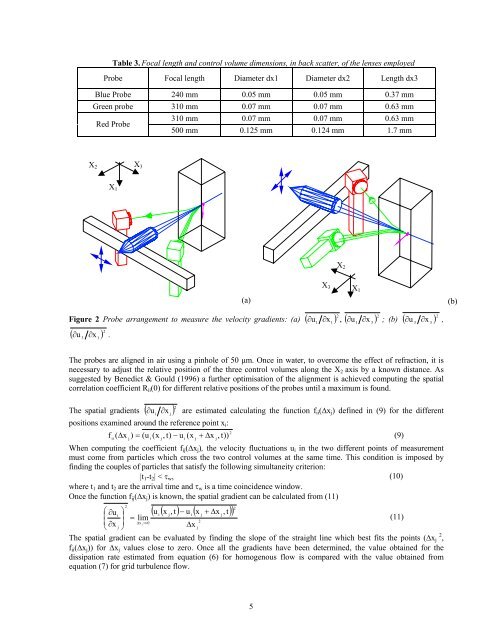
Table 3. Focal length and control volume dimensions, in back scatter, of the lenses employed Probe Focal length Diameter dx1 Diameter dx2 Length dx3 Blue Probe 240 mm 0.05 mm 0.05 mm 0.37 mm Green probe 310 mm 0.07 mm 0.07 mm 0.63 mm Red Probe 310 mm 0.07 mm 0.07 mm 0.63 mm 500 mm 0.125 mm 0.124 mm 1.7 mm X 3 X 2 X 1 X 2 X 3 X 1 (a) (b) 2 Figure 2 Probe arrangement to measure the velocity gradients: (a) ( ∂ u x ) , ( ∂ u ∂ ) 2 ; (b) ( u ∂ ) 2 ( u ∂ ) 2 ∂ . 3 x 1 1 ∂ 1 1 x 3 ∂ , 3 x 3 The probes are aligned in air using a pinhole of 50 µm. Once in water, to overcome the effect of refraction, it is necessary to adjust the relative position of the three control volumes along the X 2 axis by a known distance. As suggested by Benedict & Gould (1996) a further optimisation of the alignment is achieved computing the spatial correlation coefficient R ii (0) for different relative positions of the probes until a maximum is found. The spatial gradients ( u ∂ ) 2 ∂ are estimated calculating the function f ii (∆x j ) defined in (9) for the different i x j positions examined around the reference point x i : f 2 ( x ) = (u (x , t) − u (x + ∆x , t)) ii j i j i j j ∆ (9) When computing the coefficient f ij (∆x j ), the velocity fluctuations u i in the two different points of measurement must come from particles which cross the two control volumes at the same time. This condition is imposed by finding the couples of particles that satisfy the following simultaneity criterion: |t 1 -t 2 | < τ w , (10) where t 1 and t 2 are the arrival time and τ w is a time coincidence window. Once the function f ij (∆x j ) is known, the spatial gradient can be calculated from (11) 2 ( u ( x , t) − u ( x + ∆x , t ) 2 ⎛ u ⎞ i j i j j ⎜ ∂ i ⎟ = lim (11) x 0 2 j x ∆ ⇒ ⎝ ∂ j ⎠ ∆x j The spatial gradient can be evaluated by finding the slope of the straight line which best fits the points (∆x 2 j , f ii (∆x j )) for ∆x j values close to zero. Once all the gradients have been determined, the value obtained for the dissipation rate estimated from equation (6) for homogenous flow is compared with the value obtained from equation (7) for grid turbulence flow. 5
Page 1 and 2: Direct Measurement of the Turbulent
Page 3: Mohamed & LaRue (1990) performed an
Page 7 and 8: the two probes are aligned at the s
Page 9 and 10: ε M/ U 1 3 1E-4 Larue Re M = 6000
Page 11 and 12: 6. Conclusions A LDA method to meas

download

Create successful ePaper yourself

Delete template?

Save as template?