download

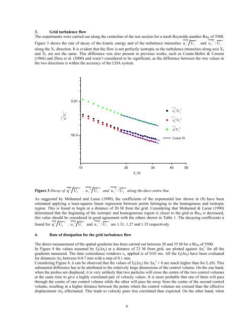
3. Grid turbulence flow
The experiments were carried out along the centreline of the test section for a mesh Reynolds number Re M of 5500.
2
2
Figure 3 shows the rate of decay of the kinetic energy and of the turbulence intensities u1 U1
and u
3
/ U
1
along the X 1 direction. It is evident that the flow is not perfectly isotropic as the turbulence intensities along axis X 1
and X 3 are not the same. This difference was also present in previous works, such as Comte-Bellot & Corssin
(1966) and Zhou et al. (2000) and wasn’t considered to be significant, as the difference between the rms values in
the two directions is within the accuracy of the LDA system.
2
2
0.01
u i
2
/U1
2
u 1 2 /U 1
2
u 3 2 /U 1
2
1E-3
q 2 /U 1
2
Linear fit
10 20 30 40 50
X 1
/M
Figure 3 Decay of q
2
U
1
2
2
, u
1
U1
and u
2
2 2
3
/ U1
along the duct centre line
As suggested by Mohamed and Larue (1990), the coefficients of the exponential law shown in (8) have been
estimated applying a least-squares linear regression between points belonging to the homogenous and isotropic
region. This is found to begin at a distance of 20 M from the grid. Considering that Mohamed & Larue (1990)
determined that the beginning of the isotropic and homogeneous region is closer to the grid as Re M is decreased,
this value should be considered in good agreement with the others shown in Table 1. The decaying coefficients n
2
found for q U 2 2
, u U 2
2
2
and u / are 1.31, 1.27 and 1.35 respectively.
1
1
1
3
U
1
4. Rate of dissipation for the grid turbulence flow
The direct measurement of the spatial gradients has been carried out between 20 and 35 M for a Re M of 5500.
In Figure 4 the values assumed by f ii (∆x j ) at a distance of 23 M from grid, are plotted against ∆x j 2 for all the
gradients measured. The time coincidence windows τ w applied is of 0.03 ms. All the f ii (∆x j ) have been evaluated
for distances ∆x j between 0-0.7 mm with a step of 0.1 mm.
Considering Figure 4, it can be observed that the values of f ii (∆x i ) for ∆x j 2 > 0 are much higher than for f 11 (0). This
substantial difference has to be attributed to the relatively large dimensions of the control volume. On the one hand,
when the probes are displaced, it is very unlikely that two particles will cross the centre of the two control volumes
at the same time to give a highly correlated pair of velocity values. It is more probable that one of them will pass
through the centre of one control volume while the other will pass far away from the centre of the second control
volume, resulting in a higher distance between the points where the control volumes are crossed than the effective
displacement ∆x j effectuated. This leads to velocity pairs less correlated than expected. On the other hand, when
6