A Variable Step-Size Selection Method for Implicit Integration ...

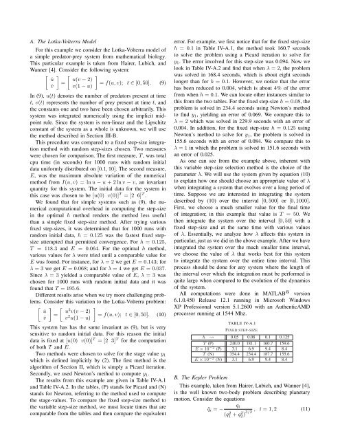
A. The Lotka-Volterra Model
For this example we consider the Lotka-Volterra model of
a simple predator-prey system from mathematical biology.
This particular example is taken from Hairer, Lubich, and
Wanner [4]. Consider the following system:
[ ] [ ]
u(v − 2)
=
= f(u, v); t ∈ [0, 50]. (9)
˙u˙v v(1 − u)
In (9), u(t) denotes the number of predators present at time
t, v(t) represents the number of prey present at time t, and
the constants one and two have been chosen arbitrarily. This
system was integrated numerically using the implicit midpoint
rule. Since the system is non-linear and the Lipschitz
constant of the system as a whole is unknown, we will use
the method described in Section III-B.
This procedure was compared to a fixed step-size integration
method with random step-sizes chosen. Two measures
were chosen for comparison. The first measure, T , was total
cpu time (in seconds) for 1000 runs with random initial
data uniformly distributed on [0.1, 10]. The second measure,
E, was the maximum absolute variation of the numerical
method from I(u, v) = ln u − u + 2 ln v − v, an invariant
quantity for this system. The initial data for the system in
this case was chosen to be [u(0) v(0)] T = [2 6] T .
We found that for simple systems such as (9), the numerical
computational overhead in computing the step-size
in the optimal h method renders the method less useful
than a simple fixed step-size method. After trying various
fixed step-sizes, it was determined that for 1000 runs with
random initial data, h = 0.125 was the fastest fixed stepsize
attempted that permitted convergence. For h = 0.125,
T = 118.3 and E = 0.064. For the optimal h method,
various values for λ were tried until a comparable value for
E was found. For instance, for λ = 2 we get E = 0.143; for
λ = 3 we get E = 0.068; and for λ = 4 we get E = 0.037.
Since λ = 3 yielded a comparable value of E, λ = 3 was
chosen for 1000 runs with random initial data and it was
found that T = 195.6.
Different results arise when we try more challenging problems.
Consider this variation to the Lotka-Volterra problem:
[ ] [ ]
u
= ˙u˙v
2 v(v − 2)
v 2 = f(u, v); t ∈ [0, 50]. (10)
u(1 − u)
This system has has the same invariant as (9), but is very
sensitive to random initial data. For this reason the initial
data is fixed at [u(0) v(0)] T = [2 3] T for the computation
of both T and E.
Two methods were chosen to solve for the stage value y 1
which is defined implicitly by (2). The first method is the
algorithm of Section II, which is simply a Picard iteration.
Secondly, we used Newton’s method to compute y 1 .
The results from this example are given in Table IV-A.1
and Table IV-A.2. In the tables, (P) stands for Picard and (N)
stands for Newton, referring to the method used to compute
the stage-values. To compare the fixed step-size method to
the variable step-size method, we must locate times that are
comparable from the tables and then compare the equivalent
error. For example, we first notice that for the fixed step-size
h = 0.1 in Table IV-A.1, the method took 160.7 seconds
to solve the problem using a Picard iteration to solve for
y 1 . The error involved for this step-size was 0.094. Now we
look in Table IV-A.2 and find that when λ = 2, the problem
was solved in 168.4 seconds, which is about eight seconds
longer than for h = 0.1. However, we notice that the error
has been reduced to 0.004, which is about 4% of the error
from when h = 0.1. We can locate other instances similar to
this from the two tables. For the fixed step-size h = 0.08, the
problem is solved in 234.4 seconds using Newton’s method
to find y 1 , yielding an error of 0.069. We compare this to
λ = 2 which was solved in 229.9 seconds with an error of
0.004. In addition, for the fixed step-size h = 0.125 using
Newton’s method to solve for y 1 , the problem is solved in
155.6 seconds with an error of 0.084. We compare this to
λ = 1 in which the problem is solved in 151.6 seconds with
an error of 0.025.
As one can see from the example above, inherent with
this variable step-size selection method is the choice of the
parameter λ. We will use the system given by equation (10)
to explain how one should choose an appropriate value of λ
when integrating a system that evolves over a long period of
time. Suppose we are interested in integrating the system
described by (10) over the interval [0, 500] or [0, 1000].
First, we choose a much smaller value for the final time
of integration; in this example that value is T = 50. We
then integrate the system over the interval [0, 50] with a
fixed step-size and at the same time with various values
of λ. Essentially, we analyze how λ affects this system in
particular, just as we did in the above example. After we have
integrated the system over the much smaller time interval,
we choose the value of λ that works best for this system
to integrate the system over the entire time interval. This
process should be done for any system where the length of
the interval over which the integration must be performed is
quite large when compared to the evolution of the dynamics
of the system.
All computations were done in MATLAB R version
6.1.0.450 Release 12.1 running in Microsoft Windows
XP Professional version 5.1.2600 with an AuthenticAMD
processor running at 1544 Mhz.
TABLE IV-A.1
FIXED STEP-SIZE
h → 0.05 0.08 0.1 0.125
T (P) 240.0 181.1 160.7 159.6
E × 10 −2 (P) 3.1 6.9 9.4 8.4
T (N) 354.4 234.4 187.7 155.6
E × 10 −2 (N) 3.1 6.9 9.4 8.4
B. The Kepler Problem
This example, taken from Hairer, Lubich, and Wanner [4],
is the well known two-body problem describing planetary
motion. Consider the equations
¨q i = −
q i
(q1 2 + , i = 1, 2 (11)
q2 2 )3/2