
You also want an ePaper? Increase the reach of your titles
YUMPU automatically turns print PDFs into web optimized ePapers that Google loves.
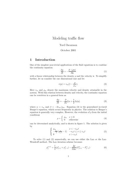
<strong>Modeling</strong> <strong>traffic</strong> <strong>flow</strong><br />
Tord Oscarsson<br />
October 2001<br />
1 Introduction<br />
One of the simplest non-trivial applications of the fluid equations is to combine<br />
the continuity equation<br />
∂ρ · (ρv)<br />
= −∂ (1)<br />
∂t ∂x<br />
with a linear relationship between the density ρ and the velocity v. To simplify<br />
further, let us consider the one dimensional case and let<br />
v(ρ) = v m (1 − ρ<br />
ρ m<br />
). (2)<br />
Here v m and ρ m denote the maximum velocity and density attainable in the<br />
system. With this relation between density and velocity, the continuity equation<br />
can be rewritten in a general form as<br />
∂ρ<br />
∂t = − ∂<br />
∂x [(α + 1 βρ)ρ], (3)<br />
2<br />
where α = v m and β = −2v m /ρ m . Equation (3) is the generalized in-viscid<br />
Burger’s equation, which occurs frequently in physics. The solution to Burger’s<br />
equation is generally very complex. However, the evolution of ρ from the initial<br />
conditions<br />
{<br />
ρm x ≤ 0<br />
ρ =<br />
(4)<br />
0 otherwise<br />
can be determined analytically, and is shown in figure 1. The solution is given<br />
by<br />
⎧<br />
⎨ ρ m<br />
x < −v m t<br />
− ρm 2<br />
⎩<br />
( x<br />
v − 1) −v mt mt ≤ x ≤ v m t<br />
(5)<br />
0 x > v m t<br />
To solve (1) and (2) numerically, we can use either the Lax or the Lax-<br />
Wendroff method. The Lax iteration scheme becomes<br />
ρ n+1<br />
j<br />
= 1 2 (ρn j+1 + ρn j−1 ) − ∆t<br />
2∆x (F n j+1 − F n j−1 ) (6)<br />
1
ρ(x,t)<br />
t > 0<br />
1<br />
t 2<br />
> t 1<br />
x<br />
.<br />
Figure 1: Solution to Burger’s equation for the initial conditionsin (4)<br />
where<br />
F (ρ) = ρv(ρ) (7)<br />
is the mass flux, and Fj<br />
n = F (ρ(x j , t n )). The Lax-Wendroff iteration scheme is<br />
given by<br />
ρ n+1<br />
j = ρ n j − ∆t<br />
+ 2<br />
( ∆t<br />
2∆x<br />
2∆x (F j+1 n − F j−1 n )<br />
) 2 [ ]<br />
qj+1/2 n (F j+1 n − F j n ) − qn j−1/2 (F j n − F j−1 n )<br />
(8)<br />
where<br />
Exercise 1<br />
q n j<br />
= ( dF<br />
dρ )n j . (9)<br />
Write a computer program for solving Burger’s equation along the lines described<br />
above. Implement both the Lax and the Lax-Wendroff scheme, and<br />
employ periodic boundary conditions.<br />
Test your program by solving for the initial conditions<br />
{<br />
ρm for L/4 ≤ x ≤ 3L/4<br />
ρ(x, t = 0) =<br />
0 otherwise<br />
(10)<br />
where L is the length of the system. The solution obtained for these initial<br />
conditions is similar to the solution in figure 1. The density will decrease linearly<br />
2
etween two points moving along the x-axis. This continues until the density<br />
at x = L/4 begins to change. After this, the solution is difficult to predict<br />
analytically. Use L = 400 m, v m = 25 m/s, ρ m = 1 arbitrary units, and the<br />
number of grid points NG = 40.<br />
Question 1:<br />
What time step should you use in this case?<br />
Question 2:<br />
The above initial condition has a peculiar effect in the Lax-Wendroff scheme.<br />
What happens and why? Suggest a way of altering the initial conditions slightly<br />
that will get rid of this effect.<br />
Run the program until the density at x = L/4 is beginning to change. Plot<br />
ρ, v, and F as functions of x for various times. Does the solution evolve as<br />
in figure 1 for a) the Lax scheme? b) the Lax-Wendroff scheme? Can you see<br />
any difference in the solutions obtained with the two methods? Try increasing<br />
the step length ∆t, keeping NG fixed. What happens? Also, try increasing NG<br />
while keeping ∆t fixed. What happens?<br />
Exercise 2<br />
Burger’s equation is often used as a first approximation of high-way <strong>traffic</strong> <strong>flow</strong><br />
(really the <strong>flow</strong> on a one-way road without car-passing capabilities). Which<br />
<strong>traffic</strong> situation can be modeled by the solution obtained in exercise 1?<br />
Run your program as in exercise 1. Use only the Lax-Wendroff method and<br />
use a Gaussian initial density<br />
ρ(x, t = 0) = ηρ m exp[−((x − L/4)/(L/8)) 2 ]. (11)<br />
where η is a constant 0 < η ≤ 1. In <strong>traffic</strong> this type of perturbation can occur<br />
where a slip road is feeding <strong>traffic</strong> onto the high-way. The cars already on the<br />
high-way break to allow cars to move onto the road, creating a concentration of<br />
cars close to the slip road. Use the same parameters as in exercise 1, and choose<br />
η = 0.1. Run the simulation with NT = 30 and the same ∆t as in the previous<br />
exercise. What is the duration in seconds of this simulation. What happens to<br />
the density perturbation in this time? Also, examine the velocity profile. Are<br />
these realistic, considering the <strong>traffic</strong> application?<br />
Run the program again, but with η = 0.9, corresponding to a car density<br />
close to maximum at x = L/4. How does the result differ from the η = 0.1 case.<br />
What <strong>traffic</strong> situation could this solution correspond to?<br />
3
2 Presentation of results<br />
Collect your results in a brief report where you present your figures, and comments<br />
to the figures, answers to questions in the instructions, and a listing of<br />
your computer program. Do not hand in more then about 10 figures, but try to<br />
chose figures that illustrate interesting features.<br />
4