Binomial Distributions
Binomial Distributions
Binomial Distributions

You also want an ePaper? Increase the reach of your titles
YUMPU automatically turns print PDFs into web optimized ePapers that Google loves.
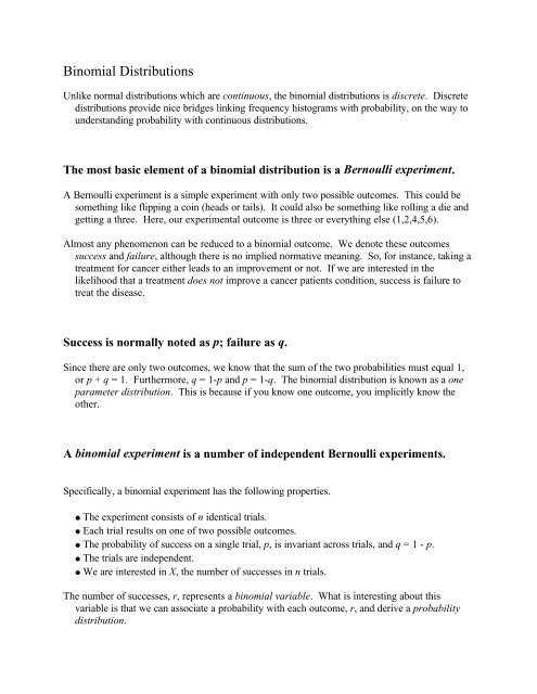
<strong>Binomial</strong> <strong>Distributions</strong><br />
Unlike normal distributions which are continuous, the binomial distributions is discrete. Discrete<br />
distributions provide nice bridges linking frequency histograms with probability, on the way to<br />
understanding probability with continuous distributions.<br />
The most basic element of a binomial distribution is a Bernoulli experiment.<br />
A Bernoulli experiment is a simple experiment with only two possible outcomes. This could be<br />
something like flipping a coin (heads or tails). It could also be something like rolling a die and<br />
getting a three. Here, our experimental outcome is three or everything else (1,2,4,5,6).<br />
Almost any phenomenon can be reduced to a binomial outcome. We denote these outcomes<br />
success and failure, although there is no implied normative meaning. So, for instance, taking a<br />
treatment for cancer either leads to an improvement or not. If we are interested in the<br />
likelihood that a treatment does not improve a cancer patients condition, success is failure to<br />
treat the disease.<br />
Success is normally noted as p; failure as q.<br />
Since there are only two outcomes, we know that the sum of the two probabilities must equal 1,<br />
or p + q = 1. Furthermore, q = 1-p and p = 1-q. The binomial distribution is known as a one<br />
parameter distribution. This is because if you know one outcome, you implicitly know the<br />
other.<br />
A binomial experiment is a number of independent Bernoulli experiments.<br />
Specifically, a binomial experiment has the following properties.<br />
• The experiment consists of n identical trials.<br />
• Each trial results on one of two possible outcomes.<br />
• The probability of success on a single trial, p, is invariant across trials, and q = 1 - p.<br />
• The trials are independent.<br />
• We are interested in X, the number of successes in n trials.<br />
The number of successes, r, represents a binomial variable. What is interesting about this<br />
variable is that we can associate a probability with each outcome, r, and derive a probability<br />
distribution.
Let's look at an easy example. If we toss a fair coin, defining getting a head on a toss as success,<br />
we know that p = 0.5 and q = 0.5. We propose to flip this coin four times; this is our binomial<br />
experiment. Each flip of the coin, or trial, constitutes a Bernoulli experiment.<br />
How do we enumerate success? We know that in four flips of the coin that there are five possible<br />
values of r; 0, 1, 2, 3, and 4. The binomial distribution associates a probability with each of<br />
these outcomes. So, for instance, what is the probability that r equals 4 [p(r=4)]? This is<br />
asking what is the probability of p(H and H and H and H). This is equal to (q)(q)(q)(q) = p 4 =<br />
0.5 4 = 0.0625. Thus, there is a 6.25% chance of tossing a coin four times and observing a head<br />
on each toss.<br />
What about getting one head and three tails [p(r=1)]? How many ways are there to get one head<br />
and three tails? We can list them as follows:
H T T T<br />
T H T T<br />
T T H T<br />
T T T H<br />
There are 4 ways to get 1 success<br />
and they have equal<br />
probability<br />
p(HTTT) = (p)(q)(q)(q) = pq 3 = (0.5)(0.5 3 ) = 0.0625<br />
p(THTT) = (q)(p)(q)(q) = pq 3 = (0.5)(0.5 3 ) = 0.0625<br />
p(TTHT) = (q)(q)(p)(q) = pq 3 = (0.5)(0.5 3 ) = 0.0625<br />
p(TTTH) = (q)(q)(q)(p) = pq 3 = (0.5)(0.5 3 ) = 0.0625<br />
Summing these independent probabilities we get 0.0625+0.0625+0.0625+0.0625 = 0.25. Thus,<br />
there is a 25% chance that in four flips, we observe a single head.
We can also use this method to calculate all the other probabilities for the values of r. But, there<br />
is a shortcut. What we are actually asking is, given 4 trials, how many ways can we distribute r<br />
successes across these trials. This then becomes a simple combination problem. The formula<br />
for combinations is:<br />
⎛n⎞<br />
⎜ ⎟ =<br />
⎝ r ⎠<br />
n!<br />
r!( n − r)!<br />
So, given all the possible values of r, we get:<br />
r<br />
0<br />
1<br />
2<br />
3<br />
4<br />
Combinations<br />
⎛4⎞<br />
⎜ ⎟ =<br />
⎝0<br />
⎠<br />
0!<br />
⎛4⎞<br />
⎜ ⎟ =<br />
⎝1⎠<br />
1!<br />
⎛4⎞<br />
⎜ ⎟ =<br />
⎝2<br />
⎠ 2!<br />
⎛4⎞<br />
⎜ ⎟ =<br />
⎝3⎠<br />
3!<br />
⎛4⎞<br />
⎜ ⎟ =<br />
⎝4<br />
⎠<br />
4!<br />
4!<br />
= 1<br />
0 !<br />
( 4 − )<br />
4!<br />
= 4<br />
1 !<br />
( 4 − )<br />
4!<br />
= 6<br />
2 !<br />
( 4 − )<br />
4!<br />
= 4<br />
3 !<br />
( 4 − )<br />
4!<br />
= 1<br />
4 !<br />
( 4 − )<br />
We can also use a general formula to calculate the individual probabilities associated with any one<br />
outcome of r. This formula is:<br />
p r q n-r<br />
Putting both this formula and that for combinations together, we get:<br />
⎛n⎞<br />
⎜ ⎟ p<br />
⎝ r ⎠<br />
r<br />
q<br />
n−r
⎛n⎞<br />
⎜ ⎟ p<br />
⎝ r ⎠<br />
r<br />
q<br />
n−r<br />
So, the full binomial probability distribution for this problem is given as:<br />
p(r) <strong>Binomial</strong> Probability<br />
⎛4⎞<br />
⎟⎠<br />
⎝0<br />
0<br />
4<br />
p(0) ⎜ ( 0.5 )( 0.5 )<br />
⎛4⎞<br />
⎟⎠<br />
⎝1<br />
1<br />
3<br />
p(1) ⎜ ( 0.5 )( 0.5 )<br />
⎛4⎞<br />
⎟⎠<br />
⎝2<br />
2<br />
2<br />
p(2) ⎜ ( 0.5 )( 0.5 )<br />
⎛4⎞<br />
⎟⎠<br />
⎝3<br />
p(3) ⎜ ( 0.5 )( )<br />
3 0. 5 1<br />
⎛4⎞<br />
⎟⎠<br />
⎝4<br />
4<br />
0<br />
p(4) ⎜ ( 0.5 )( 0.5 )<br />
0.0625<br />
0.2500<br />
0.3750<br />
0.2500<br />
0.0626<br />
0.50<br />
<strong>Binomial</strong> Distribution<br />
(n=3, p=0.33, q=0.67)<br />
Probability of Successe<br />
0.40<br />
0.30<br />
0.20<br />
0.10<br />
0.00<br />
0 1 2 3 4<br />
Number of Successes