Experiment 6: Constructing a Microscope

Experiment 6: Constructing a Microscope
Pre-lab Preparation:
• Review the following sections from the Young and Freedman textbook (page references
given for 12 th edition):
o Section 34.4: Thin Lenses, p. 1174 – 1182
o Section 34.7: The Magnifier, p. 1189 – 1190
o Section 34.8: Microscopes and Telescopes, p. 1191 – 1192
• Complete question 34.108 from the textbook
• Read the overview below, and roughly plan how to construct a microscope
Overview:
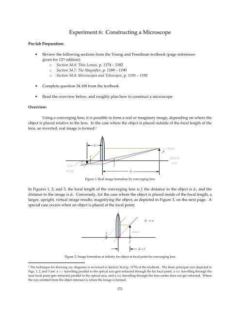
Using a converging lens, it is possible to form a real or imaginary image, depending on where the
object is placed relative to the lens. In the case where the object is placed outside of the focal length of the
lens, an inverted, real image is formed: 1
di
object
real
image
f
f
do
optical
axis
Figure 1: Real image formation by converging lens
In Figures 1, 2, and 3, the focal length of the converging lens is f, the distance to the object is do, and the
distance to the image is di. Conversely, for the case where the object is placed inside of the focal length, a
larger, upright, virtual image results, magnifying the object, as depicted in Figure 3, on the next page. A
special case occurs when an object is placed at the focal point:
di → ∞
f
object
f
do = f
Figure 2: Image formation at infinity for object at focal point for converging lens
1
The technique for drawing ray diagrams is reviewed in Section 34.4 (p. 1179) of the textbook. The three principal rays depicted in
Figs. 1, 2, and 3 are: a ray travelling parallel to the optical axis gets refracted through the far focal point, a ray travelling through the
near focal point gets refracted parallel to the optical axis, and a ray travelling through the lens centre does not get refracted. Where
the rays emitted from the object intersect is where the image is formed.
(1)

virtual
image
object
f
do
f
di
Figure 3: Virtual image formation by converging lens
When the object is located at the converging lens’ focal point, as in Figure 2, the rays forming the image
are parallel; thus, an image of infinite linear magnification is formed. This behaviour is quantified by the
thin lens equation, relating the object distance, do, the image distance, di, and the focal length of the lens:
1 1 1
= +
(1)
f d
0
d i
This equation is derived in Young and Freedman, 12 th Edition, p. 1174 – 1175 using a similar triangles argument.
The sign convention used by the textbook stipulates that f > 0 for a converging lens, and di > 0 if
the image is formed on the opposite side of the lens as the object (i.e. a real image). The behaviour in Figure
1 is observed if do > f, giving di > 0. Conversely, if do < f, then di < 0, giving the virtual image illustrated
in Figure 2. Finally, if do = f, then di → ∞ to give 1/di = 0.
Next, two types of magnification may be defined: the linear (or lateral) magnification, and the angular
magnification. The linear magnification, m, is the negative ratio of the object’s height to the image’s
height:
hi
m = −
h
o
Making use of similar triangles in the previous figures gives that the linear magnification is also the ratio
of the image distance to the object distance:
m
d
d
i
= −
(2)
o
If one solves for di in the thin lens equation, Eq. (1), and substitutes it into the expression for lateral magnification,
Eq. (2), then:
f
m = (3)
f −
d o
(2)

Hence, if an object is placed at the focal point, do = f, the lateral magnification approaches infinity, as noted
earlier. It’s clear, however, that placing an object at the focal point of a magnifying glass does not produce
an image of the object that’s infinitely large, so an alternate measure of magnification must be defined.
This is where the angular magnification is useful. The angular magnification, M, is defined as the
ratio of the angles subtended by the object and its magnified image:
θo
object
f
θi
d
(usually defined
as d = 25 cm)
parallel rays
focused by eye
f
object
Figure 4: Comparison of angle subtended by object and magnified object
θi
M =
θ
o
−1
tan ( ho
=
−1
tan ( h
o
/ f )
/ d)
For small angles θo and θi, tanθo ≈ θo and tanθi ≈ θi, leaving the following expression for the angular magnitude:
d
M = (4)
f
For convenience and consistency, most microscopes define angular magnification with d = 25 cm, the
minimum distance from the eye at which objects can be resolved for most people. It can be seen that, in
principle, as the focal length approaches zero, the angular magnification approaches infinity. The magnification
is actually limited by effects such as wavelength-dependent index of refraction and irregularities
in the shape of the lens that make the image irresolvable for M > 5 or so. To address this, a compound
microscope, making use of two converging lenses, is constructed:
eyepiece
Do
di
f
F
objective lens
f
do
Di
Figure 5: Sample microscope apparatus
(3)

Do
eyepiece
F
di
f
objective lens
f
do
Di → ∞
Figure 6: Alternate sample microscope
In both Figures 5 and 6, the objective lens, the converging lens with focal length f, is placed closest to the
object, and produces a real, inverted image of the object at distance di. This real image is then magnified,
either by putting it inside the focal length, F, of the eyepiece (as in Figure 5), or right inside the focal length
(as in Figure 6). One multiplies the linear magnification of each lens to find the total magnification of the
system in the case of Figure 5, but for Figure 6, the linear magnification of the eyepiece approaches infinity,
so the magnification is the product of the linear magnification of the objective lens, and the angular
magnification of the eyepiece. These expressions are given below:
F
F − D
µ = m m =
( Fig.
5)
o e
(5)
o
f
f − d
o
f d
= m M =
( Fig.
6 o e
(6)
f − d F
µ
)
o
Do is the distance between the eyepiece and the real image produced by the objective lens, which can be
found by considering the distance between the objective lens and the actual object, do, and applying the
thin lens equation, Eq. (1).
Procedure
The goal of this experiment is to construct a microscope and quantify its magnification factor.
The necessary ingredients, including three converging lenses, a light source, a screen, an optical bench,
and various holders, will be made available. The three lenses have unknown focal lengths that must be
found experimentally by any method one finds practical. For planning purposes, it may be assumed that
the lenses have focal lengths of approximately 5 cm, 10 cm, and 15 cm. Once the focal lengths are known,
the microscope may be created, using the arrangement in Figure 6 or 7 as a rough guide. The magnification
of the microscope must be measured, somehow, so some thought must go into this. Attempting
question 34.108 from the textbook will help in designing the microscope and defining the magnitude.
Since this lab doesn’t specify a particular procedure to follow, a full write-up is warranted. Arrange
the write-up with sections like the ones given below:
• Abstract: summarize the goal and results of the investigation in a few sentences.
• Introduction: let readers know what you set out to do, and briefly give some general background
on thin lenses. More than a few paragraphs for this section are not necessary.
(4)

• Method: this section is important – specifically explain, with numbers and diagrams, how you
measured the focal length of the lenses, how you assembled the microscope, and how you measured
the magnification of the microscope.
• Results: summarize the analysed and processed results of your investigation, including the focal
lengths of the lenses, the dimensions of the microscope, and the magnification. Make sure to include
uncertainties for each of the reported quantities, and compare observed values to theoretical
equivalents wherever possible. Show calculations in a separate section or appendix if you
want.
• Error Analysis: this section is also important – for this lab, a formal, quantitative treatment of error
is necessary. Propagate error from measurements to calculated values using the general formula,
for a sample quantity f = f(x,y):
2
2
⎛ ∂f
⎞ ⎛ ∂f
⎞
2
2
∆ f = ( ∆x)
+ ⎜ ⎟ ( ∆y)
(7)
⎜ ⎟
⎝ ∂x
⎠
⎜ y ⎟
⎝ ∂ ⎠
In Eq. (7), ∆f is the error in the calculated value f, which relies on two measured quantities, x, and
y, with related uncertainties ∆x and ∆y, respectively. For example, the error in the focal length is
related to the error in the object distance and the image distance by the following:
1 1 1
= + →
f d o
d i
f
d d
i o
= f ( d , d ) =
o i
d + d
i
o
Thus, the focal length is a two-variable equation, as in Eq. (7). The required partial derivatives
are:
∂f
∂d
o
d ( d + d ) − d d
i i o i
=
2
( d + d )
i
o
o
=
( d
i
2
di
+ d )
o
2
∂f
∂d
i
=
2
do
d + d )
(
i o
2
If these are substituted into the equation for the uncertainty, then:
∆f
=
=
=
( d
2
⎛ ∂f
⎞
2
⎜ ( ∆d
)
o
d
⎟
⎝ ∂
o ⎠
4
4
d
2 d
i
o
2
( ∆d
) + ( ∆d
)
4 o
4 i
( d + d ) ( d + d )
i
i
1
+ d )
o
o
2
2
d ( ∆d
)
4
i
⎛ ∂f
⎞
2
+
⎜ ( ∆d
)
i
d
⎟
⎝ ∂
i ⎠
o
i
2
+ d
4
o
o
( ∆d
)
i
2
(8)
Hence, by estimating the error in the position of the object, ∆do, and the position of the image, ∆di,
the corresponding error in the focal length, ∆f, is found for that measurement. Note that, for the
focal length measurement for the lenses, you will want to average several values for f. Calculating
the uncertainty associated with each measurement, ∆f, allows values with large uncertainties
(5)

to be discarded. 2 The uncertainty in the averaged focal length value may then be roughly estimated
by the following ad-hoc formula:
f
avg
=
f1
+ f2
+ ... + fN
N
→
( ∆f
)
average
∆ ( favg)
=
(9)
N
Thus, the error in the averaged focal length value is given by the average of the error in the individual
values, divided by the root of the number of values examined, N.
Estimating the error in the magnification for the microscope, given by an equation like
Eq. (5) or (6) may be done in the same way as was demonstrated for the focal length, Eq. (8).
Make sure to comment on sources of error and justify the measurement uncertainties in each
case. For some measurements, the uncertainty may be larger than half of the smallest division on
the measuring device – explain why in each case.
• Conclusion/Discussion: briefly summarize what was found and restate the numbers and their
associated uncertainties. Mention particularly problematic parts of the investigation, and suggest
ways that the procedure may be improved, if someone were to try and repeat your experiment
for better results.
Conclusion:
Good luck! The tricky part of this investigation will likely be interpreting the data that is collected.
Performing the actual experiment should not be too difficult, but a bit of careful thought must go
into planning what to do to get useful data, and what to do with the data once it’s been collected to get
useful conclusions. This approximates research, where much effort goes into planning and justifying experiments,
and trying to learn things from them, as opposed to actually performing the experiments. Accordingly,
the mark for this investigation will be based more on one’s ability to create and justify an experimental
procedure, and quantify the results and uncertainties, as opposed to getting the correct results
– keep that in mind!
2
Strictly, one should find the weighted mean of the f-values, with the weightings being inversely proportional to the uncertainty for
each value; that is, wi = 1/∆fi. To save time, if the errors are about the same for each value, one can take the standard mean and estimate
the uncertainty in the average value using Eq. (9).
(6)