7. quantitative calcareous nannofossil biostratigraphy of ... - Ispra

Robertson, A.H.F., Emeis, K.-C., Richter, C., and Camerlenghi, A. (Eds.), 1998
Proceedings of the Ocean Drilling Program, Scientific Results, Vol. 160
7. QUANTITATIVE CALCAREOUS NANNOFOSSIL BIOSTRATIGRAPHY OF PLIOCENE
AND PLEISTOCENE SEDIMENTS FROM THE ERATOSTHENES SEAMOUNT REGION
IN THE EASTERN MEDITERRANEAN 1
T. Scott Staerker 2,3
ABSTRACT
Quantitative methods were used to document the abundance patterns of selected Pleistocene and Pliocene calcareous nannofossil
species from four Ocean Drilling Program sites in the Eratosthenes Seamount region of the Eastern Mediterranean.
Results show that many similarities exist between the species abundance patterns reported in this study and the abundance patterns
from other geologic sequences in the Western and Central Mediterranean. Unconformities, likely associated with Pleistocene
tectonic movement of the subducting Eratosthenes Seamount, limit the correlation of some biostratigraphic events.
Despite the limitations caused by local tectonic erosion at Sites 965, 966, and 968, the geologic section recovered from Site 967
appears minimally affected and presents a high-resolution reference section for the Eastern Mediterranean. Three biostratigraphic
events are proposed to refine correlation of the Pliocene geologic sections in the Eastern Mediterranean.
INTRODUCTION
Ocean Drilling Program (ODP) Leg 160 drilled holes at 11 sites
in the Central and Eastern Mediterranean Sea. This study details the
quantitatively derived abundance patterns of selected Pleistocene and
Pliocene calcareous nannofossil species observed in samples collected
from four of the Leg 160 sites.
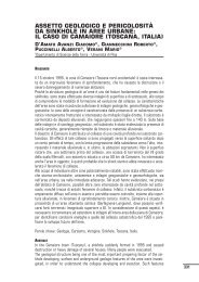
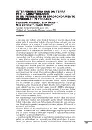
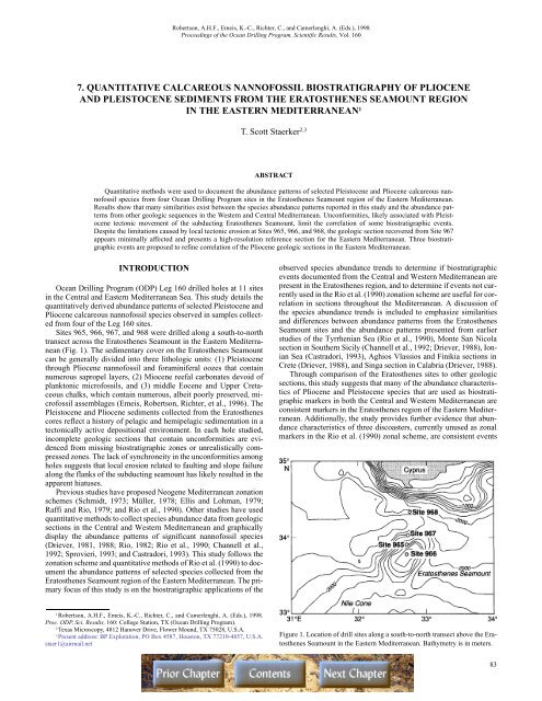
Sites 965, 966, 967, and 968 were drilled along a south-to-north
transect across the Eratosthenes Seamount in the Eastern Mediterranean
(Fig. 1). The sedimentary cover on the Eratosthenes Seamount
can be generally divided into three lithologic units: (1) Pleistocene
through Pliocene nannofossil and foraminiferal oozes that contain
numerous sapropel layers, (2) Miocene reefal carbonates devoid of
planktonic microfossils, and (3) middle Eocene and Upper Cretaceous
chalks, which contain numerous, albeit poorly preserved, microfossil
assemblages (Emeis, Robertson, Richter, et al., 1996). The
Pleistocene and Pliocene sediments collected from the Eratosthenes
cores reflect a history of pelagic and hemipelagic sedimentation in a
tectonically active depositional environment. In each hole studied,
incomplete geologic sections that contain unconformities are evidenced
from missing biostratigraphic zones or unrealistically compressed
zones. The lack of synchroneity in the unconformities among
holes suggests that local erosion related to faulting and slope failure
along the flanks of the subducting seamount has likely resulted in the
apparent hiatuses.
Previous studies have proposed Neogene Mediterranean zonation
schemes (Schmidt, 1973; Müller, 1978; Ellis and Lohman, 1979;
Raffi and Rio, 1979; and Rio et al., 1990). Other studies have used
quantitative methods to collect species abundance data from geologic
sections in the Central and Western Mediterranean and graphically
display the abundance patterns of significant nannofossil species
(Driever, 1981, 1988; Rio, 1982; Rio et al., 1990; Channell et al.,
1992; Sprovieri, 1993; and Castradori, 1993). This study follows the
zonation scheme and quantitative methods of Rio et al. (1990) to document
the abundance patterns of selected species collected from the
Eratosthenes Seamount region of the Eastern Mediterranean. The primary
focus of this study is on the biostratigraphic applications of the
observed species abundance trends to determine if biostratigraphic
events documented from the Central and Western Mediterranean are
present in the Eratosthenes region, and to determine if events not currently
used in the Rio et al. (1990) zonation scheme are useful for correlation
in sections throughout the Mediterranean. A discussion of
the species abundance trends is included to emphasize similarities
and differences between abundance patterns from the Eratosthenes
Seamount sites and the abundance patterns presented from earlier
studies of the Tyrrhenian Sea (Rio et al., 1990), Monte San Nicola
section in Southern Sicily (Channell et al., 1992; Driever, 1988), Ionian
Sea (Castradori, 1993), Aghios Vlassios and Finikia sections in
Crete (Driever, 1988), and Singa section in Calabria (Driever, 1988).
Through comparison of the Eratosthenes sites to other geologic
sections, this study suggests that many of the abundance characteristics
of Pliocene and Pleistocene species that are used as biostratigraphic
markers in both the Central and Western Mediterranean are
consistent markers in the Eratosthenes region of the Eastern Mediterranean.
Additionally, the study provides further evidence that abundance
characteristics of three discoasters, currently unused as zonal
markers in the Rio et al. (1990) zonal scheme, are consistent events
1
Robertson, A.H.F., Emeis, K.-C., Richter, C., and Camerlenghi, A. (Eds.), 1998.
Proc. ODP, Sci. Results, 160: College Station, TX (Ocean Drilling Program).
2
Texas Microscopy, 4812 Hanover Drive, Flower Mound, TX 75028, U.S.A.
3
Present address: BP Exploration, PO Box 4587, Houston, TX 77210-4857, U.S.A.
staer1@airmail.net
Figure 1. Location of drill sites along a south-to-north transect above the Eratosthenes
Seamount in the Eastern Mediterranean. Bathymetry is in meters.
83

T.S. STAERKER
that can used to further subdivide Pliocene biostratigraphy throughout
the Mediterranean.
SCIENTIFIC OBJECTIVES, METHODS,
AND BIOSTRATIGRAPHIC ZONATIONS
With the exception of the shallow-water carbonates at Site 965, all
of the cores recovered from Leg 160 sites were conducive to nannofossil
analysis. A total of 1275 samples from the Eratosthenes
Transect (Sites 965−968) were analyzed during this postcruise nannofossil
project. Samples were collected aboard ship by members of
the Shipboard Scientific Party. Sample spacing varied, but generally
included two samples per section of core, spaced ~75 cm apart. Because
the sample spacing was not adjusted to account for variations
in sedimentation rates, biostratigraphic resolution is reduced in intervals
with low-sedimentation rates relative to those intervals with
high-sedimentation rates.
Standard smear slides were prepared from the interior portions of
2-cm 3 sample tubes. Optical adhesive (Norland #61) was used as a
mounting medium for all of the smear slides. Taxon identifications
were performed using a Zeiss Universal microscope under magnifications
of approximately 1250× and 500×. The greater resolution
provided by a JEOL JSM3000 scanning electron microscope (SEM)
was used to verify the Emiliania huxleyi and large Gephyrocapsa
(>5.5 µm) datums from selected holes. A discussion of some species
and biostratigraphic definitions used in this study is found in the Appendix
in this chapter.
The nannofossil abundance data were compiled using a quantitative
method that involved point counts of selected species. Unlike the
Rio et al. (1990) study, which quantitatively documented a given species’
abundance using several methods over the same interval (such
as counting the number of specimens per fixed area of slide), this
study only used a single method for each taxon studied. Although the
total number of specimens counted differed between species, the
method used throughout this study involved counting an index species
vs. a fixed number of related forms. A discussion of the individual
criteria used for each species can be found in the Appendix. The
zonation scheme and datums identified in this study are shown in Figure
2.
Once determined through light microscopy, nannofossil abundance
data from all samples were entered into a Microsoft Excel
spreadsheet and eventually displayed as graphs using DeltaGraph
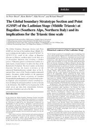
software. The abundance patterns of the Leg 160 material are shown
in Figures 3−6. The length and total values shown on the axes of all
graphs of a given species were kept constant so that abundance patterns
could be easily compared among holes. This graphical presentation
style limits the reader’s ability to accurately determine the precise
abundance values where abundance fluctuates significantly (i.e.,
G. oceanica), but enhances the ability to recognize fluctuation trends
for correlation among holes.
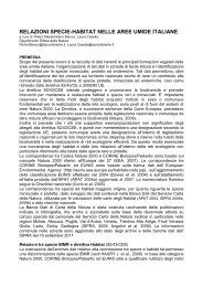
Many of the datums used in this study have been correlated with
global magnetostratigraphy and oxygen isotope stages (Backman and
Shackleton, 1983; Berggren et al., 1995; Cande and Kent, 1992,
1995; Shackleton et al., 1990; Sprovieri, 1993; Wei, 1993; Vergnaud-
Grazzini et al., 1994; Zijderveld et al., 1991). The age assignments
for all datums used in this study, including both zonal markers and
additional datums, are found in Table 1.
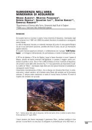
Figure 2. Pliocene and Pleistocene calcareous nannofossil zonation scheme
that shows zonal boundary datums and additional datums correlated to the
time scale of Berggren et al. (1995). FAD = first appearance datum, LAD =
last appearance datum, FCO = first common occurrence, and LCO = last
common occurrence.
A
0
10
20
30
40
50
60
70
80
90
100
0
30
25
20
15
10
5
35
40
0
5
0
20
40
G. oceanica
60
80
100
120
140
160
180
200
Gephyrocapsa sp. 3
large Gephyrocapsa (>5.5 µm)
C. macintyrei P. lacunosa
30
25
20
15
10
80
60
40
20
0
100
120
140
Depth (mbsf)
20 10 0
FAD
B
0
20
40
60
G. oceanica Gephyrocapsa sp. 3
large Gephyrocapsa (>5.5 µm)
C. macintyrei P. lacunosa
80
100
120
140
160
180
200
0
10
20
30
40
50
60
70
80
90
100
5
0
30
25
20
15
10
80
60
40
20
0
100
120
140
0
0
10
FAD
0
10
unconformity
LAD 92%
0
10
unconformity
0
10
LAD
20
20
20
20
40
35
30
25
20
15
10
5
0
0
Depth (mbsf)
30 20 10
0
0
0
FAD
10
20
30
FAD
10
20
30
FAD
LAD
10
20
30
LAD
10
20
30
LAD
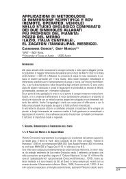
Figure 3. Graphs showing abundance patterns of biostratigraphically significant Pleistocene nannofossil species in samples collected from (A) Hole 965A and
(B) Hole 966D relative to depth (mbsf). Abundance is shown as total specimens counted vs. a fixed number of related forms as described in the Appendix.
84

CALCAREOUS NANNOFOSSIL BIOSTRATIGRAPHY
BIOSTRATIGRAPHIC INTERPRETATIONS
Hole 965A
Only one hole was drilled at Site 965. The hole consisted of 27
cores that reached a total depth of 240.40 mbsf. Lithologies ranged
from nannofossil ooze to clay in the upper four cores to packstones,
grainstones, and wackestones containing only benthic foraminifers,
mollusks, and algal laminations in Cores 160-965A-4H through 27X
(Emeis, Robertson, Richter, et al., 1996). During postcruise nannofossil
studies, 41 samples were analyzed from Core 160-965A-1H
through 4H. Graphs showing species abundance patterns are shown
in Figures 3 and 4.
Emiliania huxleyi is present from Sample 160-965A-1H-1, 15−16
cm (0.15−0.16 mbsf) through 2H-1, 20−22 cm (1.00−1.02 mbsf),
which indicates that these samples are in Zone MNN 21. The E. huxleyi
acme (Zone MNN 21b) was not identified in Hole 965A. The
scanning electron microscope (SEM) was used to verify the placement
of the first appearance datum (FAD) E. huxleyi.
In Sample 160-965A-2H-1, 109−110 cm (1.89−1.90 mbsf)
through 2H-2, 105−106 cm (3.35−3.36 mbsf) Zone MNN 20 is recognized
by the absence of both E. huxleyi and Pseudoemiliania lacunosa.
The accompanying assemblage includes Rhadosphaera claviger,
Gephyrocapsa oceanica, small gephyrocapsids, Calcidiscus
leptoporus, Syracosphaera pulchra, and Scapholithus fossilis. Although
it was not studied quantitatively, Helicosphaera kamptneri
was observed to fluctuate significantly throughout these samples. Reworked
Cretaceous, Eocene, and Pliocene species, in addition to
clay-sized and silt-sized calcite particles, also fluctuated throughout
these samples.
Pseudoemiliania lacunosa becomes a consistent part of the assemblage
beginning in Sample 160-965A-2H-3, 4−5 cm (3.84−3.85
mbsf). The presence of P. lacunosa means that this sample and those
immediately below are within Zone MNN 19f. Although rare specimens
of P. lacunosa were observed uphole, they were considered reworked.
With the exception of an abundance peak in Sample 160-
965A-2H-3, 90−91 cm (4.70 mbsf), the uppermost 2.5 m of this zone
is typified by low numbers of P. lacunosa (less than 2% P. lacunosa
per 500 total coccolith count). Below 4.70 mbsf, P. lacunosa is a
common part of the assemblage.
The last appearance datum (LAD) of Gephyrocapsa sp. 3, which
is reported by Rio et al., 1990 as an alternate marker within Zone
MNN 19f, was observed in Sample 160-965A-2H-3, 90−91 cm
(4.70−4.71 mbsf). The quantitative method for determining the presence
(or absence) of Gephyrocapsa sp. 3 follows the criteria of Rio et
al. (1990) and is described in the Appendix. The base of Zone MNN
19f, as indicated by the FAD of Gephyrocapsa sp. 3, is recognized in
Sample 160-965A-2H-4, 116−117 cm (6.46−6.47 mbsf). An increase
in abundance in P. lacunosa was also noticed at 6.46 mbsf. The recognition
of the FAD and LAD of Gephyrocapsa sp. 3 in successive
samples (1.08 m apart) suggests that either an unconformity exists
between these samples or the samples are within an interval characterized
by very low sedimentation rates (approximately 4.3 m/m.y.).
The next significant change in the nannofossil assemblage occurs
where large Gephyrocapsa (>5.5 µm) is recognized in Sample 160-
965A-2H-7, 28−29 cm (10.08−10.09 mbsf). Large Gephyrocapsa is
observed in only two samples. The FAD was identified in Sample
160-965A-2H-CC (10.28−10.30 mbsf), whereas the LAD was identified
in Sample 160-965A-2H-7, 28−29 cm (10.08−10.09 mbsf). Together,
these two samples comprise Zone MNN 19d.
In Sample 160-965A-3H-1, 21−22 cm (10.51−10.52 mbsf), Calcidiscus
macintyrei becomes a common part of the nannofossil assemblage.
Typically, the LAD of C. macintyrei signifies the top of
Zone 19b; however, the absence of G. oceanica in this sample indicates
that the sample is actually within Zone 19a. Collectively, the
FADs of large Gephyrocapsa and G. oceanica (Sample 160-965A-
2H-CC) juxtaposed to the LAD of C. macintyrei (160-965A-3H-1,
21−22 cm) in successive samples indicates that an unconformity exists
between 10.30 mbsf and 10.52 mbsf. Within the interval represented
by the unconformity, sediments comprising Zones MNN 19c
and MNN 19b are entirely missing, and portions of Zone MNN 19a
and MNN 19d may also be missing. The missing sediments represent
a length of time that ranges from a maximum of 1.10 Ma to 2.02 Ma,
to a minimum span from 1.47 Ma to 1.72 Ma (Fig. 2 and Table 1).
According to this interpretation, sediments spanning the Pleistocene/
Pliocene boundary are not present in Hole 965A.
In Sample 160-965A-3H-1, 135−136 cm (11.65−11.66), a nannofossil
assemblage typified by the presence of Discoaster brouweri
and Discoaster triradiatus is observed. Owing to the absence of other
discoasters, this sample is assigned to Pliocene Zone MNN 18. The
accompanying assemblage includes C. leptoporus, C. macintyrei,
small reticulofenestrids, and H. kamptneri.
Discoaster pentaradiatus is observed in Sample 160-965A-3H-3,
99−100 cm (14.29−14.30 mbsf), which marks the uppermost limit of
Zone 17−16b. At 15.72 mbsf, below the LAD of D. pentaradiatus,
the LAD of Discoaster surculus is observed. Discoaster surculus is
used in extra-mediterranean zonation schemes (Okada and Bukry,
1980; Martini,1971) as a zonal marker; however, in the Mediterranean,
the LADs of D. pentaradiatus and D. surculus are virtually indistinguishable
(Rio et al, 1990; Müller, 1978; Driever, 1981; and Ellis
and Lohman, 1979). Following the zonation scheme of Rio et al.
(1990), the two species are placed at the top of Zone MNN 17−16b.
In Sample 160-965A-3H-5, 96−97 cm (17.26−17.27), Discoaster
tamalis is observed in abundances greater than 2% of the total discoaster
population. Following the criteria of Rio et al. (1990), the
downhole increase in D. tamalis greater than 2% of the discoaster
population indicates that this sample is within Zone MNN 16a. All
occurrences of D. tamalis identified uphole were less than 2% and
thus, are considered above the datum. Because D. tamalis fluctuates
to rare or absent near its LAD, Rio et al. (1990) and Sprovieri (1993)
cite the importance of using a close sample spacing to accurately
identify the zonal boundary. The average sample spacing used in this
study was 74 cm, which is considerably greater than the average
spacings used by Rio et al. (1990) (40 cm to 10 cm) and Sprovieri
(1993) (25 cm) in their respective studies. For this reason, the LAD
of D. tamalis datum in this study may have been placed lower in the
geologic record compared to the Rio et al. (1990) and Sprovieri
(1993) studies. Discoaster tamalis remains a continual part of the
nannofossil assemblage downhole and increases in abundance near
30% of the total discoaster assemblage in Sample 160-965A-4H-1,
42−43 cm (20.22−20.23 mbsf). The increase in abundance of D. tamalis
is coincident with increases in the abundance of Discoaster
asymmetricus and a single spike in the abundance pattern of D. pentaradiatus.
In Sample 160-965A-4H-2, 29−30 cm (21.59−21.60
mbsf), immediately below the increases in D. tamalis and D. asymmetricus,
Sphenolithus abies/neoabies becomes a consistent part of
the assemblage. In addition to the LAD of Sphenolithus abies/neoabies,
assemblage changes that include the absence of both D. pentaradiatus
and D. tamalis, the dramatic decrease of D. asymmetricus,
and a marked increase in the abundance of D. surculus are observed
in Sample 160-965A-4H-2, 29−30 cm (21.59−21.60 mbsf). The absence
of D. pentaradiatus in the lowermost portion of Zone MNN
16a is a consistent event observed in the Central Mediterranean and
first described as a paracme event by Driever (1988). The assemblage
that includes D. tamalis in the absence of R. pseudoumbilicus and D.
pentaradiatus (paracme) is observed in only one sample in Hole
965A, which suggests that either the sedimentation rates are low or
erosion has removed most of the D. pentaradiatus paracme interval
in Hole 965A.
Reticulofenestra pseudoumbilicus (Zone MNN 14−15) is present
beginning in Sample 160-965A-4H-2, 97−98 cm (22.27−22.28
mbsf). In the following sample (23.15−23.16 mbsf), which is the
deepest sample studied in Hole 965A, another significant change in
85

T.S. STAERKER
A
D. brouweri
D. triradiatus
D. pentaradiatus
D. surculus
80
70
60
50
40
30
20
10
0
100
90
80
70
60
50
40
30
20
10
0
40
35
30
25
20
15
10
5
0
100
90
80
70
60
50
40
30
20
10
0
10
Depth (mbsf)
20
LAD
10
20
LAD
10
20
LAD
10
20
LAD
30
30
30
B
0
10
20
30
D. brouweri
40
50
60
70
80
90
100
0
5
D. triradiatus
25
20
15
10
30
35
40
0
10
D. pentaradiatus
40
30
20
70
60
50
80
90
100
0
10
20
D. surculus
50
40
30
60
70
80
70
70
70
40
70
60
50
60
60
40
60
30
30
30
30
20
20
20
20
LAD
LAD
LAD
LAD
50
40
50
40
50
C
D. brouweri
D. triradiatus
D. pentaradiatus
D. surculus
80
70
60
50
40
30
20
10
0
40
35
30
25
20
15
10
5
0
100
90
80
70
60
50
40
30
20
10
0
60
LAD
120
70
120
120
120
110
110
70
110
100
110
70
Depth (mbsf)
90
90
80
90
100
90
80
80
80
60
60
100
60
30
Depth (mbsf)
paracme
70
100
90
100
80
70
60
50
40
30
20
10
0
LAD
LAD
LAD
paracme
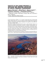
Figure 4. Graphs showing abundance patterns of selected Discoaster species in samples collected from (A) Hole 965A, (B) Hole 966D, and (C) Hole 967A relative
to depth (mbsf). Abundance for each species is shown as the percent of the total discoaster assemblage counted.
nannofossil assemblage is observed: P. lacunosa and D. asymmetricus
are absent, Discoaster variabilis becomes a significant part of the
discoaster assemblage (Fig. 4A), and Ceratolithus delicatus is observed
for the first time downhole. Collectively, the floral changes
suggest the presence of an unconformity in which some of Zones
MNN 15/14 and MNN 13 may be missing. A coincident minor lithologic
change typified by an abundance of calcite fragments is also observed
between 22.23 and 23−15 mbsf. Further discussion of all suspected
unconformities and comparisons with other Leg 160 holes are
located in the “Stratigraphic Discussion” section, which follows.
Hole 966D
Because Site 966 is at the crest of the seamount, it would be expected
to be least altered by slumping and faulting associated with
collapse of the seamount during subduction. Site 966 potentially offered
the most complete geologic section of Pleistocene and Pliocene
deposits of any of the sites along the Eratosthenes Seamount transect.
However, some missing intervals attributed to unconformities were
identified in Hole 966D during postcruise studies. The other holes at
Site 966D were not studied during postcruise research. Calcareous
86

CALCAREOUS NANNOFOSSIL BIOSTRATIGRAPHY
D. intercalaris
D. tamalis
D. asymmetricus
D. variablilis
60
55
50
45
40
35
30
25
20
15
10
5
0
50
45
40
35
30
25
20
15
10
5
0
50
45
40
35
30
25
20
15
10
5
0
40
35
30
25
20
15
10
5
0
Depth (mbsf)
20
30
30
10
10
20
20
0
5
10
15
D. tamalis
20
25
30
35
40
45
50
0
5
10
D. asymmetricus
15
20
25
30
35
40
45
50
D. variabilis
30
30
70 60 50 40
20
90 80 70 60
20
0
5
10
15
20
25
30
35
40
45
50
70 60 50 40
D. tamalis D. asymmetricus D. variabilis
0
5
10
15
20
25
35
30
40
45
50
120
120
110
110
100
100
30
10
0
5
D. intercalaris
25
20
15
10
30
35
40
120
110
100
30
30
20
20
30
10
LCO
20
LCO
0
5
10
15
20
25
30
35
40
45
50
55
60
Depth (mbsf) Depth (mbsf)
70 60 50 40
90 80 70 60
90 80 70 60
0
5
D. intercalaris
25
20
15
10
30
35
40
LCO
LCO
70 60 50 40
90 80 70 60
0
5
10
LCO
15
20
25
30
35
40
120
110
100
45
50
55
60
LCO
Figure 4 (continued).
nannofossil abundance patterns for Hole 966D are shown in Figures
3B and 4B.
Pleistocene hemipelagic oozes comprise the uppermost cores
from Hole 966D. The interval from Sample 160-966D-1H-1, 60−61
(0.60−0.61 mbsf) to Sample 160-966D-2H-1, 125−126 cm (4.75−
4.76 mbsf) contains a rare to common, well-preserved nannofossil assemblage
typical of the uppermost Pleistocene Zone MNN 21, as indicated
by the presence of E. huxleyi. Core 160-966D-1H contains
some reworked Pliocene, Eocene, and Cretaceous taxa, in addition to
abundant silt- and clay-sized calcite fragments of unknown origin.
Gephyrocapsa oceanica, small and medium gephyrocapsids (

T.S. STAERKER
A
0
20
40
60
G. oceanica Gephyrocapsa sp. 3
large Gephyrocapsa (>5.5 µm)
C. macintyrei
P. lacunosa
80
100
120
140
160
180
200
0
10
20
30
40
50
60
70
80
90
100
30
25
20
15
10
5
0
40
35
30
25
20
15
10
5
0
100
80
60
40
20
0
120
140
60
40
20
Depth (mbsf)
30
30
30
30
30
50
50
10
50
0
0
20
40
60
80
100
120
140
160
180
200
60
40
10
0
60
40
50
20
10
0
120
100
80
60
40
20
0
140
60
40
10
0
60
40
20
10
0
25
20
15
10
5
0
40
35
30
25
20
15
10
5
0
30
60
40
10
0
60
40
20
10
0
0
10
20
30
40
50
60
70
80
90
100
Depth (mbsf)
30 20
60
50
60
40
20
20
30
40
10
10
30
0
0
50
60
50
40
20
10
0
LAD
FAD
LAD
FAD
20
30
50
FAD
50
LAD
B
20
G. oceanica Gephyrocapsa sp. 3
large Gephyrocapsa (>5.5 µm)
C. macintyrei
P. lacunosa
30
50
FAD
LAD
LAD
FAD
FAD
reworking
Figure 5. Graphs showing abundance patterns of biostratigraphically significant Pleistocene nannofossil species in samples collected from (A) Hole 967C and
(B) Hole 968A relative to depth (mbsf). Abundance is shown as total specimens counted vs. a fixed number of related forms as described in the Appendix.
from 160-966D-2H-2, 51−52 cm (5.51−5.52 mbsf) through 2H-5,
125−126 cm (10.75−10.76 mbsf) lack both E. huxleyi and P. lacunosa;
therefore, these samples are assigned to the upper Pleistocene
Zone MNN 20. A typical assemblage within this zone consists of G.
oceanica, small and medium gephyrocapsids (5.5 µm). This interval also lacks G. oceanica. The
remaining assemblage is similar to that found in the preceding zone.
The LAD of large Gephyrocapsa (>5.5 µm) occurs in Sample
160-966D-3H-7, 60−61 (22.60-22.61 mbsf). Large Gephyrocapsa
remains a part of the assemblage through Sample 160-966D-4H-1,
60−61 cm (24.60−24.61 mbsf). Because only a minor size variation
was detected in the light microscope below the FAD of large Gephyrocapsa,
(>5.5 µm), five samples spanning the FAD were studied under
the SEM for confirmation. In the SEM study, 100 gephyrocapsid
specimens larger than 4.0 µm were counted to document the presence
of gephyrocapsid forms larger than 5.5 µm. Because no specimens
larger than 5.5 µm were observed below the boundary, the SEM study
confirmed the placement of the boundary as previously defined by
use of the light microscope. All samples that included large Gephyrocapsa
(>5.5 µm) were assigned to Zone MNN 19d.
In Sample 160-966D-4H-2, 129−130 cm (25.29−25.30 mbsf), the
absence of large Gephyrocapsa (>5.5 µm) and the next downhole
marker, C. macintyrei indicates Zone MNN 19c. The next significant
change in the microfloral assemblage occurs in Sample 160-966D-
4H-3, 47−48 cm, (25.97−25.98 mbsf) where the LAD of C. macintyrei
and the FAD of G. oceanica are observed. This sample is assigned
to Zone MNN 19b. The co-occurrence of C. macintyrei and G. oceanica
in the same sample combined with Zone MNN 19c being represented
by only one sample indicates that most of Zone 19b is missing
(0.16 to 0.60 Ma). It is likely that some of the overlying or underlying
zones are also missing. Because the single sample represents
the lowermost Pleistocene Zone 19b, it is uncertain whether the
Pleistocene/Pliocene boundary is present in Hole 966D or if the
boundary is represented by an unconformity.
Uppermost Pliocene Zone MNN 19a, defined by the absence of
both G. oceanica and D. brouweri, is recorded from Samples 160-
966D-4H-3, 125−126 cm (26.75 mbsf) through 4H-4, 62−63 cm
(27.62 mbsf).
In Sample 160-966D-4H-4, 122−123 cm (28.22 mbsf) the LADs
of D. brouweri and D. triradiatus were identified. Although very rare
occurrences of other discoasters were observed in some samples, D.
brouweri and D. triradiatus were interpreted to be the only in situ discoasters
in the interval from 160-966D-4H-4, 122−123 (28.22−28.23
mbsf) through 160-966D-5H-1, 125−126 cm (33.25−33.26 mbsf),
thus indicating that these samples are within Zone MNN 18.
Discoaster pentaradiatus becomes a consistent part of the assemblage
beginning in Sample 160-966D-5H-2, 59−60 cm (34.09−34.10
mbsf). The presence of D. pentaradiatus in the absence of D. tamalis
indicates that the Samples from 160-966D-5H-2, 59−60 cm (34.09−
34.10 mbsf) through 160-966D-5H-4, 59−60 cm (37.09−37.10 mbsf)
88

CALCAREOUS NANNOFOSSIL BIOSTRATIGRAPHY
are in Zone MNN 17−16b. In Hole 966D, the LAD of D. surculus occurs
in Sample 160-966D-5H-2, 125−126 cm (34.75−34.75 mbsf).
Rare occurrences of D.tamalis also occur in the lower portion of Zone
MNN 17−16b; however, the number of D. tamalis specimens recorded
in these samples are less than 2% of the total discoaster assemblage
and are therefore considered to be biostratigraphically insignificant.
As shown in Figure 4B, the point at which D. tamalis reaches 2%
of the total discoaster assemblage (top of Zone MNN 16a) occurs in
Sample 160-966D-5H-4, 125−126 cm (37.75−37.76 mbsf). Zone
MNN 16a continues through Sample 160-966D-7H-1, 106−107 cm
(52.06−52.07 mbsf). Although they are not considered as primary
biostratigraphic markers, abundance increases in D. tamalis and D.
pentaradiatus also occur within Zone MNN 16a. Beginning in Sample
160-966D-6H-2, 60−61 cm (43.60−43.61 mbsf), D. tamalis increases
significantly in abundance. This shift is evident in the abundance
graph shown in Figure 4B and is likewise evident in similar
graphs of species abundance from ODP Site 653 drilled in the Western
Mediterranean (Rio et al., 1990).
Like D. tamalis, the abundance of D. pentaradiatus fluctuates in
the samples interpreted to be in Zone MNN 16a. In the upper portion
of this zone, D. pentaradiatus is a consistent part of the assemblage
and constitutes the most significant component of the discoaster assemblage;
however, beginning in Sample 160-966D-6H-5, 125−126
cm (48.74−48.75 mbsf) and extending into the next lower zone (at
54.61 mbsf), D. pentaradiatus is absent. The absence of D. pentaradiatus
represents the paracme. Stratigraphically, the interval in Hole
966D, which is interpreted as the top of the paracme of D. pentaradiatus,
appears to coincide with paracme intervals documented in the
Western Mediterranean (Driever, 1988; Rio et al., 1990; Channell et
al., 1992; Sprovieri, 1993; Castradori, 1993; and Di Stefano, Chap. 8,
this volume).
The lowermost sample interpreted as Zone MNN 16a (Sample
160-966D-7H-1, 106−107 cm) contains the LAD of Sphenolithus
abies/neoabies. Sphenolithus abies/neoabies is used as an alternate
marker near the base of Zone MNN 16a in the zonation scheme of
Rio et al. (1990).
In Sample 160-966D-7H-2, 33−34 cm (52.83−52.84 mbsf), the
presence of R. pseudoumbilicus is recognized. The LAD of this species
marks the top of Zone MNN 15−14. In the upper portion of Zone
MNN 15−14, D. pentaradiatus is absent from the assemblage, indicating
that the samples assigned to Zone MNN 15-14 above 53.70 remain
in the paracme interval of D. pentaradiatus. In Sample 160-
966D-7H-3, 61−62 cm (54.61−54.62 mbsf), D. pentaradiatus reenters
the assemblage. The shallowest sample before the onset of the
paracme zone for D. pentaradiatus is coincident with the FAD of D.
tamalis. The concomitance of the onset of the D. pentaradiatus
paracme and FAD of D. tamalis is not documented in other holes
from Leg 160 and suggests a minor unconformity. The unconformity
probably represents less than 100,000 years of missing sediments between
Samples 160-966D-5H-3, 61−62 cm (54.61−54.62 mbsf), and
160−966D-7H-2, 120−121 cm (53.70−53.71 mbsf). Zone MNN 14−
15 continues to Sample 160-966D-7H-4, 124−125 cm (56.74−56.75
mbsf) where the LAD of Amaurolithus delicatus and the FAD of Discoaster
asymmetricus are observed. The FAD of D. asymmetricus
marks the base of Zone MNN 15−14. In Hole 966D, the last common
occurrence (LCO) of D. variabilis is coeval with the FAD of D.
asymmetricus.
The interval between the FAD of D. asymmetricus to the LAD of
Amaurolithus tricorniculatus is interpreted as Zone MNN 13 and
spans from Sample 160-966D-7H-5, 59–60 cm (57.59 mbsf) through
7H-CC 14−15 cm (60.81 mbsf). Because the abundance pattern of
Helicosphaera sellii was not established during this study, the LAD
of A. tricorniculatus is used as an alternate marker to approximate the
base of Zone MNN 13. The accompanying assemblage is dominated
by D. surculus, D. pentaradiatus, and D. variabilis.
The interval from Sample 160-966D-8H-1, 59−60 cm (61.09
mbsf) through 8H-4, 65−66 cm (65.65 mbsf) contained rare occurrences
of Amaurolithus tricorniculatus and is assigned to Zone MNN
12. No samples were analyzed in this study below Sample 8H-4, 65−
66 cm (65.65 mbsf). Samples from Hole 966D collected below Section
966D-8H that are assigned to the basal Zanclean stage (Zone
MNN 12) are discussed by Castradori et al., Chap. 9, this volume.
Hole 967C
Site 967 was located above the active subduction zone at the base
of the northern flank of the seamount. Sediments and rocks recovered
from Site 967 were more diverse in age than those from the other sites
drilled during Leg 160 (Emeis, Robertson, Richter, et al., 1996). Hole
967C was one of three holes drilled at Site 967. Hole 967C cored only
Holocene through upper Pliocene age sediments. Abundance patterns
for selected species studied from Hole 967C are shown in Figures 5A
and 6A.
The uppermost sediments studied for nannofossils contained E.
huxleyi, which is indicative of the upper Pleistocene Zone MNN 21.
The uppermost Pleistocene Zone MNN 21b was not distinguished in
the cores from Site 967C. Abundance of E. huxleyi shifted dramatically
throughout the uppermost samples with abundance estimates
fluctuating from 5% up to 70% of the total coccolith assemblage in
the uppermost cores. A significant decline in the abundance occurs at
Sample 160-967C-1H-2, 121−122 cm (2.71−2.72 mbsf), where E.
huxleyi drops to below an estimated 1% of the total coccolith assemblage
and is missing entirely from several additional samples downhole.
Each sample that exhibits a paucity of E. huxleyi in Hole 967C
also contains reworked Cretaceous, Eocene, Miocene, and Pliocene
specimens. Clay- and silt-sized calcite particles are also present.
Preservation of the nannofossils in the intervals that contain reworked
specimens is generally poor to fair with most specimens broken.
The base of the E. huxleyi zone was observed in Sample 160-
967C-1H-5, 50−51 cm (6.50−6.51 mbsf). The placement of this datum
was confirmed though SEM study of the interval from 160-
967C-1H-2, 46−47 cm, through 1H-5, 120−121 cm.
The interval from Sample 160-967C-1H-5, 120−121 cm (7.20−
7.21 mbsf) through Sample 160-967C-2H-6, 46−47 cm (17.46−17.47
mbsf) is placed into Zone MNN 20, because of a lack of both E. huxleyi
and the next oldest biostratigraphic datum, P. lacunosa. The accompanying
assemblage is similar to that found within this zone in
other Leg 160 holes.
In Sample 160-967C-2H-6, 121−122 cm (18.21−18.22 mbsf), P.
lacunosa becomes a consistent part of the nannofossil assemblage.
Based on the presence of P. lacunosa, this sample is assigned to Zone
MNN 19. This species fluctuates significantly downhole, but in the
initial two samples below its LAD, P. lacunosa occurs in concentrations
less than 2% of the total nannofossil assemblage.
In Sample 160-967C-3H-2, 55−57 cm (21.05−21.06 mbsf), Gephyrocapsa
sp. 3 is first observed downhole. The abundance of Gephyrocapsa
sp. 3 fluctuates considerably in the next 10 m downhole.
In the six samples immediately below the recognized LAD of Gephyrocapsa
sp. 3, only one sample contains Gephyrocapsa sp. 3. However,
as shown in Figure 5A, the species abundance patterns shows
that Gephyrocapsa sp. 3 dominates the assemblage of gephyrocapsids
larger than 4 µm. Also noteworthy is the length of the interval
that contains Gephyrocapsa sp. 3 and the onset of this datum relative
to the LAD of P. lacunosa. The LAD of Gephyrocapsa sp. 3 is recognized
by Rio et al. (1990) to occur in the middle of MNN 19f, but
in Hole 967C it occurs at the top of the zone and extends for a greater
interval than the portion of Zone MNN 19f that overlies it. This relationship
suggests that either the placement of the LAD of P. lacunosa
occurs along an unconformity rather than at its true extinction, or that
the interval containing Gephyrocapsa sp. 3 is an expanded section re-
89

T.S. STAERKER
A
Depth (mbsf)
60 50
0
10
40
30
20
D. brouweri D. triradiatus D. pentaradiatus
D. surculus
70
60
50
LAD
90
80
100
60 50
40
35
30
25
20
15
10
5
0
LAD
60 50
20
10
0
40
30
60
50
80
70
90
LAD
100
60 50
0
10
20
LAD
30
40
50
80
70
60
0
10
20
30
40
60
50
90
80
70
100
40
35
30
25
20
15
10
5
0
90
80
70
60
50
40
30
20
10
0
100
50
40
30
20
10
0
60
70
80
160
160
160
160
150
150
80
140
150
130
120
110
100
90
80
140
130
120
Depth (mbsf)
110
80
100
90
80
140
130
120
110
140
100
90
150
130
120
110
100
90
70
70
70
70
60
60
60
60
70
70
70
70
B
D. brouweri D. triradiatus D. pentaradiatus
D. surculus
LAD
LAD
LAD
LAD
no core recovery (133-143 mbsf)
no core recovery (133-143 mbsf)
no core recovery (133-143 mbsf)
no core recovery (133-143 mbsf)
Figure 6. Graphs showing abundance patterns of selected Discoaster species in samples collected from (A) Hole 967C and (B) Hole 968A relative to depth
(mbsf). Abundance for each species is shown as the percent of the total discoaster assemblage counted.
sulting from increased sedimentation rates. The base of Zone MNN
19f, as marked by the FAD of Gephyrocapsa sp. 3, is identified in
Sample 160-967C-4H-2, 22−23 cm (30.22−30.23 mbsf).
The interval spanning from Sample 160-967C-4H-2, 22−23 cm
(30.22−30.23 mbsf) through Sample 160-967C-4H-7, 64−65 cm
(38.14−38.15 mbsf) is dominated by small Gephyrocapsa and contains
neither Gephyrocapsa sp. 3 nor large Gephyrocapsa (>5.5 µm).
With the exception of one sample, this interval was also devoid of G.
oceanica. Based on this assemblage, the sample from 30.22 to 38.15
mbsf is assigned to Zone MNN 19e.
In Sample 160-967C-5H-1, 48−49 cm (38.48−38.49 mbsf), an assemblage
change that includes the LAD of large Gephyrocapsa (>5.5
µm) and the reappearance of G. oceanica after an absence in the previous
zone. Specimens of large Gephyrocapsa (>5.5 µm) continue
through Sample 160-967C-5H-4, 121−122 cm (43.71−43.72 mbsf).
Although the abundance of large Gephyrocapsa (>5.5 µm) is less
than 10% of the total gephyrocapsid population larger than 4 µm, it is
an important species within this interval because its LAD and FAD
denote the top and bottom of Zone MNN 19d.
The interval between the FAD of large Gephyrocapsa (>5.5 µm)
and the LAD of C. macintyrei in Sample 160-967C-5H-7, 18−19 cm
(47.18−47.19 mbsf) is identified as Zone MNN 19c. Below Zone
MNN 19c, the interval containing both C. macintyrei and G. oceanica
is assigned as Zone MNN 19b. Compared to samples collected immediately
uphole, G. oceanica diminishes in number within Zone
MNN 19b. The base of Zone MNN 19b as marked by the FAD of G.
oceanica is observed in Sample 160-967C-5H-7, 65−66 cm (47.65−
47.66 mbsf) and is used in this study to approximate the location of
the Pleistocene/Pliocene boundary.
In Sample 160-967C-5H-7, 65−66 cm (47.65−47.66 mbsf)
through Sample 160-967C-6H-4, 19−20 cm (52.19−52.20 mbsf) uppermost
Pliocene Zone MNN 19a was identified by the absence of
both G. oceanica and any discoasters that were interpreted to be in
situ.
Beginning in Sample 160-967C-6H-4, 120−121 cm (53.20−53.21
mbsf), D. brouweri and D. triradiatus are first observed downhole,
which indicates that this sample is within Zone MNN 18. With the
exception in some samples of rare occurrences of other discoasters
interpreted as reworked, D. brouweri and D. triradiatus are the only
discoaster species common from Samples 160-967C-6H-4, 120−121
cm (53.20−53.21 mbsf) through 7H-4, 120−121 cm (62.70−62.71
mbsf). Both D. brouweri and D. triradiatus populations fluctuate significantly
from Sections 160-967C-7H-2 through 7H-4, with most
samples containing either few or no discoasters. At Sample 160-
967C-7H-5, 53−54 cm (63.53−63.54 mbsf) the discoaster population
again increases, but the discoaster assemblage is comprised almost
entirely of D. pentaradiatus.
The LAD of D. pentaradiatus marks the top of Zone MNN 17−
16b in Sample 160-967C-7H-5, 53−54 cm (63.53 mbsf). As was noted
in Hole 965A and 966D, the LAD of D. surculus is recognized in
the sample immediately downhole from the LAD of D. pentaradiatus.
The LAD of D. intercalaris was also observed in Sample 160-
90

CALCAREOUS NANNOFOSSIL BIOSTRATIGRAPHY
0
5
D. intercalaris D. tamalis D. variabilis
40
35
30
25
20
15
10
5
0
15
10
25
20
35
30
50
45
40
5
0
10
15
20
25
35
30
40
45
50
60
45
50
45
40
35
30
25
20
15
10
5
0
40
35
30
25
20
15
10
5
0
160
160
160
100
130
130
130
120
120
120
Depth (mbsf)
110
110
110
100
90
90
90
80
80
80
70
140
70
140
150
70
150
60
100
60
60
70
140
150
70
70
Depth (mbsf)
60
60
60
50
50
50
D. intercalaris D. tamalis D. variabilis
60
45
50
45
40
35
30
25
20
15
10
5
0
LCO
no core recovery (133-143 mbsf)
no core recovery (133-143 mbsf)
no core recovery (133-143 mbsf)
LCO
Figure 6 (continued).
Table 1. Calcareous nannofossil datums.
Biostratigraphic event
FAD E. huxleyi
LAD P. lacunosa
FAD Gephyrocapsa sp. 3
LAD large Gephyrocapsa
FAD large Gephyrocapsa
LAD C. macintyrei
FAD G. oceanica
FAD D. brouweri
LAD D. pentaradiatus
LAD D. tamalis
LCO D. tamalis
top of paracme D. pentaradiatus
LO Sphenolithus abies/neoabies
LO R. pseudoumbilicus
base of paracme D.pentaradiatus
FCO D. asymmetricus
Age
(reference)
0.26 (a)
0.46 (a)
0.98 (b)
1.22 (b)
1.47 (b)
1.59 (b)
1.75 (c)
1.99 (c)
2.51 (c)
2.63 (d)
2.82 (c)
3.56 (c)
3.73 (c)
3.85 (c)
3.90 (c)
4.11 (c)
Notes: FAD = first appearance datum, FCO = first common occurrence, LAD = last
appearance datum, LCO = last common occurrence. References: (a) = Rio et al.,
1990; (b) = Sprovieri, 1993 (using Cande and Kent [1992] time scale); (c) =
Sprovieri, 1993 (using Hilgen [1991] time scale); (d) = Wei, 1993.
967C-7H-5, 53−54 cm (63.53 mbsf). The final sample studied from
Hole 967C (Sample 160-967C-7H-7, 35−36 cm) remains in Zone
MNN 17–16b and is typified by a predominance of D. brouweri and
D. pentaradiatus coincident with a reduced number of D. surculus
and D. intercalaris specimens.
Hole 967A
Of the three holes drilled through Holocene to Pliocene aged sediments
at Site 967, Hole 967A was the deepest. Pleistocene and
Pliocene nannofossil oozes and calcareous oozes were recovered
from 0−138 mbsf. Sampling for postcruise nannofossil analysis of
Hole 967A began just above the interval interpreted to be equivalent
to the most basal section sampled in Hole 967C. By using extended
sections from both holes, an attempt was made to create a composite
geologic section that contains Pleistocene and uppermost Pliocene
material from Hole 967C and uppermost Pliocene through the most
basal Pliocene in Hole 967A. Abundance patterns for species studied
from Hole 967A are shown in Figure 4C.
The shallowest samples from Hole 967A were collected from
Sample 160-967A-8H-1, 46−47 cm (66.76−66.77 mbsf). This sample
contains a discoaster assemblage that is comprised of 98% D. brouweri.
Excluding a minor percentage of other discoasters interpreted
as reworked, D. brouweri and D. triradiatus were the only the discoasters
in the interval from Sample 160-967A-8H-4, 46−47 cm
(71.26−71.27 mbsf). Based on this discoaster assemblage, samples
from 66.76 through 71.27 mbsf are placed in Zone MNN 18. The following
3 m (71.27−74.26 mbsf), which is represented by only 3 samples,
are problematic because discoasters are rare to absent. The paucity
of discoasters from 71.27−74.26 mbsf hinders the placement of
this interval in a zone. The interval is tentatively grouped with the
overlying samples and assigned to Zone MNN 18.
91

T.S. STAERKER
In Sample 160-967A-8H-6, 46−47 cm (74.26−74.27 mbsf), immediately
below the interval devoid of discoasters, a distinct assemblage
change characterized by an abundance of D. pentaradiatus is
recognized. Specimens of D. tamalis, D. surculus, and D. asymmetricus
are also first observed downhole; however, each of these species
account for only 1% of the discoaster population and are considered
reworked. Based on the presence of D. pentaradiatus, this sample
is interpreted to be within Zone MNN 17−16b. The next sample
downhole, Sample 160-967A-8H-6, 110−111 cm (74.90−74.91
mbsf) contains the LAD of D. intercalaris followed by the LAD of
D. surculus in Sample 160-967A-8H-7, 46−47 cm (75.76−75.77
mbsf). The stratigraphic relationship of D. surculus and D. intercalaris
is slightly different in Hole 967A than in the equivalent interval
from Hole 966D, where the LADs of D. surculus and D. intercalaris
appear coeval.
The appearance of D. tamalis, in abundances greater than 2% of
the discoaster assemblage, occurs in Sample 160-967A-8H-9H-3,
110−111 cm (79.90−79.91 mbsf) and marks the top of Zone MNN
16a. Discoaster tamalis remains low in abundance downhole until
Sample 160-967A-10H-4, 11−112 cm (90.91−90.92 mbsf), where an
increase spanning ~7 m is observed. In the samples within Zone
MNN 16a that precede the increase in D. tamalis, the population of
D. pentaradiatus fluctuates up to 78% relative to the overall discoaster
population. Additionally, in the interval that shows a decline of D.
pentaradiatus, an increase in D. brouweri and D. surculus is observed.
Other discoaster species, such as D. tamalis, D. triradiatus,
D. intercalaris, and D. asymmetricus show little change in this interval.
In Sample 160-967A-11H-2, 123−124 cm (97.53−97.54 mbsf),
D. pentaradiatus is absent from the assemblage. The interval devoid
of D. pentaradiatus continues for 7 m downhole and is interpreted to
be the paracme zone. The typical discoaster assemblage within the
uppermost samples of the paracme zone consists of D. brouweri, D.
intercalaris, and D. asymmetricus. In the lowermost portion of the
paracme zone, D. surculus predominates the discoaster assemblage
with a lesser contribution from D. brouweri.
Also within the paracme zone, two nondiscoaster nannofossil datums
are recognized. In Sample 160-967A-10H-4, 110−111 cm
(100.40−100.41 mbsf) the LAD of Sphenolithus abies/neoabies is
observed. In Sample 160-967A-11H-6, 47−48 cm (102.77−102.78
mbsf), the LAD of R. pseudoumbilicus is observed. The LAD of R.
pseudoumbilicus also denotes the top of Zone MNN 15−14. The base
of Zone MNN 15−14 is recognized at Sample 160-967A-11H-7, 38−
39 cm (104.18−104.19 mbsf) by the FAD of D. asymmetricus.
Below the FAD of D. asymmetricus the zonal interpretations are
unclear. The LAD of A. tricorniculatus first appears downhole in
Sample 160-967A-12H-1, 110−111 cm (105.40−105.41 mbsf); however,
the FAD of A. delicatus, which should occur stratigraphically
uphole from A. tricorniculatus, is also observed in this sample. Because
of this relationship, Samples from 105.40−118.10 are placed
into a combined Zone MNN 13/MNN 12. Sample 160-967A-13H-3,
129−130 cm (118.09−118.10 mbsf) was the deepest sample analyzed
in this study. For a biostratigraphic discussion of lowermost Pliocene
(Zanclean stage) nannofossils collected from the interval below
118.10 mbsf, see Castradori, Chap. 9, this volume.
Hole 968A
Site 968 was located on the Cyprus side of the subduction zone
(Fig. 1). Sediments recovered from Hole 968A showed significant
quantities of reworked nannofossils, foraminifers, and silt-sized particles
likely transported downslope from the Cyprus margin. Abundance
patterns for selected species studied from Hole 968A are
shown in Figures 5B and 6B.
From Sample 160-968A-1H-1, 27−28 cm (0.27−0.28 mbsf)
through Sample 160-968A-1H-5, 104−105 cm (7.04−7.05 mbsf), E.
huxleyi was observed, which places these samples into upper Pleistocene
Zone MNN 21. Confirmation of the E. huxleyi datum was not
conducted using the SEM for samples collected from Hole 968A.
Owing to an abundance of reworked taxa and calcite fragments within
this zone, the E. huxleyi acme subzone was not identified in Hole
968A. A semiquantitative evaluation of the accompanying assemblage
shows that G. oceanica is rare or absent in Zone MNN 21. The
lower boundary Zone MNN 21 is marked by a sharp decline in E.
huxleyi at 7.04 mbsf.
The interval from Sample 160-968A-1H-6, 43−44 cm (7.93−7.94
mbsf) through Sample 160-968A-3H-3, 49−50 cm (21.99−22.00
mbsf) is characterized by the absence of both E. huxleyi and in situ
specimens of middle Pleistocene marker, P. lacunosa. The accompanying
assemblage is typified by an abundance of small gephyrocapsids
and a G. oceanica content that is rare or absent in the uppermost
portion of this zone, but fluctuates from 3%−44% of the total
nannofossil assemblage in the middle and lower portions of the zone.
Based on this assemblage, the samples from 7.93−22.00 mbsf are
placed into Zone MNN 20. As were observed in samples uphole, reworked
microfossils and silt-sized carbonate fragments are common.
In Sample 160-968A-3H-3, 121−122 cm (22.71−22.72 mbsf), P.
lacunosa is first observed downhole in concentrations that are equal
to or greater than 1% of the total nannofossil population. Although P.
lacunosa was observed uphole, all counts were below 1%. In the initial
few samples below this boundary, P. lacunosa fluctuates in abundance
above and below the 1% threshold concentration.
In Sample 160-968A-4H-1, 129−130 cm (29.29−29.30 mbsf),
Gephyrocapsa sp. 3 is first observed downhole. Gephyrocapsa sp. 3
is part of the assemblage for 2.74 m downhole through Sample 160-
968A-4H-3, 103−104 cm (32.03−32.04 mbsf), where its FAD is recognized
as the lower boundary for Zone MNN 19f.
In the interval from Sample 160-968A-4H-4, 135−136 cm
(33.85−33.86 mbsf) through Sample 160-968A-4H-7, 18−19 cm
(37.18−37.19) mbsf, the nannofossil assemblage is typified by an
abundance of small gephyrocapsa in the absence of all gephyrocapsa
larger than 4.0 µm. Therefore, this interval is assigned to Zone MNN
19e.
Large Gephyrocapsa (>5.5 µm) first enters the assemblage downhole
in Sample 160-968A-5H-1, 18−19 cm (37.68−37.69 mbsf),
which marks the top of Zone MNN 19d. The base of the zone is evidenced
by the FAD of large Gephyrocapsa (>5.5 µm), in Sample
160-968A-5H-CC, 17−18 cm (47.33−47.34 mbsf).
Samples 160-968A-6H-1, 30−31 cm (47.30−47.31 mbsf) through
6H-1, 123−124 cm (48.23−48.24 mbsf) are characterized by the absence
of large Gephyrocapsa (>5.5 µm) and C. macintyrei. This interval
is assigned to Zone MNN 19c.
Calcidiscus macintyrei becomes a consistent part of the nannofossil
assemblage in Sample 160-968A-6H-2, 29−30 cm (48.79−48.80
mbsf), which marks the top of Zone 19b. The base of Zone 19b is recognized
in Sample 160-968A-6H-4, 122−123 cm (52.72−52.73
mbsf), where the FAD of G. oceanica is observed.
The interval from Sample 160-968A-6H-5, 23−24 cm (53.23−
53.24 mbsf) through Sample 160-968A-7H-6, 129−130 cm (65.29−
65.30 mbsf) is typified by the absence of G. oceanica. Although D.
brouweri was observed in this interval, several other species of discoaster
were also observed. Because fewer than 25 total discoasters
were observed per traverse of each slide (~9 mm 2 ) in the interval
from 53.23−65.30 mbsf, and the proportion of D. brouweri observed
relative to the other discoasters was small, all of the discoasters in this
interval were interpreted as reworked. Because of the absence of both
G. oceanica and in situ discoasters, the interval from Sample 160-
968A-6H-5, 23−24 cm (53.23−53.24 mbsf) through Sample 160-
968A-7H-6, 129−130 cm (65.29−65.30 mbsf) is assigned to uppermost
Pliocene Zone MNN 19a.
The LAD of D. brouweri (top of Zone MNN 18) was interpreted
to be in Sample 160-968A-7H-7, 48−49 cm (65.98−65.99 mbsf). The
discoaster assemblage within MNN 18 includes D. brouweri and D.
triradiatus in concentrations that fluctuate significantly. Many sam-
92

CALCAREOUS NANNOFOSSIL BIOSTRATIGRAPHY
ples in this interval do not contain discoasters or contain less than 100
discoasters per count. Reworked species and calcite fragments also
fluctuate in this interval.
The foraminiferal analysis conducted aboard ship does not agree
with the stratigraphic interpretations from calcareous nannofossils
for the interval interpreted to be within Zone MNN 19a (Emeis, Robertson,
Richter, et al., 1996). Based on the recognition of the FAD
Globorotalia inflata in Sample 160-968A-6H-CC, shipboard foraminiferal
interpretations show an unconformity between Samples
160-968A-6H-CC (56.50−56.51) and Sample 7H-3, 79−81 (60.22−
60.23). Foraminiferal interpretations indicate that sediments representing
approximately 0.76 m.y. from the late Pliocene (equivalent to
most of MNN 19a and some of MNN 18) are missing from Hole
968A.
Because the nannofossil data studied aboard ship and the results
of this study both show that D. brouweri is absent from the samples
immediately below the purported unconformity, no obvious evidence
for an unconformity can be provided by the nannofossil data. Within
the interval that the foraminiferal interpretations show to be equivalent
to Zone MNN 18, six consecutive samples from a combination
of shipboard and shore-based analyses are devoid of D. brouweri and
D. triradiatus. Although quantitative abundance patterns for D. brouweri
and D. triradiatus from the Western Mediterranean (Rio et al.,
1990) show samples in the upper portions of Zone MNN 18 that are
devoid of discoasters, it is unlikely that six consecutive samples that
span 8.8 m in Hole 968A would be devoid of the marker species for
MNN 18. Furthermore, neither the studies of Rio et al. (1990) and
Driever (1988), nor data from the other holes at Leg 160 sites show
extended intervals within Zone MNN 18 that are barren of discoasters.
With the lack of other correlatable intervals within Zone MNN
18 to support an unconformity interpretation, a more conservative interpretation
suggests that the samples devoid of D. brouweri are within
Zone MNN 19a and that the FAD of G. inflata was observed too
high stratigraphically in Hole 968A.
The LAD of D. pentaradiatus is observed in Sample 160-968A-
9H-7, 35−36 cm (84.85−84.86 mbsf). However, the samples preceding
the LAD of D. pentaradiatus contain rare numbers of discoasters
that include D. pentaradiatus. The placement of the LAD of D. pentaradiatus
at Sample 160-968A-9H-7, 35−36 cm (84.85−84.86 mbsf)
is, therefore, based on the interpretation that all occurrences of D.
pentaradiatus uphole are reworked. Samples below Sample 160-
968A-9H-7, 35−36 cm (84.85−84.86 mbsf) are in Zone MNN 17−
16b. The LADs of D. surculus and D. intercalaris are also observed
in Zone MNN 17−16b, two samples below where the LAD of D. pentaradiatus
is placed. The placement of the LADs of D. pentaradiatus,
D. surculus, and D. intercalaris in Hole 968A is consistent with the
interpretations from Holes 966D and 967A. The base of Zone MNN
17−16b is placed in Sample 160-968A-11X-3, 91−92 cm (98.41−
98.42 mbsf), the last sample above the LAD of D. tamalis.
The top of Zone MNN 16c is placed in Sample 160-968A-11X-4,
52−53 cm (99.52−99.53 mbsf) where Discoaster tamalis is observed
in abundances slightly greater than 2% of the total discoaster assemblage.
Discoaster tamalis remains a consistent but minor constituent
of the total discoaster assemblage until Sample 160-968A-13X-2,
129−130 cm (116.49−116.50 mbsf), where abundances of D. tamalis
increase to 11% of the discoaster population. Below this point, D. tamalis
fluctuates from 2% to 60%. Similar to the assemblage changes
observed in Hole 967A, the population of D. pentaradiatus shows a
significant drop in abundance several meters above the D. tamalis increase
at 116.50 mbsf. Although the magnitude of the decrease is
smaller than that observed in 967A, the coincident increase in abundance
of D. brouweri and D. surculus relative to the other discoasters
is similar to what was observed in Hole 967A.
Another significant change in the assemblage occurs in Sample
160-968A-14X-5, 35−36 cm (129.65−129.66 mbsf), where the top of
the D. pentaradiatus paracme event is observed. The interval devoid
of D. pentaradiatus continues through Sample 160-968A-14X-6,
117−118 cm (131.97−131.98 mbsf), which indicate that these samples
are within the middle to lower part of Zone MNN 16a. Sample
160-968A-14X-6, 117−118 cm (131.97−131.98 mbsf) also contains
the lowermost occurrence of D. tamalis and the FAD of P. lacunosa.
Following a 10-m interval of no recovery in Core 160-968A-15X,
another significant assemblage change occurs in Sample 160-968A-
16X-1, 25−26 cm (143.15−143.16 mbsf). The first downhole occurrences
of Sphenolithus abies/neoabies, R. pseudoumbilicus, and A.
delicatus are observed concomitant to the re-emergence of D. pentaradiatus.
Collectively, the presence of these events in the same sample
indicates that sediments from the middle of Zone MNN 16a overlie
sediments from the base of Zone MNN 15−14. Because of the lack
of core recovery in Core 968A-15X, it is difficult to determine if an
unconformity exists between 131.90 and 142.90 mbsf or if the missing
core interval contains the lowermost portion of Zone MNN 16a
and the uppermost portion of Zone MNN 15/14.
The FAD of D. asymmetricus is observed at Sample 160-968A-
16X-1, 104−105 cm (143.94−143.95 mbsf), two samples below the
base of the unrecovered interval in Core 968A-15X. The FAD of D.
asymmetricus marks the base of Zone MNN 15−14.
From Sample 160-968A-16X-2, 37−38 cm (144.77−144.78 mbsf)
through Sample 160-968A-16X-5, 35−36 cm (149.25−149.26 mbsf),
Zone MNN 13 is recognized. This zone is defined by the absence of
both D. asymmetricus and A. tricorniculatus. Within this zone, a significant
increase in D. variabilis occurs at Sample 160-968A-16X-4,
33−34 cm (147.73−147.74 mbsf). A similar increase is observed in
Hole 967A.
The presence of A. tricorniculatus in Sample 160-968A-16X-5,
108−109 cm (149.98−149.99 mbsf) indicates that this sample marks
the beginning of Zone MNN 12. This zone continues through Sample
160-968A-17X-2, 86−87 cm (154.56−154.57 mbsf). Below 154.57
mbsf a paucity of nannofossils prevented the biostratigraphic determination
of additional samples.
STRATIGRAPHIC DISCUSSION
Significance of Unconformities
As expected within a tectonically active environment, the sedimentary
record across the Eratosthenes transect shows a discontinuous
geologic sequence from the Holocene through early Pliocene
time at all sites except Site 967. Site 965, which currently lies on the
northern flank of the subducting seamount, has the least continuous
geologic record of the Eratosthenes sites. One significant unconformity,
which likely included the Pliocene/Pleistocene boundary (0.92
Ma to 0.25 Ma) was interpreted at Site 965. Three additional minor
unconformities are also interpreted at Site 965: (1) missing sediments
that spanned an interval up to 0.2 m.y. of the early to middle Pleistocene,
(2) missing interval that includes up to 0.35 m.y. of upper
Pliocene to lower Pliocene sediments, and (3) missing interval of up
to 0.4 m.y. of lower Pliocene sediments.
The sediments from Site 966, located on the crest of the seamount,
also contain unconformities. An interval equivalent to a portion of the
prominent unconformity in Hole 965A occurs across lower Pleistocene
sediments and represents a missing time interval that ranges
from ~0.16 to 0.60 Ma. A second unconformity is interpreted in lower
Pliocene sediments and spans an estimated interval up to 0.10 Ma.
Site 968 appears to be continuous through the Pleistocene and upper
Pliocene intervals, but shows a missing interval in the lower
Pliocene that represents ~0.33 Ma.
The presence of unconformities from the lower Pliocene sediments
of three of the holes along the Eratosthenes transect suggests
that significant tectonic movement occurred in the seamount region
near 3.5 Ma. Because no evidence of an unconformity is reflected in
lower Pliocene sediments from Site 967, it is suggested that the
mechanism that resulted in the unconformities at the other sites was
focused locally and likely represented erosion along uplifted faults
93

T.S. STAERKER
blocks. Likewise, the additional hiatuses observed in the Pleistocene
sediments at Sites 965 and 966 probably reflect continued faulting of
these areas as the southernmost portions of the seamount began collapsing
during subduction.
Comparison of Leg 160 Abundance Patterns
to Other Mediterranean Geologic Sections
Conventional biostratigraphic zonations rely on datums that may
be spaced more than 1−3 m.y. apart. The recognition of secondary
features of the assemblage, represented in the species abundance
shifts, aid in determining the location of a sample between the conventional
zonal markers. By using the secondary markers, unconformities
within a zone may be identified.
Because the geologic sections from most of the sites along the
Eratosthenes Seamount transect were incomplete (except Site 967),
comparison of the nannofossil abundance patterns with other geologic
sections in the Mediterranean is tenuous. However, some significant
events are apparent in abundance patterns from both Leg 160
data and Western and Central Mediterranean studies of Rio et al.,
1990; Channell et al., 1992; Castradori, 1993; and Driever, 1988.
As was mentioned previously, Site 967 provided the most complete
geologic section from the Eratosthenes transect to serve as the
reference section for abundance characteristics in the Eastern Mediterranean.
Compared to the abundance patterns presented by Rio et
al. (1990) for the Tyrrhenian Sea, the species abundance patterns
from Site 967 were similar. All of the significant species abundance
shifts detailed by Rio et al. (1990) including LADs and FADs of all
marker species, were observed at Site 967. In addition, three secondary
features of the abundance curves for the discoasters monitored in
both studies can be used for biostratigraphic correlation.
LAD of Discoaster surculus
Abundance curves for D. surculus from this study show that the
LAD of D. surculus is consistently below the LAD of D. pentaradiatus.
A comparison of abundance curves for the Singa section (Driever,
1988) and Tyrrhenian Sea Site 653 (Rio et al., 1990) shows a similar
relationship for the LADs of D. pentaradiatus and D. surculus. In
the Monte San Nicola section (Driever, 1988; Channell et al., 1993),
the relationship of the LADs of D. pentaradiatus and D. surculus is
difficult to determine because of increased terrigenous input and reworking.
However, depending on the abundance criteria used to determine
reworked specimens from those specimens interpreted to be
within the range of D. surculus, the data from the Monte San Nicola
section could also support an interpretation that the LAD of D. surculus
is an older event in the Mediterranean than the LAD of D. pentaradiatus.The
LAD of D. surculus is considered an almost synchronous
event that globally occurs in oxygen isotope Stage 99−101
(Wei, 1993). Conversely, D. pentaradiatus is considered to be diachronous
(Wei, 1993). In the Mediterranean, the LAD of D. pentaradiatus
occurs consistently in Stages 99−100, whereas the LAD of D.
surculus is observed in Stages 100−101 (Vergnaud-Grazzini et al.,
1994).
The extra-Mediterranean zonation schemes of Okada and Bukry
(1980) and Martini (1971) suggest that the LADs of D. pentaradiatus
and D. surculus be used as zonal boundaries, although other studies
have suggested that these events are too close together stratigraphically
in Mediterranean geologic sections to warrant this usage
(Müller, 1978; Ellis and Lohman, 1979; Raffi and Rio, 1979). There
is sufficient data, however, to indicate that the LAD of D. surculus is
a slightly older event than the LAD of D. pentaradiatus in the Mediterranean.
Because these two events appear consistent and can be differentiated
in studies that provide sufficient sample spacing, the
events should be used to determine if the top of the D. pentaradiatus
Zone is present at sites throughout the Mediterranean.
Acmes of Discoaster asymmetricus and Discoaster tamalis
In the upper Pliocene, just above the top of the D. pentaradiatus
paracme, D. tamalis and D. asymmetricus display abundance increases
at the Eratosthenes sites. The coeval acmes of D. asymmetricus
and D. tamalis in the Mediterranean were first cited by Driever
(1988) based on sections from Sicily, Calabria, and Crete. Driever
(1988) used the top of the acme of D. tamalis and D. asymmetricus as
a datum. Acmes of D. tamalis and D. asymmetricus are also evident
at approximately the same interval in the Tyrrhenian Sea Site 653
(Rio et al., 1990). Because, the highest abundance peaks do not always
correlate well among geographic region of the Mediterranean,
only the top of the acme intervals for D. tamalis and D. asymmetricus
should be considered as a datum. This datum would also be considered
a secondary marker to help determine if some of a geologic section
is missing between the top of the D. pentaradiatus paracme and
the LAD of D. tamalis.
The LCO of D. tamalis is calibrated to oxygen isotope Stage 115
by Sprovieri (1993). Although an acceptable definition for the top of
the acmes of D. tamalis and D. asymmetricus has not been established
nor calibrated to an oxygen isotope stage, it appears that the acmes
of D. tamalis and D. asymmetricus occur below oxygen isotope
Stage 115 and thus older than 2.82 Ma.
LCO of Discoaster variabilis
Another prominent biostratigraphic event displayed in Leg 160
sites and other Mediterranean geologic sections is the abundance
shift of D. variabilis within Zone MNN 13. The biostratigraphy of
lower Pliocene sediments is problematic in the Mediterranean because
the nannofossil datums used to subdivide the lower Pliocene in
extra-Mediterranean zonation schemes are rare in the Mediterranean
(such as ceratoliths and amauroliths). Driever (1988) concluded that
despite the presence of significant reworked microfossils, a distinguishable
shift in abundance of D. variabilis was recognizable in
Mediterranean sections. The sharp downhole increase in abundance
of D. variabilis is easily recognized below the LADs of D. tamalis
and D. asymmetricus at the sites from the Eratosthenes transect (Figs.
4, 6B) and can be used as a biostratigraphic marker for the lower
Pliocene. The method used to quantify the abundance of D. variabilis
at Leg 160 sites, which involved counts of D. variabilis relative to
100 total discoasters, was one of the methods used to quantify D.
variabilis for Tyrrhenian Sea Site 653. The apparent synchroneity of
the abundance increase of D. variabilis in the early Pliocene of both
the Tyrrhenian Sea (Rio et al., 1990) and this study suggests that the
LCO of D. variabilis could be used in other Mediterranean geologic
sections for subdividing the lower Pliocene.
CONCLUSIONS
Quantitative methods used to document the abundance patterns of
selected calcareous nannofossil species from four sites in the Eratosthenes
Seamount region of the Eastern Mediterranean show many
similarities to the abundance patterns of the same species studied in
the Western and Central Mediterranean. Through the use of the Neogene
zonation scheme and quantitative methods for documenting the
abundance of selected species proposed by Rio et al. (1990), a highresolution
biostratigraphy for the Eastern Mediterranean has been established
in this study.
Although all of the sites drilled at Eratosthenes Seamount appeared
affected by faulting associated with subduction of the seamount
beneath the Anatolian subplate at Cyprus, Holes 967A and
967C provided a continuous geologic reference section for the Eastern
Mediterranean that spanned from the lower Pliocene through
Holocene. Comparison of the Eratosthenes reference section from
94

CALCAREOUS NANNOFOSSIL BIOSTRATIGRAPHY
Holes 967A and 967C with geologic sections in the Tyrrhenian Sea
(Rio et al., 1990), Sicily (Channell et al., 1992; Driever, 1988), and
Crete (Driever, 1988) show many similarities in the characteristics of
species abundance patterns, validating the utility of the Rio et al.
(1990) zonation scheme for use in the Eastern Mediterranean.
In addition to the primary biostratigraphic markers proposed by
Rio et al. (1990), three secondary features of the abundance curves of
discoasters are proposed for biostratigraphic correlation in the Mediterranean:
(1) the LAD of D. surculus has been documented in several
geologic sections as an event older than the LAD of D. pentaradiatus
in the Mediterranean and can be effectively used in geologic sections
that have sufficient sample spacing and moderate to little
reworking; (2) abundance peaks for D. asymmetricus and D. tamalis
just above the paracme of D. pentaradiatus can be used to correlate
within upper Pliocene Zone MNN16a in the Eastern Mediterranean;
(3) the LAD of D. variabilis is within Zone MNN 13 and is easily recognized
at the sites from the Eratosthenes transect and can likely be
used as a consistent biostratigraphic marker for the lower Pliocene
sediments throughout the Mediterranean.
Several unconformities were recognized at the Eratosthenes sites.
Unconformities likely the result of local faulting associated with
Pleistocene tectonic movement of the subducting Eratosthenes Seamount
were present in the middle and lower Pleistocene within Holes
965A and 966D. Unconformities likely represent the Pleistocene/
Pliocene boundary in Holes 965A and 966D. Another prominent unconformity
was also recognized in lower Pliocene sediments from
Holes 965A, 966D, and 968A, which suggests that increased uplift
and faulting occurred at approximately 3.5 Ma.
ACKNOWLEDGMENTS
I thank Dr. Sherwood Wise, Jr. of Florida State University for encouragement
and technical support during this project. I also gratefully
acknowledge Ignacio Pujana and the Geosciences Department
at the University of Texas at Dallas for assistance in conducting the
scanning electron microscope portion of this study. I am grateful to
the reviewers for constructive suggestions during the revision of this
manuscript. This work was supported by a USSP Grant #160-
F000210 awarded to T. Scott Staerker.
REFERENCES
Backman, J., and Shackleton, N.J., 1983. Quantitative biochronology of
Pliocene and early Pleistocene calcareous nannofossils from the Atlantic,
Indian and Pacific oceans. Mar. Micropaleontol., 8:141−170.
Berggren, W.A., Kent, D.V., Swisher, C.C., III, and Aubry, M.-P., 1995. A
revised Cenozoic geochronology and chronostratigraphy. In Berggren,
W.A., Kent, D.V., Aubry, M.-P., and Hardenbol, J. (Eds.), Geochronology,
Time Scales and Global Stratigraphic Correlation. Spec. Publ.—
Soc. Econ. Paleontol. Mineral., 54:129−212.
Boudreaux, J.E., and Hay, W.W., 1969. Calcareous nannoplankton and biostratigraphy
of the late Pliocene-Pleistocene-Recent sediments in the submarex
cores. Rev. Esp. Micropaleontol., 1:249−292.
Bukry, D., 1973. Low-latitude coccolith biostratigraphic zonation. In Edgar,
N.T., Saunders, J.B., et al., Init. Repts. DSDP, 15: Washington (U.S.
Govt. Printing Office), 685−703.
Bukry, D., and Bramlette, M.N., 1969. Some new and stratigraphically useful
calcareous nannofossils of the Cenozoic. Tulane Stud. Geol. Paleontol.,
7:131–142.
Cande, S.C., and Kent, D.V., 1992. A new geomagnetic polarity time scale
for the Late Cretaceous and Cenozoic. J. Geophys. Res., 97:13917−
13951.
————, 1995. Revised calibration of the geomagnetic polarity timescale
for the Late Cretaceous and Cenozoic. J. Geophys. Res., 100:6093−6095.
Castradori, D., 1993. Calcareous nannofossil biostratigraphy and biochronology
in eastern Mediterranean deep-sea cores. Riv. Ital. Paleontol.
Stratigr., 99:107−126.
Channell, J.E.T., Di Stefano, E., and Sprovieri, R., 1992. Calcareous plankton
biostratigraphy, magnetostratigraphy and paleoclimatic history of the
Plio-Pleistocene Monte S. Nicola section (Southern Sicily). Boll. Soc.
Paleontol. Ital., 31:351−382.
Driever, B.W.M., 1981. A quantitative study of Pliocene associations of Discoaster
from the Mediterranean. Proc. K. Ned. Akad. Wet., 84:437−455.
————, 1988. Calcareous nannofossil biostratigraphy and paleoenvironmental
interpretation of the Mediterranean Pliocene. Utrecht Micropalaeontol.
Bull., 36:1−245.
Duplessy, J.-C., Moyes, J., Pujol, C., Pujos-Lamy, A., and Reyss, J.L., 1975.
Stratigraphie des dépots quaternaires d’une carotte prelevée au N.E. des
Acores. C.R. Acad. Sci. Ser. 2, 281D:1971−1974.
Ellis, C.H., and Lohman, W.H., 1979. Neogene calcareous nannoplankton
biostratigraphy in eastern Mediterranean deep-sea sediments. Mar.
Micropaleontol., 4:61−84.
Emeis, K.-C., Robertson, A.H.F., Richter, C., et al., 1996. Proc. ODP, Init.
Repts., 160: College Station, TX (Ocean Drilling Program).
Gartner, S., 1967. Calcareous nannofossils from Neogene of Trinidad,
Jamaica, and Gulf of Mexico. Univ. Kansas Paleontol. Contrib., 29:1–7.
————, 1969. Correlation of Neogene planktonic foraminifer and calcareous
nannofossil zones. Trans. Gulf Coast Assoc. Geol. Soc., 19:585−599.
————, 1972. Late Pleistocene calcareous nannofossils in the Caribbean
and their interoceanic correlation. Palaeogeogr., Palaeoclimatol., Palaeoecol.,
12:169−191.
————, 1977. Calcareous nannofossil biostratigraphy and revised zonation
of the Pleistocene. Mar. Micropaleontol., 2:1−25.
Gartner, S., and Bukry, D., 1975. Morphology and phylogeny of the coccolithophycean
family Ceratolithaceae. J. Res. U.S. Geol. Surv., 3:451–465.
Hay, W.W., Mohler, H.P., Roth, P.H., Schmidt, R.R., and Boudreaux, J.E.,
1967. Calcareous nannoplankton zonation of the Cenozoic of the Gulf
Coast and Caribbean-Antillean area and transoceanic correlation. Trans.
Gulf Coast Assoc. Geol. Soc., 17:428–480.
Hilgen, F.J., 1991. Extension of the astronomically calibrated (polarity) time
scale to the Miocene/Pliocene boundary. Earth Planet. Sci. Lett.,
107:349−368.
Kamptner, E., 1943. Zur Revision der Coccolithineen-Spezies Pontosphaera
huxleyi Lohman. Akad. Wiss. Wien, Math.-Naturwiss. Kl., Anz., 80:43−
49.
Kamptner, E., 1963. Coccolithineen-Skelettreste aus Tiefseeablagerungen
des Pazifischen Ozeans. Ann. Naturhist. Mus. Wien, 66:139–204.
Loeblich, A.R., and Tappan, H., 1978. The coccolithophorid genus Calcidiscus
Kamptner and its synonyms. J. Paleontol., 52:1390–1392.
Martini, E., 1971. Standard Tertiary and Quaternary calcareous nannoplankton
zonation. In Farinacci, A. (Ed.), Proc. 2nd Int. Conf. Planktonic
Microfossils Roma: Rome (Ed. Tecnosci.), 2:739−785.
Matsuoka, H., and Okada, H., 1989. Quantitative analysis of Quaternary nannoplankton
in the subtropical northwestern Pacific Ocean. Mar. Micropaleontol.,
14:97−118.
————, 1990. Time-progressive morphometric changes of the genus
Gephyrocapsa in the Quaternary sequence of the tropical Indian Ocean,
Site 709. In Duncan, R.A., Backman, J., Peterson, L.C., et al., Proc. ODP,
Sci. Results, 115: College Station, TX (Ocean Drilling Program), 255−
270.
McIntyre, A., and McIntyre, R., 1971. Coccolith concentrations and differential
solution in oceanic sediments. In Funnel, B.M., and Riedel, W.R.
(Eds.), The Micropaleontology of Oceans: London (Cambridge Univ.
Press), 253−261.
Müller, C., 1978. Neogene calcareous nannofossils from the Mediterranean—Leg
42A of the Deep Sea Drilling Project. In Hsü, K.J., Montadert,
L., et al., Init. Repts DSDP, 42 (Pt. 1): Washington (U.S. Govt.
Printing Office), 727−751.
Okada, H., and Bukry, D., 1980. Supplementary modification and introduction
of code numbers to the low-latitude coccolith biostratigraphic zonation
(Bukry, 1973; 1975). Mar. Micropaleontol., 5:321−325.
Proto Decima, F., and Masotti, C., 1981. The genus Gephyrocapsa (Coccolithophorales)
in the Plio-Pleistocene of the Timor Trough. Mem. Sci.
Geol., 34:453−464.
Pujos-Lamy, A., 1977a. Emiliania et Gephyrocapsa (Nannoplancton calcaire):
biométrie et interet biostratigraphique dans le Pleistocene
superieur marin des Acores. Rev. Esp. Micropaleontol., 9:69−84.
Pujos-Lamy, A., 1977b. Essai d’établissement d’une biostratigraphie du nannoplancton
calcaire dans le Pleistocène de l’Atlantique Nord-oriental.
Boreas, 6:323−331.
95

T.S. STAERKER
Raffi, I., and Rio, D., 1979. Calcareous nannofossil biostratigraphy of DSDP
Site 132—Leg 13 (Tyrrhenian Sea-Western Mediterranean). Riv. Ital.
Paleontol. Stratigr., 85:127−172.
Rio, D., 1982. The fossil distribution of coccolithophore genus Gephyrocapsa
Kamptner and related Plio-Pleistocene chronostratigraphic problems.
In Prell, W.L., Gardner, J.V., et al., Init. Repts. DSDP, 68:
Washington (U.S. Govt. Printing Office), 325−343.
Rio, D., Raffi, I., and Villa, G., 1990. Pliocene-Pleistocene calcareous nannofossil
distribution patterns in the Western Mediterranean. In Kastens,
K.A., Mascle, J., et al., Proc. ODP, Sci. Results, 107: College Station, TX
(Ocean Drilling Program), 513−533.
Roth, P.H., and Berger, W.H., 1975. Distribution and dissolution of coccoliths
in the south and central Pacific. In Sliter, W.V., Bé, A.W.H., and
Berger, W.H. (Eds.), Dissolution of Deep-Sea Carbonates. Spec. Publ.
Cushman Found. Foraminiferal Res., 13:87−113.
Samtleben, C., 1978. Pliocene-Pleistocene coccolith assemblages from the
Sierra Leone Rise-Site 366, Leg 41. In Lancelot, Y., Seibold, E., et al.,
Init. Repts. DSDP, 41: Washington (U.S. Govt. Printing Office), 496.
Samtleben, C., 1980. Die Evolution der Coccolithophoriden-Gattung Gephyrocapsa
nach Befunden im Atlantik. Palaontol. Z., 54:91−127.
Schmidt, R.R., 1973. A calcareous nannoplankton zonation for upper
Miocene-Pliocene deposits from the Southern Aegean area, with a comparison
to Mediterranean stratotype localities. Proc. K. Ned. Akad. Wet.,
Ser. B: Paleontol., Geol., Phys., Chem., 76:287−310.
Shackleton, N.J., Berger, A., and Peltier, W.A., 1990. An alternative astronomical
calibration of the lower Pleistocene timescale based on ODP Site
677. Trans. R. Soc. Edinburgh: Earth Sci., 81:251−261.
Sprovieri, R., 1992. Mediterranean Pliocene biochronology: a high resolution
record based on quantitative planktonic foraminifera distribution.
Riv. Ital. Paleontol. Stratigr., 98:61−100.
————, 1993. Pliocene−early Pleistocene astronomically forced planktonic
foraminifera abundance fluctuations and chronology of Mediterranean
calcareous plankton bio-events. Riv. Ital. Paleontol. Stratigr.,
99:371−414.
Thierstein, H.R., Geitzenauer, K., Molfino, B., and Shackleton, N.J., 1977.
Global synchroneity of late Quaternary coccolith datum levels: validation
by oxygen isotopes. Geology, 5:400−404.
Vergnaud-Grazzini, C., Capotondi, L., and Lourens, L., 1994. A refined
Pliocene to early Pleistocene chronostratigraphic frame at ODP Hole
653A (West Mediterranean). Mar. Geol., 117:329−349.
Wei, W., 1993. Calibration of Upper Pliocene-Lower Pleistocene nannofossil
events with oxygen isotope stratigraphy. Paleoceanography, 8:85−99.
Zijderveld, J.D.A., Hilgen, F.J., Langereis, C.G., Verhallen, P.J.J.M., and
Zachariasse, W.J., 1991. Integrated magnetostratigraphy and biostratigraphy
of the upper Pliocene-lower Pleistocene from the Monte Singa and
Crotone areas in Calabria (Italy). Earth Planet. Sci. Lett., 107:697−714.
Date of initial receipt: 16 January 1997
Date of acceptance: 1 August 1997
Ms 160SR-027
96

CALCAREOUS NANNOFOSSIL BIOSTRATIGRAPHY
APPENDIX
TAXONOMIC DISCUSSION
The biostratigraphic use of nannofossils relies upon the synchronous or
near synchronous distribution of species abundance events within the region
being studied. Aside from latitudinal differences in nannofossil assemblages,
primarily resulting from water temperature, zonation schemes have been established
that reflect synchronous events ubiquitous around the globe (Martini,
1971; Okada and Bukry, 1980; and Gartner, 1969). These ubiquitous
datums usually correspond to the LAD, FAD, or the acme of diagnostic species.
Regionally, variations to the standard zonation schemes reflect differences
in nannofossil assemblage patterns within individual basins. Because
the Mediterranean region during the Pleistocene and Pliocene contained a water
mass largely independent from the Atlantic and Indian Oceans, variations
in nannofossil assemblages hinder the use of conventional zonation schemes
in Mediterranean geologic sections. To accommodate the assemblage differences
between Mediterranean sites and the global standards, several nannofossil
zonation schemes have been previously proposed for the Mediterranean
(Schmidt, 1973; Müller, 1978; Ellis and Lohman, 1979; Raffi and Rio, 1979;
Rio et al., 1990.).
Although species definitions must accompany the holotype, differing species
concepts for given taxa may exist among researchers. These differences
are given added significance when the morphologic characteristics used to define
a given species affect the placement of biozones. To clarify the morphologic
concepts of taxa used in this paper, all of the species used for
biostratigraphy are briefly discussed. The absolute ages of the datums used in
this study, as calibrated to magnetostratigraphic or oxygen isotope standards,
are found in Table 1.
Emiliania huxleyi (Lohmann, 1902) Hay and Mohler in Hay et al. (1967)
Owing to its small size (2.5−5 µm), its propensity for dissolution relative
to the coexisting gephyrocapsids (McIntyre and McIntyre, 1971; Roth and
Berger, 1975; Thierstein et al., 1977), and the rarity of E. huxleyi near its first
occurrence in oxygen isotope Stage 8 (Thierstein et al., 1977), the first occurrence
of E. huxleyi is often difficult to determine. Because Leg 160 samples
collected from Pleistocene sediments were observed under a magnification of
1200×, the identification of individual specimens of E. huxleyi was not difficult
in samples that contained abundant E. huxleyi in good to excellent preservation.
However, high quantities of silt- and clay-sized carbonate material,
coupled with abundant reworking of older taxa observed in the uppermost
cores of each hole from this study, prevented the recognition of the acme zone
of E. huxleyi.
Although placement of the FAD of E. huxleyi was not hindered by poor
preservation, error due to the species’ low abundance near its inception is a
concern (Thierstein et al., 1977). To approach this problem, counts of 500 total
coccoliths were conducted on selected samples using an SEM. Samples
above and below the FAD of E. huxleyi as identified in the light microscope
were chosen for SEM analysis. Disarticulated coccoliths that possessed the I-
bar structure in the distal shield and lacked the central cross-bar indicative of
a gephyrocapsid were often observed near the purported FAD. In this study
these “questionable” specimens were attributed to E. huxleyi if they were larger
than 2 µm. Specimens smaller than 2 µm were interpreted to be broken
specimens of Gephyrocapsa protohuxleyi.
Gephyrocapsids
Numerous researchers have studied the taxonomy and biostratigraphic
utility of the genus Gephyrocapsa (Bukry, 1973a; Duplessy et al., 1975; Gartner,
1972, 1977b; Matsuoka and Okada, 1989, 1990; Proto Decima & Masotti,
1981; Pujos-Lamy, 1977a, b; Rio, 1982; Samtleben, 1978, 1980). A high degree
of variability exists in the species concept of this genera, which makes
widespread correlation difficult. The two species of Gephyrocapsa most commonly
referred to in biostratigraphic literature are G. oceanica (Kamptner,
1943) and G. caribbeanica (Boudreaux and Hay, 1969). Although these two
species are widely used as zonal markers for the Pleistocene, a consensus on
the size limits and morphologic variation allowed by the holotypes has not
been reached. Several of the most recent efforts to clarify the stratigraphic positions
of the gephyrocapsids indicate that the group displays a definite timeprogressive
change in morphology throughout the late Pliocene and Pleistocene
and that the change in size is both consistent and observable in the light
microscope. (Matsuoka and Okada, 1989, 1990; Rio, 1982).
Using the biostratigraphic zonation scheme of Rio et al. (1990), the gephyrocapsa
group was primarily subdivided according to size, ignoring slight
variations in central bar angle, proportions of the central area, and placolith
thickness. The lower limit for the medium gephyrocapsids has been placed at
4.0 µm and the upper limit at 5.5 µm. Both G. oceanica and G. caribbeanica
fall within the 4.0−5.5 µm size range; therefore, these two species are not distinguished
from each other in the Leg 160 study. Gephyrocapsa sp. 3 (Rio,
1982) is a medium-sized gephyrocapsid with the cross-bar positioned nearly
parallel to the short axis of the placolith. Small gephyrocapsids are classified
here as all forms smaller than 3.5 µm, and large Gephyrocapsa are species
greater than 5.5 µm as proposed by Rio et al. (1990).
Because the abundance patterns of the individual Gephyrocapsa species
were monitored relative to other gephyrocapsids, the methodology used in
this study to quantify the general proportion of individual Gephyrocapsa species
was made by counting 500 individual gephyrocapsid specimens of any
species, regardless of size. Where significant biostratigraphic events are identified
by this “screening” technique, such as the LADs or FADs of Gephyrocapsa
sp. 3 or large Gephyrocapsa (>5.5 µm), the sample containing these
events were analyzed again using the quantitative methods and zonal definitions
presented by Rio et al. (1990). The FAD and LAD of Gephyrocapsa sp.
3 and large Gephyrocapsa (>5.5 µm) were determined as the point where each
species was present above 1% of the gephyrocapsid assemblage in a count of
100 Gephyrocapsa greater than 4.0 µm. The quantitative method for determining
the FAD of G. oceanica included the count of 300 total coccoliths
larger than 3.0 µm (Rio et al., 1990).
Pseudoemiliania lacunosa (Kamptner, 1963) Gartner (1969)
P. lacunosa is used biostratigraphically as a LAD zonal boundary in the
Pleistocene and as an unconventional FAD in lower Pliocene. Following the
definition of Thierstein et al. (1977), the LAD of P. lacunosa is placed at its
shift in abundance below 1% of the total coccolith population in a count of
500 specimens. Using the midpoint of this decrease in the interval between
1% and zero relative abundance, Thierstein et al. (1977) suggested that the
most biostratigraphically useful point for the consistent placement for the
LAD occurs just before extinction, which is consistently positioned within oxygen
isotope Stage 12 at 0.46 Ma. Using cores from the Tyrrhenian Sea, Rio
et al. (1990), indicate an abundance signature for P. lacunosa that compares
well with that proposed by Thierstein et al. (1977). The placement of the FAD
of P. lacunosa follows the same quantitative technique as used for identifying
the LAD of the species.
Calcidiscus macintyrei (Bukry and Bramlette, 1969) Loeblich
and Tappan, 1978
The distinction between Calcidiscus macintyrei and C. leptoporus in this
study is entirely based upon the diameter of the distal shield. A minimum size
for C. macintyrei is 11 µm, as adopted from Rio et al. (1990). Specimens
smaller than 11 µm are referred to as C. leptoporus. The quantitative method
for documenting the placement of the LAD of C. macintyrei follows that used
by Rio et al. (1990), where the LAD is placed at the abundance drop below
1% in a count of 100 specimens of any Calcidiscus species.
Discoasters
The quantitative method and zonal definitions used to document the abundance
patterns of all discoasters observed in this study followed the method
of Rio et al. (1990). The LAD of D. brouweri is placed immediately below the
uppermost exit from the overall nannofossil assemblage in the upper Pliocene.
The LADs of D. pentaradiatus and D. surculus were placed at the drop in species
abundance below 1% in a count of 100 total discoasters. Following the
definition of Rio et al. (1990), the LAD of D. tamalis was placed at the decrease
in species abundance below 2% in a 100 specimen discoaster count.
The first common occurrence (FCO) of D. asymmetricus is defined as the
point where the species increases to greater than 5% in a count of 100 discoasters.
Discoaster surculus, D. intercalaris, and D. variabilis were not used
as zonal boundaries; however, their respective abundance patterns were documented
and are presented in this study as potential secondary biostratigraphic
events.
Reticulofenestra pseudoumbilicus (Gartner 1967) Gartner (1969)
The minimum size for R. pseudoumbilicus as used in this study is 7 µm
(Raffi and Rio, 1979).
97

T.S. STAERKER
Sphenolithus spp.
Sphenoliths were very abundant through most of the lower Pliocene. The
LAD of this genus is used by Rio et al. (1990) as a secondary event for biostratigraphy.
Following the method of Rio et al. (1990), the S. abies and S.
neoabies were not distinguished from each other in this study. The LAD of
Sphenolithus spp. was marked by the decrease in abundance below 1% in a
count of 500 total nannofossils.
Amaurolithus tricorniculatus (Gartner 1967) Gartner and Bukry (1975)
Amaurolithus delicatus (Gartner and Bukry 1975)
Species of the amaurolith group occur in very low abundance in the lower
Pliocene. To document the abundance of these species, counts of individual
amaurolith species were made at a magnification of 500× over an area ~9
mm 2 .
98