Manchester - National Genetics Reference Laboratories

NATIONAL GENETICS REFERENCE LABORATORY 

(Manchester) 

MLPA analysis spreadsheets – User Guide (updated October 2006) 

INTRODUCTION 

These spreadsheets are designed to assist with MLPA analysis using the kits available from 

MRC-Holland (see website at http://www.mrc-holland.com/). The spreadsheets have been 

created in Microsoft Excel 2003. They are intended to simplify and streamline the process of 

analysing complex MLPA data. 

Input data for the spreadsheets may be either peak heights or peak areas. We do however 

recommend using peak heights. Comparisons between the peak heights and peak areas as 

measures of peak intensity has shown that the variance of peak area measurements are 

consistently higher than those for peak heights. This may be due to peak smoothing or the 

arbitrary cut-off of peaks that occurs in fragment analysis programs. Peak heights appear to 

be a simpler and therefore more consistent measure than peak area 

If you have any suggestions for improvements or modifications to the spreadsheets I would 

be grateful for any feedback. I can be contacted on andrew.wallace@cmmc.nhs.uk. 

DESCRIPTION OF SPREADSHEETS 

The spreadsheets have been split into five “worksheets” or pages 

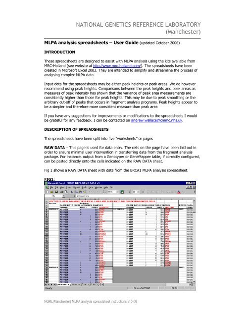
RAW DATA – This page is used for data entry. The cells on the page have been laid out in 

order to ensure minimal user intervention in transferring data from the fragment analysis 

package. For instance, output from a Genotyper or GeneMapper table, if correctly configured, 

can be pasted directly onto the cells indicated on the RAW DATA sheet. 

Fig 1 shows a RAW DATA sheet with data from the BRCA1 MLPA analysis spreadsheet. 

FIG1: 

NGRL(Manchester) MLPA analysis spreadsheet instructions v10-06

RESULTS – as the title suggests this page displays the results of the analysis. The results 

from the test samples are analysed in comparison with a group of 5 normal controls (see the 

analysis section for a more detailed description of the method of analysis). The results are 

displayed in four principal ways (i) as dosage quotients (DQs) gridded for each ligation 

product versus each control ligation product (ii) graphically as mean dosage quotient for each 

ligation product (iii) as a likelihood probability and odds for each ligation product calculated 

for one of three hypotheses – that the dosage is normal (2n copies), that the dosage is 

deleted (n copies) or that the dosage is duplicated (3n copies). 

Fig 2 shows the RESULTS sheet for some typical data entered into the BRCA1 MLPA 

spreadsheet. 

FIG2: 

CALC1 – this sheet is simply used for calculation. The dosage data is first normalised on this 

sheet depending on the signal strength of the control amplimers. The deviations of each test 

sample ligation product are also calculated on this sheet relative to the mean and standard 

deviation of the 5 normal controls. 

CALC2 – this sheet is also used for calculation. On this sheet the peak heights of each 

ligation product are divided by every other peak height within a sample to yield a ratio. This 

is then divided by the equivalent figure derived from the average of the five normal controls 

to yield the dosage quotients displayed on the RESULTS worksheet. 

REGRESSIONS – this sheet is used to correct for any data that slopes relative to increasing 

molecular weight of the product. We have found artefacts in data causing slope due to 

differences in the electrokinetic injection sample loading process used in capillary 

electrophoresis. Data is normalised on this page using a linear regression model based on the 

degree of sloping of the control ligation products. In kits where there are no clear control 

ligation products e.g. Human Telomere MLPA kits P069/P070, then all ligation products are 

used in the calculation of slope. 


METHOD OF ANALYSIS 

Background 

Analysis of dosage data can be problematic. Dosage data is quantitative yet in diagnostics we 

require a binary (Yes or No) answer. Analysis of dosage data by the use of dosage quotients 

(DQs) has been generally accepted as the standard method of analysis for several years. 

These worksheets analyse data to produce DQs in the standard way; however, they also 

incorporate two novel features of analysis to aid with interpretation. 

The first generates a likelihood probability of concordance with one of three hypotheses. 

Namely that a ligation product is present at either one two or three copies within the test 

sample. This figure is generated by comparing the test sample to a series of five normal 

controls. The controls are used to give a measure of the variability for each ligation product 

and allows the probability of deviation from expectation of the test sample to be estimated 

using the t-statistic. 

The second acts as a control for the overall quality of an individual test by measuring the 

standard deviation of the DQs obtained for all the control ligation products. If the standard 

deviation exceeds 0.1 then the sample is deemed to be of poor quality. Studies carried out by 

Dr Ruth Charlton, Regional Genetics Service, Leeds have shown that there is no overlap 

between DQs of deleted, normal and duplicated DQs of samples where the standard deviation 

of the control ligation products do not exceed 0.1. Thus excluding samples with higher 

degrees of variability substantially reduces the possibility of making an incorrect diagnosis. 

The analysis process 

Firstly the data is input on the RAW DATA worksheet. The format of this sheet has been to 

designed to facilitate the input of data directly from fragment analysis applications with the 

minimum user intervention e.g. Genotyper/Genemapper. This data is then presented in a 

more amenable format either at the top or bottom of the RESULTS worksheet. 

Each test and control sample’s data is normalised by summing the total control peak height 

and dividing each ligation product’s peak height by this figure. Carrying out this step is 

necessary in order for meaningful measurements of the variability between control samples to 

be measured. The control and test data is then ‘equalised’ by dividing the normalised peak 

height by the mean peak height of all five controls. Both these stages are carried out on the 

CALC1 sheet. 

The next step that is carried out is to correct for ‘sloping’. This is achieved by carrying out a 

linear regression of all the equalised control products (or all equalised products if there are no 

control products) against the mean of the five control samples and correcting the equalised 

peak heights for the slope of any regression calculated according to the molecular weight of 

each peak. This stage is carried out on the REGRESSIONS sheet. 

Dosage quotients (DQs) are next calculated firstly by dividing each slope corrected ligation 

product peak height by each slope corrected control ligation product peak height for the 

average of all five control samples to create a matrix or grid of values. The same set of 

calculations are carried out for each of the test samples. These matrices are displayed on the 

CALC2 sheet. The dosage quotients are then calculated by dividing the test sample matrix by 

the control mean matrix. Dosage quotients (DQs) are displayed on the RESULTS sheet. 

The mean and standard deviation of each ligation product is then calculated for the five 

normal controls. 

The fit to each of the three hypotheses (deleted, normal or duplicated) is then calculated as 

follows. For the normal (2n copies) hypothesis, the difference of each test sample’s ligation 

product normalised peak height from the mean of the control samples is calculated as a 

number of standard deviations. For the deleted hypothesis (n copies) the assumption is made 

that if the test sample is heterozygously deleted for a ligation product that the peak should 


e half-height and thus doubling the normalised peak height should therefore yield good fit 

with the control data. Thus doubled normalised peak heights are compared with the 

corresponding mean control amplimers to yield a difference as numbers of standard 

deviations for the deleted hypothesis. Finally, to test fit to the duplicated (3n) hypothesis the 

assumption is that if duplicated the test sample should be 1.5 times normal height thus 

multiplying the test sample normalised peak height by 2/3 should yield good fit with the 

control data. 

The three differences representing the three competing hypotheses are then converted into 

probabilities of deviation using the t-statistic. The precise probability for each amplimer is 

thus determined by two factors (i) the underlying variability in the batch of five normal 

controls for that particular ligation product and (ii) the size of the difference between the test 

sample for that ligation product and the control samples. 

Finally the relative likelihood of each of the three competing hypotheses is calculated for each 

ligation product as an odds ratio to indicate which hypothesis is more likely. For instance if 

the observed deviation from the normal hypothesis of the test sample is predicted to occur in 

10% cases and the deviation from the deleted hypothesis is predicted to occur in 0.1% of 

cases then the relative odds of the normal to deleted hypotheses is 100:1 in favour of the 

normal hypothesis. 

Fig 3 illustrates the method used for calculating relative likelihoods. The three curves 

represent the relative probability distribution of dosage quotient for a given ligation product 

for each of the hypotheses, n – deleted, 2n – normal, 3n – duplicated. The probability 

distribution is calculated in practice by the t-statistic. In the illustrated example the measured 

DQ of 0.9 equates to a probability of this being a normal result of 0.40, a probability of being 

a deleted result of 0.0009 and a probability of being a duplicated result of 0.0006. Dividing 

the Normal probability by the Deleted probability yields an odds ratio of 444:1 and dividing 

the Normal by the Duplicated probability yields an odds ratio of 667:1. 

Fig 3: 

p 

n 2n 3n 

DQ 

0.5 1.0 1.5 

DQ = 0.9; p(2n) = 0.40 

p(n) = 0.0009; p(3n) = 0.0006 

Odds Norm:Del = 444:1 

Odds Norm:Dup = 667:1 

USE OF AND INTERPRETATION OF DATA ON THE WORKSHEETS 

The spreadsheet may be started by simply opening the file in Excel or double clicking the file 

icon in Windows Explorer. Depending on the levels of Macro Security set on your workstation 

you may or may not be informed that the spreadsheet contains macros and given the 

opportunity to enable or disable them but if macros are enabled a small dialog box is 

presented to the user (see Fig 4). The user must then enter both their name and 

corresponding laboratory worksheet number in order to proceed with analysis. The user name 

and Worksheet number are then entered on the worksheet within locked cells for audit 

purposes. This feature can be bypassed if preferred as some spreadsheets still function 

normally with macros disabled, however it is important to note that some do not e.g. P069 

and P070 Human Telomeres. Any spreadsheets where macros need to be enabled in order for 

the spreadsheet to function normally will state this in the Release Notes. Should you need to 


change the Macro security setting to allow macros to run, this can be done as follows in MS 

Excel 2003 

FIG 4: 

• On the Tools menu, click Options. 

• Click the Security tab. 

• Under Macro Security, click Macro Security. 

• Click the Security Level tab, and then select the security level you want to use – 

Medium is recommended, 

Data may now be copied and pasted directly from a Genotyper or equivalent output table in 

Excel format onto the RAW DATA sheet. The yellow cells indicate the cell(s) to select when 

pasting data. 

Fig 5 illustrates the appearance of the RAW DATA sheet prior to entering data. 

FIG 5: 

The spreadsheets must have five normal controls in order to function correctly. Once data 

has been pasted into position the “Cross Ref” column can be used to ensure that the data has 

been pasted into the sheet in the correct order provided the pasted data also includes data 

labels. 


Fig 6 illustrates some data showing the concordance between the LABEL 1 field from the 

pasted data and the “CROSS REF” field. 

FIG 6: 

Space is allocated for a deletion or positive mutation control. Although this is not essential for 

the spreadsheet to function properly we strongly recommend that at least one positive 

control is run with each batch of samples. The data entry form is configured to accept up to 

10 test samples. 

Once the test samples have been entered onto the RAW DATA sheet the results may be 

visualised by clicking on the RESULTS tab. 

On the RESULTS sheet, the control and test sample raw data are represented at the top of 

the sheet. Further down the sheet the analysed data are presented with the deletion control 

displayed first followed by up to 10 test samples. To the left of each sample’s analysed data 

is a set of cells in which the sample name/lab no (from the raw data sheet), user and 

worksheet number (as entered in the dialog box when the worksheet was opened) is 

displayed for record keeping purposes. Beneath the worksheet information is a cell labelled 

“Int QC Stand Dev”. The cell directly below will either be coloured green if the sample quality 

is judged as good or red if it is judged poor. Sample quality is estimated by measuring the 

standard deviation of all the test ligation products measured against each other. As outlined 

previously retrospective analysis of MLPA data has shown that samples with control standard 

deviations less than 0.1 show no overlap between normal, duplicated and deleted ranges (Dr 

Ruth Charlton). 

Fig 7a illustrates the appearance of a typical sample where the data quality has been judged 

to be poor. 

FIG 7a: 

In worksheets where there are no control ligation products e.g. P069 and P070 Human 

telomeres, any cells that have been excluded from the quality control calculation due to them 

being possibly deleted or duplicated are listed in the cell below the data quality cell. If no 

cells have been excluded i.e. none have been judged as potentially deleted/duplicated the 

text ‘Omitted;None’ appears. 


FIG 7b: 

To the right of this sample information, the results are presented in a tabular format. For 

each sample, the upper rows are a series of dosage quotients gridded out for each ligation 

product (control and test) horizontally versus each control ligation product vertically. These 

cells are conditionally formatted to highlight deleted/duplicated and aberrant results. The 

actual settings that have been set for the conditional formats are given to the right of the raw 

data and may vary depending on the spreadsheet but typical ranges are as follows: 

Normal DQ 0.85 – 1.15 

Deleted DQ 0.35 – 0.65 

Duplicated DQ 1.35 – 1.65 

Equivocal DQ 0.65-0.85 & 1.15-1.35 

Fig 8 illustrates a test sample showing a section of DQ results from a sample. The majority of 

DQs fall into the normal range and have a white background. A patch of three ligation 

products (BRCA1 Exons 1A, 1B and 2) all have reduced DQs within the deleted range of 0.35- 

0.65 and are shaded aqua (ringed). A single DQ measurement, that between the control 

ligation product C11p13 and C12p12 lies in the “equivocal” range and is shaded a cream 

colour. 

Fig 8: 

Beneath the gridded DQ data lie (typically) two rows labelled in blue type above three rows 

labelled in green type. These rows hold the probabilistic analysis of the sample’s mean DQ 

result for each ligation product. The green rows contain absolute probabilities measured by 

the t-statistic of the difference between the observed mean DQ for that ligation product and 

the expected DQ as estimated from the panel of 5 normal controls for each of the possible 

dosages (normal, deleted and duplicated). A 60% probability in the row for the normal 

hypothesis indicates that a random normal sample would be expected to deviate by at least 

this amount in 60% of tests. These cells are also conditionally formatted to highlight 

abnormal or equivocal results. The precise limits may vary from spreadsheet to spreadsheet 

but a key is given to the right of the control data at the top of the RESULTS sheet. 

The blue rows contain pairwise comparisons between the relative probabilities for the 

alternative hypotheses given as an odds ratio. With good quality data the odds ratios 

although varying should clearly favour one hypothesis over another. If the “normal” i.e. 2n 

hypothesis is clearly favoured (i.e. an odds ratio of >=20:1 for normal) the cell is 

conditionally formatted to have a green background. A clear odds ratio in favour of an 

abnormal hypothesis (i.e. an odds ration of >=1:20 in favour of a deleted or duplicated 

hypothesis) gives a cell with a red background. Any odds ratio giving equivocal results is 

highlighted with a cream background. 


Figure 9 illustrates some typical results. Most of the odds ratios for the shown ligation 

products strongly favour the normal hypothesis and are consequently shaded in with a green 

backround. However the ligation product for BRCA1 Ex 13 is showing high DQs, consequently 

the fit is better to the duplicated hypothesis than either the normal or deleted hypotheses. 

Comparing the relative probabilities of fit to the duplicated and normal hypotheses the 

relative likelihood is calculated as 146:1 in favour of the sample being duplicated than the 

result being a normal outlier experienced by chance. 

Fig 9: 

The spreadsheets also incorporate a graphical representation of the results in the form of a 

histogram. This is located to the right of each test sample on the RESULTS sheet. 

Fig 10 illustrates a histogram from the HNPCC MLPA spreadsheet summarising the mean DQ 

data. This particular sample gave normal odds ratios for all ligation products except that for 

hMLH1 exon 2 which appeared to be deleted. This was subsequently confirmed by further 

analysis. 

FIG 10: 

INTERNAL QUALITY CONTROL 

Internal quality control is an important consideration for all diagnostic laboratories. Although 

the extra tiers of analysis given in the spreadsheets assist in the analysis of MLPA dosage 

data, the meaning and significance of some results will still remain a matter of professional 

judgement. The precise limits of what is an acceptable result must remain the responsibility 

of each laboratory to determine, however what follows are guidelines that have been found 

to be useful locally. 

1) In order to be an acceptable result the “Quality” value (standard deviation of the control 

ligation products) should have a value of = 20:1 odds then the sample can 

be judged to be normal. 

3) If two or more contiguous ligation products favour a deleted or duplicated hypothesis with 

>= 1:20 odds then the sample can be judged to be abnormal provided the remaining ligation 

products give odds ratios for the normal hypothesis of >= 20:1 odds. It still remains good 


practice to confirm any mutations by repeating the analysis on a replicate MLPA analysis or 

on an affected first degree relative 

4) If a single ligation product gives a >= 1:20 odds ratio in favour of deletion/duplication 

then further evidence must be obtained to confirm this result. Firstly the sample should be 

sequenced to establish that there are no mutations present beneath the ligation product 

hybridisation sites (this has been a frequently cause of a ligation product which appears 

deleted). Secondly the deletion/duplication should either (i) be confirmed using a separate 

assay e.g. long PCR, dosage PCR (ii) be confirmed on a separate DNA sample (not just a new 

replicate MLPA assay) or (iii) be confirmed on an affected first degree relative. 

5) Where a sample otherwise appears normal yet the odds ratios for normality drop below 

>= 20:1 for some test ligation products this can be accepted to be a normal result provided 

(i) no one normal odds ratio drops below 5:1 in favour of normality (ii) that contiguous exons 

are not involved (iii) that no more than 10% of test ligation products are involved (iv) that 

none of the mean DQs falls into the transitional range (0.7-0.8 or 1.2-1.3). Please note that in 

the presence of a deletion the normal:duplication comparison is meaningless and will yield 

equivocal odds the same applies for the normal:deletion comparison for a duplicated sample. 

SPREADSHEETS FOR NEW MLPA ASSAYS 

If there is an MLPA assay in use in your laboratory for which you would like us to design a 

spreadsheet please contact me by email at andrew.wallace@cmmc.nhs.uk 

CONFIGURATION OF EXISTING SPREADSHEETS 

If there is an existing spreadsheet for which the data entry page is not compatible with your 

fragment analysis output, I can usually quite simply alter these to suit your requirements. In 

order to do this please email to me at andrew.wallace@cmmc.nhs.uk a sample of your data 

which you would like to import directly into the spreadsheets 

MODIFICATIONS TO EXISTING PROBE SETS 

MRC-Holland review their kits and often change the probe combinations in response to their 

customer demand. If you notice that this has occurred and the currently available 

spreadsheet will no longer analyse the data please let me know by email at 

andrew.wallace@cmmc.nhs.uk as I can usually make minor modifications quite easily. 

ACKNOWLEDGEMENTS 

The quality control measure using the standard deviation of the control ligation products was 

developed by Dr Ruth Charlton, Regional Genetics Service, Leeds

Manchester - National Genetics Reference Laboratories

Create successful ePaper yourself

Delete template?

Save as template?