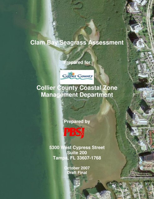
Clam Bay Seagrass Assessment Collier County Coastal Zone ...

Clam Bay Seagrass Assessment
Prepared for
Collier County Coastal Zone
Management Department
Prepared by
5300 West Cypress Street
Suite 200
Tampa, FL 33607-1768
October 2007
Draft Final

Table of Contents
Table of Contents.......................................................................................................................................... i
1.0 Introduction .....................................................................................................................................1
1.1 Development of Clam Bay .................................................................................................1
1.2 Seagrass Mapping .............................................................................................................3
2.0 Methods ..........................................................................................................................................7
2.1 Task 1 – Kickoff Meeting and Stakeholder Interviews .......................................................7
2.2 Task 2 – Data Collection on Depth Distribution of Seagrasses and Potential
Water Clarity Goals for Clam Bay......................................................................................7
2.2.1 Seagrass Sampling...............................................................................................7
2.2.2 Water Quality Sampling ........................................................................................8
2.3 Task 3 – Development of Estimated Freshwater and Pollutant Loading Estimates
for the Clam Bay Watershed..............................................................................................9
2.3.1 Model Development ..............................................................................................9
2.3.2 Major Watersheds...............................................................................................11
3.0 Results ..........................................................................................................................................16
3.1 Seagrass distribution........................................................................................................16
3.2 Water Quality ...................................................................................................................23
3.2.1 Based on the data collected, what were the general water quality
conditions in Clam Bay during our study? ..........................................................25
3.2.2 What water quality parameters (i.e., turbidity, phytoplankton, and “color”)
best explain differences in water clarity? ............................................................25
3.2.3 Which nutrient, nitrogen or phosphorus, best explains differences in
phytoplankton abundance?.................................................................................26
3.2.4 Are our conclusions in-line with prior assessments of water quality in
Clam Bay?...........................................................................................................28
3.3 Pollutant Loading Model ..................................................................................................31
3.3.1 Net Pollutant Loads.............................................................................................33
4.0 Conclusions and Action Plan ........................................................................................................36
5.0 References....................................................................................................................................40
i Clam Bay Seagrass Assessment
DRAFT October 2007

Contents
List of Figures
Figure 1.1 Aerial Photo (circa 1940s) of Clam Bay and immediate watershed .................... 1
Figure 1.2 Aerial photograph (2006) of Clam Bay and immediate watershed...................... 2
Figure 1.3 Spatial extent of seagrass meadows (dotted areas) as reported in the
Collier County Seagrass Protection Plan (1992).................................................. 4
Figure 1.4 Spatial extent of seagrass meadows (striped areas) as reported by Collier
County Seagrass Inventory (1994). ...................................................................... 5
Figure 2.1 Pollutant Loading Flow Chart ............................................................................ 10
Figure 2.2 Overview of Clam Bay, with sub-basin boundaries used for the pollutant
loading model. ..................................................................................... 11
Figure 3.1 Potential sample sites in Clam Bay .................................................................... 16
Figure 3.2 Presence (green) and absence (red) of seagrass from visited sample sites
in Clam Bay. ..................................................................................... 17
Figure 3.3 Location of “reference sites” within the Dollar Bay / Gordon Pass areas. ........ 19
Figure 3.4 Seagrass presence in two “reference sites”. ....................................................... 20
Figure 3.5 Seagrass (green) and oyster (pink) coverage in southern Naples Bay in
1953 (image from City of Naples). .................................................................... 21
Figure 3.6 1952 aerial photograph of Clam Bay (from Antonini et al. 2002)..................... 22
Figure 3.7 Locations of visited water quality stations. ........................................................ 23
Figure 3.8 Water clarity (Secchi disk depth) vs. turbidity (NTU) for all stations
combined for Clam Bay. .................................................................................... 26
Figure 3.9 Chlorophyll-a vs. total nitrogen for all stations combined for Clam Bay. ......... 27
Figure 3.10 Chlorophyll-a vs. total phosphorus for all stations combined for Clam
Bay. ..................................................................................... 27
Figure 3.11 Comparison of average TN concentrations for this study (blue bars) to
previous data (green bars). ................................................................................. 29
Figure 3.12 Comparison of average TP concentrations for this study (blue bars) to
previous data (green bars). ................................................................................. 29
Figure 3.13 Total dissolved solids over the period of record at station W-1. Solid line
is moving 10-point average. ............................................................................... 30
Figure 3.14 Total nitrogen over the period of record at station W-1. Solid line is
moving 10-point average.................................................................................... 30
Figure 3.15 Total phosphorus over the period of record at station W-1. Solid line is
moving 10-point average.................................................................................... 31
ii
Clam Bay Seagrass Assessment
DRAFT October 2007

Contents
List of Tables
Table 2.1 Braun-Blanquet seagrass coverage method.......................................................... 8
Table 2.2 Sampled water quality parameters for Clam Bay sites......................................... 9
Table 2.3 Current and historic land use / land cover by category for the Clam
Bay watershed. ..................................................................................... 12
Table 2.4 EMC values for total nitrogen, total phosphorus, and total suspended
solids (values in mg / liter). ................................................................................ 14
Table 2.5 BMP Removal Efficiencies (TSS, TN, TP)........................................................ 15
Table 3.1 Water quality results for selected parameters for 5 stations in Clam
Bay. Data are means of n = 6. “Fla. Median” = median value for
Florida Estuaries. “Fla. 10% Best” is value below which are the best
10% of estuary values. “Fla. 10% Worst” is value above which are
worst 10% of estuary values. “NA” = not available.......................................... 24
Table 3.2 Total dissolved solids (TDS), TN and TP from station W-1.............................. 28
Table 3.3 Historic and current conditions runoff (acre-feet / yr) by subbasin. .................. 32
Table 3.4 Gross Historic, Gross Current, and Net Current TN loads (pounds / per
year) for Clam Bay subbasins. ........................................................................... 33
Table 3.5 Gross Historic, Gross Current, and Net Current TP loads (pounds / per
year) for Clam Bay subbasins. ........................................................................... 34
Table 3.6 Gross Historic, Gross Current, and Net Current TSS loads (pounds /
per year) for Clam Bay subbasins. ..................................................................... 35
iii
Clam Bay Seagrass Assessment
DRAFT October 2007

1.0 Introduction
1.1 Development of Clam Bay
Clam Bay is an important natural feature in Collier County. Recent reports have indicated that
Clam Bay is experiencing losses in seagrass coverage, which has led to concern among the
public that one of the more picturesque natural features of western Collier County is in danger of
being seriously degraded.
The Clam Bay watershed, like much of Collier County, has experienced dramatic changes over
the past 60 years. In the 1940’s, there was little evidence of human modifications to Clam Bay
and its immediate watershed (Figure 1.1).
Figure 1.1– Aerial Photo (circa 1940s) of Clam Bay and immediate watershed
In contrast, more recent aerial photography clearly shows modifications to both the Clam Bay
shoreline and the dramatic changes in the watershed (Figure 1.2).
1 Clam Bay Seagrass Assessment
DRAFT October 2007

Introduction
Figure 1.2 – Aerial photograph (2006) of Clam Bay and immediate watershed
Modifications to the Clam Bay system include the construction, in 1958, of Seagate Drive, which
severed the previous tidal connection between Clam Pass (to the north) and Doctors Pass (to the
south). A series of culverts were put in place in 1976 to alleviate this condition, but it appears
that their effectiveness was perhaps minimal, and upgraded features were necessary for them to
increase flushing properly (Antonini et al. 2002). Recent decades have also been characterized
by the rapid urbanization of the Clam Bay watershed. Prior studies in similar lagoonal systems
in Southwest Florida suggest that increased urbanization brings about increased freshwater
inflows and substantial increases in nonpoint sources of both nitrogen and phosphorus (i.e.,
Lemon Bay - Tomasko et al., 2001).
In the early 1990s, an area of mangrove die-off of approximately seven acres was discovered in
Upper Clam Bay, north of Clam Pass. By the mid-1990s, the area of die off (affecting mostly
black mangroves) had expanded to approximately 50 acres. In response to the die-off, Pelican
Bay residents acquired the services of a series of consultants to develop a plan of action to
remediate the mangrove loss. In the meantime, various intermediate measures were performed,
including the dredging of Clam Pass in April of 1996 and the clearing of several channels by
hand evacuation in August and November of 1996 (Conservancy of Southwest Florida 1997).
2 Clam Bay Seagrass Assessment
DRAFT October 2007

Introduction
Based on assessments of water quality data collected by Collier County Environmental Services
and the Pelican Bay Services District, there did not appear to be evidence that mangrove
mortality was caused by elevated levels of any toxic chemicals, nor did the data suggest changes
in nutrient concentrations would have been a likely factor in die-off. Instead, the conclusion was
reached that die-off was likely due to excessive freshwater input to the system from the adjacent
developed uplands and an inadequate dispersion of the increased freshwater input due to severely
constricted tidal channels in the mangrove forest. As a result, the mangrove forest became
inundated with water levels higher than the tops of the black mangrove pneumatophores. The
duration of increased water levels was sufficient to kill the tress by blocking oxygen exchange to
the below ground tissues. In 1998, the Collier County-Pelican Bay Services Division was issued
a permit to restore and manage the Clam Bay Natural Resource Protection Area based on the
Clam Bay Restoration and Management Plan (Brown and Hillestad 1998).
The management component of the Clam Bay Restoration and Management Plan consists of four
major activities:
1. Retrofitting of the culverts under Seagate Drive with flap gates, such that flow only goes
north.
2. Redredging of Clam Pass.
3. Excavation of tidal connections in interior portions of Upper Clam Bay.
4. Development of stormwater best management plans for on-site retention of water from
surrounding development.
1.2 Seagrass Mapping
Existing results from ongoing seagrass mapping efforts in Clam Bay (T. Hall, personal
communication) suggest that coverage of this important habitat had declined between 1994 and
2006. It has also been suggested that a more precipitous decline in coverage occurred between
1991 and 1994. The reported seagrass decline in the early 1990s is mostly attributed to results
listed in two mapping projects, both conducted by Collier County.
In the first report, the Collier County Seagrass Protection Plan (1992) concluded that seagrass
coverage in Clam Bay was equivalent to approximately 60 acres, and that “Outer Clam Bay
contains one of the densest and most extensive seagrass beds in the County.” The spatial
coverage of seagrass meadows, as reported in the 1992 Seagrass Protection Plan is shown in
Figure 1.3.
3 Clam Bay Seagrass Assessment
DRAFT October 2007

Introduction
Figure 1.3 – Spatial extent of seagrass meadows (dotted areas) as reported in the
Collier County Seagrass Protection Plan (1992).
In a later report, Collier County Seagrass Inventory (1994) mapped seagrass coverage in Clam
Bay, and estimated that approximately 10 acres of seagrass were present in the same area (Figure
1.4).
4 Clam Bay Seagrass Assessment
DRAFT October 2007

Introduction
Figure 1.4 – Spatial extent of seagrass meadows (striped areas) as reported by
Collier County Seagrass Inventory (1994).
If the mapped seagrass coverage estimates from these two reports were accurately reporting the
true acreage of seagrass meadows, a decrease in coverage of more than 80 percent occurred in
the early 1990s. This would be a more precipitous decline than was documented for Tampa Bay
during the time period of the 1950s to the early 1980s (Tomasko 2002).
In response to these concerns, the Clam Bay Working Group contacted PBS&J to conduct a
study to determine the following:
• What is the extent of seagrass resources in Clam Bay?
• How has seagrass coverage changed over the recent past?
• What are the most likely factors associated with recent declines?
• How have freshwater inflow and nutrient loads to Clam Bay changed over time?
• What actions might reasonably be expected to allow for recovery of these seagrass
resources?
5 Clam Bay Seagrass Assessment
DRAFT October 2007

Introduction
• What would be a reasonable timeline and budget for implementing such a recovery plan?
To answer these questions, PBS&J completed the following tasks: 1) conduct a kickoff meeting
for the project, and interview interested stakeholders, 2) collect water quality and seagrass data
from within Clam Bay, 3) develop a pollutant loading model for Clam Bay, and 4) develop an
“Action Plan” to address any identified environmental stressors to Clam Bay.
6 Clam Bay Seagrass Assessment
DRAFT October 2007

2.0 Methods
2.1 Task 1 – Kickoff Meeting and Stakeholder Interviews
The PBS&J project team met with staff from Collier County to conduct detailed interviews with
the following stakeholders and/or sources of information:
• Dave Busier – Seagate
• Tim Hall – Turrell and Associates
• John Domenie – PBSD
• Kyle Lukasz - PBSD
• Jim Burke – PBSD
• Kathy Worley – the Conservancy of Southwest Florida
• Others as identified by Collier County
In addition, PBS&J reviewed the following information and data sets:
• All detailed monitoring reports and testing results performed by Pelican Bay Services
Division and /or their consultants.
• Collier County aerial photographs
• Any and all seagrass data from Clam Bay
• Annual reports and raw data collected from Turrell and Associates
• Conversancy of SW Florida water quality data on Clam Bay
2.2 Task 2 – Data Collection on Depth Distribution of Seagrasses and Potential
Water Clarity Goals for Clam Bay
2.2.1 Seagrass Sampling
The techniques used in this report involved the following steps: 1) identification of seagrass
extent in Clam Bay, 2) identification of seagrass in two reference bays, 3) collection of water
quality data in Clam Bay, 4) determining those factor(s) responsible for variation in water clarity
in Clam Bay, and 5) determining the nutrient most likely to be limiting phytoplankton growth in
Clam Bay.
Using an ArcGIS Random Number Generator tool within a GIS-generated polygon for Clam
Bay, a sampling “universe” of 100 potential sampling sites was generated. Of those 100
potential sites, 30 were chosen at random for groundtruthing for seagrass coverage. Each of the
thirty sampling points was located using a WAAS (Wide Area Augmentation System) enabled
Garmin GPSmap 60CSx. A modified Braun-Blanquet method was used to determine seagrass
coverage (Table 2.1). Three assessments of seagrass coverage and species diversity were
recorded for each of the 30 visited sites, using a 1m 2 quadrant in May 2007. The water depth,
substrate (muddy, sandy, etc.) and presence/absence of macroalgae were also recorded.
7 Clam Bay Seagrass Assessment
DRAFT October 2007

Methods
Table 2.1- Braun-Blanquet seagrass coverage method.
Assessed Value Percent Seagrass Coverage
0 No coverage
0.1 Solitary short shoot
0.5 Sparse of

Methods
Table 2.2 - Sampled water quality parameters for Clam Bay sites.
Physical
pH
Parameter Unit Method
Standard
units
YSI
Temperature °C YSI
Dissolved Oxygen (DO) mg/l YSI
Specific Conductivity µmhos/l YSI
Secchi Depth cm Secchi Disk/ measuring tape
Turbidity NTU SM 18 2130 B
Color Pt-Co 110.2
Total Suspended Solids (TSS) mg/l 160.2
Volatile Suspended Solids (VSS) mg/l 160.2
Chemical
Total Kjeldahl (TKN) mg/l SM20 4500-Norg D
Total Phosphorus (TP) mg/l SM18 4500-P E (P
Nitrate+Nitrite (NOx) mg/l EPA 353.2
Ortho-Phosphate (SRP) mg/l SM18 4500- P E
Total Phosphorus (TP)
Biological
mg/l
Chlorophyll a (Chl a) µg/l SM18 10200H
Finally, the water quality data sets collected within Clam Bay by the Conservancy of Southwest
Florida and the Pelican Bay Services Division were reviewed and analyzed, if found appropriate,
to examine trends in nutrients, salinity, etc. within Clam Bay.
2.3 Task 3 – Development of Estimated Freshwater and Pollutant Loading
Estimates for the Clam Bay Watershed
2.3.1 Model Development
An approach used by regulatory agencies in Florida estimates the average annual pollutant load
to quantify the amount of nonpoint source pollutants from surface waters discharged into a
waterbody. Calculations were conducted using the PBS&J Pollutant Loading Model. This model
is a GIS-based Pollutant Loading and Removal Model that uses data on hydrologic
characteristics, drainage characteristics, average annual rainfall, hydrologic parameters and
pollutant event mean concentrations (EMC).
Developing estimates of pollutant loads requires estimating both the stormwater runoff volume
and the corresponding concentration of the pollutants under consideration. Following the flow
chart seen in Figure 2.1 and described below, the Pollutant Loading Model incorporates, Soils,
Land Use, and Best Management Practices (BMP) GIS layers with Rainfall, Runoff, EMC, and
BMP efficiency lookup tables to calculate runoff volumes, gross loads, and net loads.
9 Clam Bay Seagrass Assessment
DRAFT October 2007

Methods
• Calculation of stormwater runoff volume. The runoff volume from a subbasin is
calculated as the product of the average, annual or seasonal, rainfall amount and the
subbasin’s weighted land use and soils rainfall / runoff coefficient. GIS coverages of land
use and hydrologic soil characteristics were intersected with subbasin delineations to
determine the area’s hydrologic characteristics.
• Calculation of gross pollutant loads. Gross pollutant loads are defined as the amount of
pollutant that is generated within a subbasin. This load is calculated as the sum of the nonpoint
source loads. The non-point source load is defined as the product of the estimated
annual runoff volume times the stormwater EMC for each selected pollutant and land use
category.
• Calculation of net pollutant loads. Net pollutant loads are defined as the amount of a
pollutant from a subbasin that is discharged into a receiving waterbody. This load is
calculated as the product of the gross pollutant load times a factor that represents the
estimated pollutant removal due to the occurrence of stormwater treatment within each
subbasin.
Figure 2.1 - Pollutant Loading Flow Chart
10 Clam Bay Seagrass Assessment
DRAFT October 2007

Methods
2.3.2 Major Watersheds
When the pollutant loading model is run, it generates contributions of runoff and loads for each
intersected polygon of soils, land use, and BMP. The sub-basin boundaries used for this analysis
are shown below in Figure 2.2.
Figure 2.2 – Overview of Clam Bay, with sub-basin boundaries used for the
pollutant loading model.
Land Uses
The Clam Bay watershed, as shown above, drains approximately 5,824 acres of highly urbanized
area. The present day land uses are compared to historical (1940’s) land use characteristics in
Table 2.3.
11 Clam Bay Seagrass Assessment
DRAFT October 2007

Methods
Table 2.3 – Current and historic land use / land cover by category for the Clam
Bay watershed.
Land Use / Land Cover
Current
Area
(acres)
Golf Course 310
High Density Residential 1,125
Historic Area
(acres)
High Intensity Commercial 433
Industrial 12
Low Intensity Commercial 248
Multi-Family Residential 918
Open Space 194 184
Road / Highway 146
Single Family Residential 1,351
Utility 13
Water 645 323
Wetlands 429 101
Mangrove 1,206
Mesic Flatwood 2,554
Xeric Hammock 1,457
Total 5,824 5,824
Historically, the dominant features of the Clam Bay watershed were the mixed vegetative
communities of mesic flatwoods and xeric hammocks. Mesic flatwoods dominated the lower
lying, wetter areas along the shoreline, as well as interior portions. Xeric hammocks dominated
the higher areas along the coastal ridge, where much of the US Highway 41 road bed was laid
out.
Currently, the major land use type is that of single-family residential land use, along with highdensity
residential land use. These two categories, along with multi-family residential land uses,
comprise a total of 3,394 acres or 58 percent of the combined watershed and open water area.
Golf courses comprise 310 acres, less than the amount of open water itself (645 acres). The
current land use / land cover layers list mangrove coverage in the category of “wetlands” while
our assessment of historical land cover had them separately categorized. Therefore, the current
12 Clam Bay Seagrass Assessment
DRAFT October 2007

Methods
category of “wetlands” includes mangrove fringes as well. Wetland loss in the Clam Bay
watershed is thus from 1,307 acres historically to a present day level of 429 acres, a decline of 67
percent.
Soils
The hydrologic characteristics of soil can significantly influence the capability of a given
watershed to hold rainfall or produce surface runoff. Soils of the Clam Bay watershed are
classified as Types A, B, C, or D, according to the following criteria (Viessman et al., 1989):
• Type A soil (low runoff potential): Soils having high infiltration rates even if thoroughly
wetted and consisting chiefly of deep, well-drained to excessively drained sands or gravels.
These soils have a high rate of water transmission.
• Type B soil: Soils having moderate infiltration rates if thoroughly wetted and consisting
chiefly of moderately deep to deep, moderately well-drained to well-drained soils with
moderately fine to moderately coarse textures. These soils have a moderate rate of water
transmission.
• Type C soil: Soils having slow infiltration rates if thoroughly wetted and consisting chiefly
of soils with a layer that impedes the downward movement of water, or soils with
moderately fine to fine texture. These soils have a slow rate of water transmission.
• Type D soil (high runoff potential): Soils having very slow infiltration rates if thoroughly
wetted and consisting chiefly of clay soils with a high swelling potential, soils with a
permanent high water table, soils with a clay pan or clay layer at or near the surface, and
shallow soils over nearly impervious materials. These soils have a very slow rate of water
transmission.
By knowing land uses and soil types, runoff volumes are then generated for each parcel of land.
These runoff volumes vary depending upon both the land use and the characteristics of the
underlying soils. The runoff volumes are then matched with literature-derived event mean
concentrations (EMCs) for various stormwater constituents, which are functionally equivalent to
a flow-weighted concentration. Simply put, the EMC value for any given constituent (e.g., total
nitrogen (TN), total phosphorus(TP), and total suspended solids (TSS)) is the concentration that
would be required to account for expected loads, based on storm-event sampling.
The EMC values used for the Clam Bay loading model are shown in Table 2.4.
13 Clam Bay Seagrass Assessment
DRAFT October 2007

Methods
Table 2.4 – EMC values for total nitrogen, total phosphorus, and total suspended
solids (values in mg / liter).
LAND_USE TN TP TSS
Single Family
Residential
High Density
Residential
Multi-Family
Residential
Low Intensity
Commercial
High Intensity
Commercial
2.29 0.3 27
2.3 0.4 50
2.42 0.49 71.7
1.18 0.15 81
2.83 0.43 94.3
Industrial 1.79 0.31 93.9
Utility 1.79 0.31 77
Road / Highway 2.08 0.34 50.3
Golf Course 2.32 0.34 55.3
Mesic Flatwood 1.25 0.053 11.1
Open Space 1.25 0.053 11.1
Xeric Hammock 1.25 0.053 11.1
Mangrove 1.6 0.09 10.2
Wetlands 1.6 0.09 10.2
Water 1.25 0.11 3.1
The loads calculated by knowing land use, soil type, runoff coefficients and EMC values are then
further modified via the use of selected “best management practices” or BMPs. The expected
removal efficiencies of these BMPs are shown in Table 2.5.
14 Clam Bay Seagrass Assessment
DRAFT October 2007

Methods
Table 2.5 - BMP Removal Efficiencies (TSS, TN, TP).
BMP Category TSS TN TP
Wet Detention Pond 70% 35% 60%
Wet Pond Treatment
Train
85% 50% 65%
Rainfall
In the estimation of annual pollutant loads, daily rainfall amounts represent the basic building
block or the foundation for the entire process. Rainfall data is used to generate runoff
coefficients for different land uses in the watershed and applied as an average annual rainfall
amount to determine the annual runoff volumes entering a waterbody. For the purposes of this
project, daily precipitation data were obtained from weather stations located in the City of
Naples from both the South Florida Water Management District (SFWMD) DBHydro database
(my.sfwmd.gov) and Weather Underground (www.wunderground.com). Data spanned a 52 year
period of from 1955 to 2007. Using this data as a continuous series, runoff coefficients were
generated, as previously discussed, in addition to the identification of the historic average annual
rainfall amount of 53.0 inches per year.
15 Clam Bay Seagrass Assessment
DRAFT October 2007

3.0 Results
3.1 Seagrass distribution
Figure 3.1 illustrates the “universe” of 100 potential sample site locations for the seagrass
assessment. Of those 100 potential sites, 30 were chosen at random for seagrass assessment.
The results of those surveys are illustrated in Figure 3.2.
Figure 3.1 – Potential sample sites in Clam Bay
16 Clam Bay Seagrass Assessment
DRAFT October 2007

Results
Figure 3.2 – Presence (green) and absence (red) of seagrass from visited sample
sites in Clam Bay.
Of the 30 seagrass sampling sites visited, seagrass was found in 13 of them, for a rate of
occurrence of 43 percent. While it would be tempting to convert this to an acreage estimate, by
assuming that if 43 percent of randomly chosen stations were occupied by seagrass, then 43
percent of the 60 + acres of Clam Bay is covered with seagrass (i.e., 26 acres of seagrass) this
would be an incorrect approach to the issue of seagrass coverage estimates. Techniques such as
random point visitations and transect-based assessments are not appropriate for translation into
acreage estimates.
At the station close to the Gulf of Mexico (Station 2), within the westernmost portion of Clam
Pass, a sprig of turtle grass, Thalassia testudinum, was encountered. This lone plant may have
17 Clam Bay Seagrass Assessment
DRAFT October 2007

Results
been transported to the site by currents or some other mechanism, as there was no evidence of a
meadow at this location.
At all other locations, the only species encountered was paddle grass, Halophila decipiens. This
species, H. decipiens, is typically found in either deeper waters in the Gulf of Mexico (i.e. waters
in excess of 50 feet in depth) or in low clarity waters in shallower locations (Dawes et al. 1989).
Of the 25 stations located south of the boardwalk that crosses from the mainland to the barrier
island, paddle grass was found at 12 stations, or nearly half of the sites visited. At those
locations, the average Braun-Blanquet score for seagrass coverage was 1.8, equivalent to bottom
coverage of between 5 and 25 percent.
In addition to surveys of seagrass coverage within Clam Bay, an assessment was made of the
relative coverage of seagrasses within other locations that were close by, but did not have direct
and adjacent human alterations of their shoreline and watersheds. The locations of these
“reference sites” are shown in Figure 3.3.
18 Clam Bay Seagrass Assessment
DRAFT October 2007

Results
Figure 3.3 – Location of “reference sites” within the Dollar Bay / Gordon Pass
areas.
19 Clam Bay Seagrass Assessment
DRAFT October 2007

Results
The location referred to as “Dollar Bay” actually represents only a portion of Dollar Bay, along
the eastern shoreline just south of Gordon Pass. The location referred to as “Gordon Pass” refers
to a small unnamed embayment located along the southern shoreline of Gordon Pass. Results
from the seagrass surveys at these locations are shown in Figure 3.4.
Figure 3.4 – Seagrass presence in two “reference sites”.
At both sites, a WAAS-enabled GPS unit was used to track the location of a diver surveying the
bottom of these bays and when seagrass was encountered, those locations were “tagged” for their
locations. Along the eastern shoreline of upper Dollar Bay, oysters were commonly found, as
well as the seagrass species called shoal grass (Halodule wrightii). Abundance was patchy and
20 Clam Bay Seagrass Assessment
DRAFT October 2007

Results
coverage was never more than approximately 25 percent of the bottom. Within the small
embayment located along the southern shoreline of Gordon Pass, seagrass was only found in the
northern lobe of that feature. Within that outermost portion, the species turtle grass (T.
testudinum) and shoal grass (H. wrightii) were encountered. In those areas farther south, no
seagrass was encountered, even though the deepest depths seemed to be approximately 3 to 5
feet – depths where seagrass was found within Clam Bay.
The seagrass results from Clam Bay suggest that seagrass is not an uncommon feature, but that
the species found, Halophila decipiens, is not one that is likely to be seen with aerial
photography. This species is a rather diminutive organism that is unlikely to be a discernable
feature with aerial photography and subsequent photointerpretation which can lead to “false
negatives” for abundance. Additionally, macroalgae, which can be abundant in Clam Bay, can
give “false positive” for photointerpertation, suggesting seagrass coverage where there is none to
be found. Thus, the seagrass species found in Clam Bay is not a species that is conducive to
mapping via traditional techniques, such as those used for seagrass mapping purposes in Tampa
Bay, Sarasota Bay, Lemon Bay, and Charlotte Harbor (e.g., Tomasko et al. 2005). Surveys of
nearby locations without any obvious human impacts, particularly the small embayment south of
Gordon Pass, suggest that lush seagrass meadows are not a presumed feature to be found in
Collier County’s estuaries. When examining 1950s seagrass maps from southern Naples Bay
Figure 3.5, (from the City of Naples), seagrass coverage (in green) has been lost from areas north
of Gordon Pass, but seagrass coverage wasn’t distinguishable in the 1950s in either Dollar Bay
or the small embayment south of Gordon Pass.
Figure 3.5 – Seagrass (green) and oyster (pink) coverage in southern Naples Bay
in 1953 (image from City of Naples).
Combined, these data suggest that the extent of seagrass coverage presently found in Clam Bay
is not necessarily indicative of a distressed system. Also, these data call in to question the
validity of Clam Bay once having had 60 + acres of lush seagrass meadows, as was suggested to
be the case in the 1992 Collier County Seagrass Protection Plan. When examining 1952
21 Clam Bay Seagrass Assessment
DRAFT October 2007

Results
photography from Clam Bay (Figure 3.6) there is no distinctive seagrass signature in the open
waters of the bay in this earlier, less-impacted condition. However, there does appear to be a
darker signature indicative of seagrass coverage in the shallower areas along the shoreline.
Figure 3.6 – 1952 aerial photograph of Clam Bay (from Antonini et al. 2002).
Outer Clam Bay
22 Clam Bay Seagrass Assessment
DRAFT October 2007

Results
3.2 Water Quality
The locations of the water quality sites visited for this study are shown in Figure 3.7.
Figure 3.7 – Locations of visited water quality stations.
Station 5 was chosen to represent a “boundary condition” of sorts for the Clam Bay system. It
was located in an area that experiences much greater water exchange, where the cross sectional
area is reduced considerably and water movement has a much greater velocity than areas farther
south. Stations 27 and 26 were located on the western and eastern boundaries of the bay,
respectively, while station 14 was located in the middle of the bay. An additional station,
23 Clam Bay Seagrass Assessment
DRAFT October 2007

Results
“Canal” was located at the eastern end of an east-west oriented residential canal connected to
Clam Bay.
The water quality data were then analyzed for a number of different determinations. Among
these were the following:
1. Based on the data collected, what were the general water quality conditions in Clam Bay
during our study?
2. What water quality parameters (i.e., turbidity, phytoplankton, and “color”) best explain
differences in water clarity?
3. Which nutrient, nitrogen or phosphorus, best explains differences in phytoplankton
abundance?
4. Are our conclusions in-line with prior assessments of water quality in Clam Bay?
Water quality at the five sampled locations, during this study, is summarized in Table 3.1.
Table 3.1 – Water quality results for selected parameters for 5 stations in Clam
Bay. Data are means of n = 6. “Fla. Median” = median value for Florida Estuaries.
“Fla. 10% Best” is value below which are the best 10% of estuary values. “Fla.
10% Worst” is value above which are worst 10% of estuary values. “NA” = not
available.
Location
Salinity
(ppt)
Chl-A
(µg / liter)
Total
Nitrogen
(mg / liter)
Total
Phosphorus
(mg / liter
Turbidity
(NTU)
Color
(PCU)
CB-5 37.3 3.3 0.44 0.03 2.18 4.2
CB-14 36.3 4.4 0.40 0.04 2.53 4.6
CB-26 36.4 5.8 0.46 0.04 3.82 15.0
CB-27 35.9 9.2 0.50 0.05 4.83 10.4
CB-CNL 35.5 10.5 0.52 0.06 3.73 18.3
Fla. Median NA 9 0.8 0.07 NA NA
Fla. Best
10%
Fla Worst
10%
NA 1 0.3 0.01 NA NA
NA 36 1.6 0.20 NA NA
24 Clam Bay Seagrass Assessment
DRAFT October 2007

Results
3.2.1 Based on the data collected, what were the general water quality conditions
in Clam Bay during our study?
Salinities at all locations were high, indicating minimal freshwater influence during the time
period of May 16 to July 26 of 2007. Levels of chlorophyll-a, an indicator of algal biomass,
were lowest at the station closest to Clam Pass (CB-5) and highest at the canal site (CB-CNL).
At no locations did average values exceed the Florida Department of Environmental Protection’s
(FDEP) Impaired Waters Rule guidance criteria of 11 µg / liter, although the canal site came
close to being “impaired”. During this time, chlorophyll-a levels were mostly below or close to
the median value of chlorophyll for Florida estuaries.
Levels of total nitrogen (TN) were below the median value for Florida estuaries (0.8 mg TN /
liter), as derived by FDEP (1996). The TN level at CB-14 was only 50% of the median TN
value, while even the highest TN value, at CB-CNL, was still only 65% of the median value for
Florida estuaries.
Levels of total phosphorus (TP) were much lower than the median value of TP for Florida
estuaries (0.07 mg TP / liter; FDEP [1996]) at stations CB-5, CB-14 and CB-26. However,
values at station CB-CNL, in particular, were 86% of that median value.
3.2.2 What water quality parameters (i.e., turbidity, phytoplankton, and “color”)
best explain differences in water clarity?
To determine what water quality parameter best explained variation in water clarity, Secchi disk
depths were compared to those water quality parameters that had optical properties (i.e.,
chlorophyll-a, turbidity, color). Simple regressions were run with Secchi disk depth as the
dependent variable, and chlorophyll-a, turbidity and color as potentially significant independent
variables. Statistical significance was set a priori at p < 0.05.
The only water quality parameter that correlated with water clarity, as measured by Secchi disk
depths, was turbidity (Figure 3.8).
25 Clam Bay Seagrass Assessment
DRAFT October 2007

Results
Figure 3.8 – Water clarity (Secchi disk depth) vs. turbidity (NTU) for all stations
combined for Clam Bay.
2.0
1.8
Secchi Disk Depth (m)
1.6
1.4
1.2
1.0
0.8
0.6
Secchi = 1.407 - 0.129(NTU); R 2 = 0.304, p = 0.014
0.4
0.2
0.0
1 2 3 4 5 6 7 8
Turbidity (NTU)
These results suggest that the amount of suspended particles, more than phytoplankton levels
and/or the amount of tannins in the water column, controls water clarity, at least during the
duration of this study. Increases in turbidity are associated with reduced Secchi disk depths,
which represent decreased water clarity.
These findings are somewhat limited by the number of occasions when Secchi disk depths were
greater than the bottom depth (i.e., those times when water clarity extended to the bottom).
However, assessments of water clarity are most relevant for times of reduced water clarity, when
Secchi disk depths are shallower than the bottom depth.
Chlorophyll-a was nearly statistically significantly correlated with water clarity, but the
probability level that such a relationship was not due to chance alone did not meet the a priori
value of p < 0.05. Further data collection could determine that chlorophyll-a is a significant
factor in water clarity, but these results stop short of such a conclusion.
3.2.3 Which nutrient, nitrogen or phosphorus, best explains differences in
phytoplankton abundance?
Although the optical modeling exercise described above did not conclude that chlorophyll-a was
a significant contributor to variation in water clarity, chlorophyll-a was nearly a significant
component of variation in water clarity. In addition, levels of phytoplankton (quantified as
chlorophyll-a in the water column) might be useful indicators of the nutrient(s) most likely to
limit other types of algal growth, such as macroalgae and epiphytic algae. For these reasons,
26 Clam Bay Seagrass Assessment
DRAFT October 2007

Results
regression analysis was used to determine which nutrient, nitrogen or phosphorus, was the more
likely nutrient limiting phytoplankton growth in Clam Bay. Results of these analyses are shown
in Figures 3.9 and 3.10.
Figure 3.9 – Chlorophyll-a vs. total nitrogen for all stations combined for Clam
Bay.
16
Chl-a = 4.33 +5.03(TN); R 2 = 0.13; p = 0.045
14
Chlorophyll-a (µg / liter)
12
10
8
6
4
2
0
0.0 0.2 0.4 0.6 0.8 1.0 1.2
TN (mg / liter)
Figure 3.10 – Chlorophyll-a vs. total phosphorus for all stations combined for
Clam Bay.
16
14
Chl-a = -0.29 + 156.4(TP); R 2 = 0.42; p = 0.0001
Chlorophyll-a (µg / liter)
12
10
8
6
4
2
0
0.01 0.02 0.03 0.04 0.05 0.06 0.07 0.08 0.09
TP (mg / liter)
27 Clam Bay Seagrass Assessment
DRAFT October 2007

Results
While both TN and TP were correlated with levels of phytoplankton (quantified as chlorophylla)
the statistical fit for TN was barely statistically significant, while the relationship between
chlorophyll-a and TP was highly significant. Variation in levels of TN in the water column
explain 13 percent of the variation in levels of chlorophyll-a. In contrast, variation in levels of
TP explains 42 percent of the variation in levels of chlorophyll-a. In general, availability of
phosphorus is a better indicator of phytoplankton biomass than availability of nitrogen.
Therefore, understanding the sources of input of phosphorus into Clam Bay might be more
important than understanding the sources of nitrogen. Management actions to control phosphorus
loading into Clam Bay may have more benefits to controlling phytoplankton levels (and perhaps
macroalgae as well) than controlling nitrogen loads.
3.2.4 Are our conclusions in-line with prior assessments of water quality in Clam
Bay?
To better understand whether or not the water quality data analyzed in this effort was within the
range of “normal” conditions, a long-term data set collected by the Pelican Bay Services
Division was examined.
There are a number of stations visited by the Pelican Bay Services Division, but only one station
occurred in the same general region of Clam Bay as the water quality stations visited in this
study. That station, W-1, is located just offshore of the canoe and kayak ramp at the Clam Bay
Park, close to this study’s station CB-26. At this location, the dataset examined included data
from the period of 1981 to 1998. Results are summarized in tabular form below (Table 3.2).
Table 3.2 – Total dissolved solids (TDS), TN and TP from station W-1.
TDS (mg / liter) TN (mg / liter) TP (mg / liter)
Mean Value 31,605 0.59 0.07
Number of Samples 231 159 239
Results from the long-term station W-1 reflect a greater “capture” of rain events than what was
seen in this study. For example, the long-term mean value for TDS is equivalent to a mean
salinity value of 31.6 ppt, compared to mean values of 35.5 to 37.3 ppt for this study (Table 3.1).
The long-term values for both TN and TP at station W-1 are also higher than those found in this
study, but not by much (Figures 3.11 and 3.12). The mean TN value at station W-1 is 28 %
higher than the TN value at station CB-26, which is the current study’s sampling site closest to
station W-1. The mean TP value at station W-1 is 75 % higher than the mean TP value at station
CB-26. The mean salinity for the period of record for station W-1 is 13 % lower than the mean
salinity at CB-26, suggesting that some portion of differences in levels of TN and TP could be
due to the reduced freshwater influence during our May to late July of 2007 sampling period.
28 Clam Bay Seagrass Assessment
DRAFT October 2007

Results
Figure 3.11 Comparison of average TN concentrations for this study (blue bars) to
previous data (green bars).
2
1.5
Florida's Worst 10%
Average TN (mg/l)
1
Florida Median
0.5
0.59
0.44
0.4
0.46
0.5 0.52
Florida's Best 10%
0
W-1 CB-5 CB-14 CB-26 CB-27 CB-CNL
Station
Figure 3.12 Comparison of average TP concentrations for this study (blue bars) to
previous data (green bars).
0.2
Florida's 10% Worst
0.15
Average TP (mg/l)
0.1
0.05
0.07
0.03
Florida Median
0.04 0.04
0.05
0.06
Florida's 10% Best
0
W-1 CB-5 CB-14 CB-26 CB-27 CB-CNL
Stations
29 Clam Bay Seagrass Assessment
DRAFT October 2007

Results
To test for evidence of trends over time in salinity, nitrogen and phosphorus, data from the
period of record for Clam Bay at station W-1 were plotted, as shown in Figures 3.13, 3.14, and
3.15, respectively.
Figure 3.13 – Total dissolved solids over the period of record at station W-1.
Solid line is moving 10-point average.
Total Dissolved Solids at Station W1
50,000
40,000
TDS (mg / l)
30,000
20,000
10,000
0
Feb-
82
Feb-
84
Feb-
86
Feb-
88
Feb-
90
Feb-
92
Feb-
94
Feb-
96
Feb-
98
Figure 3.14 – Total nitrogen over the period of record at station W-1. Solid line is
moving 10-point average.
TN at Station W1
3.00
2.50
TN (mg / liter)
2.00
1.50
1.00
0.50
0.00
Feb-
82
Feb-
84
Feb-
86
Feb-
88
Feb-
90
Feb-
92
Feb-
94
Feb-
96
Feb-
98
30 Clam Bay Seagrass Assessment
DRAFT October 2007

Results
Figure 3.15 – Total phosphorus over the period of record at station W-1. Solid
line is moving 10-point average.
TP at Station W1
0.60
0.50
TP (mg / liter)
0.40
0.30
0.20
0.10
0.00
Feb-
82
Feb-
84
Feb-
86
Feb-
88
Feb-
90
Feb-
92
Feb-
94
Feb-
96
Feb-
98
When the data on TDS are examined in greater detail, there is a statistically significant decrease
in TDS values over the period of 1981 to 1998, based on linear regression analysis. This
relationship was significant at a probability level of p < 0.005. The equation that best explains
this trend is -
TDS = 43102.2 - 0.740581*Date
These results suggest that if such a trend has continued beyond 1998, there is a likelihood of a
“freshening” of Clam Bay that could be problematic.
Concurrent with the apparent trend of decreasing salt content, over the period of 1981 to 1998,
there were concurrent and statistically significant trends of increasing levels of TN and TP, at
this same location. If such trends have continued, post 1998, they would suggest that either
rainfall has increased over the period of record, or that the amount of freshwater runoff,
independent of rainfall, has increased over the period of record. Further, the pattern of increased
freshwater inflow is accompanied by a concurrent trend of increased levels of TN and TP,
indicating increased land-based loads of nitrogen and phosphorus into Clam Bay.
3.3 Pollutant Loading Model
The PBS&J pollutant loading model was used to generate basin runoff, gross loadings, and net
loadings based upon the methodology outlined in Section 2 for a typical year given watershed
specific inputs including:
31 Clam Bay Seagrass Assessment
DRAFT October 2007

Results
• Annual precipitation (53.0” / year),
• Watershed area parsed into land use–soil combinations, with appropriate runoff coefficient
for each land use–soil combination, and EMCs data for each land use category
• Areas covered by BMPs with associated pollutant removal efficiency
The results of the runoff generation from average annual rainfall conditions are presented in
Table 3.3.
Table 3.3 – Historic and current conditions runoff (acre-feet / yr) by subbasin.
Subbasin
Area
(acres)
Historic Runoff
Volume
(acre-feet /yr)
Current Runoff
Volume
(acre-feet / yr)
Increase
(acre-feet/ yr)
Increase
(percent)
Clam Bay Mid 1,964 1,916 2,789 873 46%
Clam Bay South 1,100 502 1,645 1,143 228%
Outer Clam Bay
Mangrove
579 991 1,004 13 1%
Pelican Bay 1,975 1,229 2,431 1,202 98%
Sea Side Condo 52 65 61 -3 -5%
Seagate Dr 154 128 206 78 61%
SUM
SUM
4,830 8,136 3,306 68%
Watershed-wide, the volume of freshwater runoff entering into Clam Bay on an annual basis has
increased by approximately 68 percent, over historical conditions. The major subbasin for
generating runoff is the Clam Bay Mid subbasin, which is that portion of the contributing
watershed located south of Seagate Drive but north of the Naples Airport (Figure 2.2). These
results suggest that circulation of water through the culverts under Seagate Drive brings with it
the potential for a substantial amount of stormwater volumes. The second largest subbasin
contribution comes from the Pelican Bay subbasin, which is the largest overall subbasin,
acreage-wise.
Contributions from the Clam Bay Mid and Clam Bay South subbasins might be less important
than more direct impacts from the subbasins of Outer Clam Bay Mangrove Pelican Bay, Seaside
Condo and Seagate Drive subbasins. They are included here due to the fact that circulation
patterns allow for introduction of both stormwater runoff, and the pollutant loads associated with
the runoff, into Clam Bay itself.
Overall, these results suggest that stormwater runoff into Clam Bay has increased, on average, by
68 percent, watershed-wide. Not including the more distant contributions from subbasins south
of Seagate Drive, annual freshwater inflows into Clam Bay are estimated to have increased by
approximately 53 percent.
32 Clam Bay Seagrass Assessment
DRAFT October 2007

Results
3.3.1 Net Pollutant Loads
Through the removal of pollutants from areas treated by BMPs, the gross pollutant loads are
converted into net pollutant loads into Clam Bay. Tables 3.4, 3.5 and 3.6 present the net
nitrogen, phosphorus, and total suspended solids loads, respectively by subbasin.
Overall, loads of nitrogen into Clam Bay are predicted to have approximately doubled (108 %
increase) from historic to current conditions (Table 3.4). Much of that increase, including the
subbasin with the greatest percent increase (Clam Bay South) has occurred in areas south of
Seagate Drive. In the more immediate watershed, the Pelican Bay subbasin appears to be the
largest single contributor of nitrogen loads, due to it being the largest subbasin in size. When
normalized for subbasin size, the nitrogen “yield” for the Pelican Bay subbasin calculates out to
approximately 4.1 pounds of TN / acre / yr, vs. a calculated yield of 6.5 pounds of TN / acre / yr
for the Seagate Drive subbasin. These differences are to be expected based on the extensive
mangrove fringe that acts as an effective stormwater treatment BMP for the Pelican Bay
subbasin. This stormwater treatment BMP was modeled for TN, TP and TSS removal using
expected removal efficiencies of a wet pond treatment train.
Table 3.4 – Gross Historic, Gross Current, and Net Current TN loads (pounds / per
year) for Clam Bay subbasins.
Sub-basin Name
Area_acres
Gross_TN_Historic
Gross_TN
Net_TN
Increase
% Increase
Clam Bay Mid 1,964 7,580 15,243 15,159 7,580 100%
Clam Bay South 1,100 1,778 10,404 10,150 8,373 471%
Outer Clam Bay Mangrove 579 4,057 4,144 4,046 -12 0%
Pelican Bay 1,975 4,477 14,399 8,149 3,673 82%
Sea Side Condo 52 264 338 338 74 28%
Seagate Dr 154 508 1,021 1,007 499 98%
SUM 5,824 18,663 45,548 38,849 20,186 108%
For phosphorus, TP loads into Clam Bay are predicted to have increased by a factor of five (416
% increase) from historic to current conditions (Table 3.5). As with nitrogen loads, much of that
increase is due to increases that have occurred in areas south of Seagate Drive. In particular, the
high degree of urbanization, large area of the subbasin, and the lack of significant BMPs in the
Clam Bay South subbasin are of concern. In the more immediate watershed, the Pelican Bay
subbasin is the largest single contributor of phosphorus loads, due to it being the largest subbasin
33 Clam Bay Seagrass Assessment
DRAFT October 2007

Results
in size. When normalized for subbasin size, the phosphorus “yield” for the Pelican Bay subbasin
calculates out to approximately 0.43 pounds of TP / acre / yr, vs. a calculated yield of 0.93
pounds of TP / acre / yr for the Seagate Drive subbasin. As with nitrogen loads, these
differences in area-normalized TP loads are to be expected based on the stormwater treatment
BMPs in place for the Pelican Bay subbasin.
Table 3.5 – Gross Historic, Gross Current, and Net Current TP loads (pounds / per
year) for Clam Bay subbasins.
Sub-basin Name
Area_acres
Gross_TP_Historic
Gross_TP
Net_TP
Increase
% Increase
Clam Bay Mid 1,964 438 2,357 2,329 1,891 431%
Clam Bay South 1,100 85 1,702 1,641 1,556 1,833%
Outer Clam Bay Mangrove 579 251 283 263 12 5%
Pelican Bay 1,975 209 2,215 857 649 311%
Sea Side Condo 52 14 55 55 41 291%
Seagate Dr 154 28 148 144 116 421%
SUM 5,824 1,025 6,760 5,289 4,264 416%
TSS loads into Clam Bay are predicted to have increased by 525 % from historic to current
conditions (Table 3.6). As with nitrogen and phosphorus loads, much of that increase is due to
increases that have occurred in areas south of Seagate Drive. In particular, the high degree of
urbanization, the large area of the subbasin, and the lack of significant BMPs in the Clam Bay
South subbasin are associated with large increases in TSS loads. In the more immediate
watershed, the Pelican Bay subbasin is the largest single contributor of TSS loads, due to it being
the largest subbasin in size. When normalized for subbasin size, the TSS “yield” for the Pelican
Bay subbasin calculates out to approximately 59 pounds of TSS / acre / yr, vs. a calculated yield
of 179 pounds of TSS / acre / yr for the Seagate Drive subbasin. The large disparity in areanormalized
TSS loads for these two subbasins are due to the extensive stormwater treatment
BMPs in place for the Pelican Bay subbasin, versus other portions of the watershed, and the
higher removal rates for TSS (as opposed to TN and TP) with a wet pond treatment train BMP
efficiency utilized.
34 Clam Bay Seagrass Assessment
DRAFT October 2007

Results
Table 3.6 – Gross Historic, Gross Current, and Net Current TSS loads (pounds /
per year) for Clam Bay subbasins.
Sub-basin Name
Area_acres
Gross_TSS_Historic
Gross_TSS
Net_TSS
Increase
% Increase
Clam Bay Mid 1,964 48,129 355,027 351,018 302,889 629%
Clam Bay South 1,100 14,265 276,552 267,059 252,794 1,772%
Outer Clam Bay Mangrove 579 23,185 26,979 24,314 1,129 5%
Pelican Bay 1,975 36,317 299,423 116,712 80,395 221%
Sea Side Condo 52 1,837 7,910 7,910 6,073 331%
Seagate Dr 154 3,468 28,177 27,638 24,170 697%
SUM 5,824 127,201 994,067 794,650 667,449 525%
35 Clam Bay Seagrass Assessment
DRAFT October 2007

4.0 Conclusions and Action Plan
Based on information on seagrass coverage, water quality, and pollutant loading models for
Clam Bay, the following conclusions can be reached:
• There have been dramatic changes in the characteristics of the watershed of Clam Bay.
• These changes have resulted in substantial increases (68 %) in the quantity of freshwater
delivered to Clam Bay, due to increases in the impervious nature of the landscape.
• Accompanying the increased freshwater delivery to Clam Bay, system-wide loads of
nitrogen, phosphorus and suspended solids have increase by approximately 108, 416, and
525 percent, respectively.
• Despite the modeled increases in freshwater inflow, current and historical water quality data
indicate that Clam Bay is a high salinity environment, with mean salinities > 30 psu.
• These high salinities suggest that Clam Bay is highly influenced by the Gulf of Mexico, and
that pass dredging activities might play a role in maintaining high salinities.
• Of 30 sites visited for detailed examinations in Clam Bay, seagrass was encountered at 13 of
those sites, for rate of occurrence of 43 percent.
• The vast majority of seagrass encountered (12 of 13 sites) was Halophila decipiens.
• Halophila decipiens is a species of seagrass that does best under low light conditions, and it
actually can be physiologically damaged by high light levels.
• In nearby “reference” sites, seagrass coverage was not found to be a major bottom feature.
• A closer examination of Clam Bay photography from 1952, and seagrass maps from Naples
Bay based on 1953 photography support the conclusion that seagrasses are not likely to have
dominated shallow embayments in Collier County 50 years ago.
• It is more likely than not that the 1992 Collier County Seagrass Protection Plan’s conclusion
that seagrass covered 60+ acres of Clam Bay was erroneous.
• Also, transect-based estimates of seagrass coverage are likely erroneous.
• A more appropriate technique for monitoring seagrass coverage in Clam Bay would be to
use a randomized sampling technique, with percent coverage by species used to monitor
health of seagrass resources in Clam Bay.
• Based on water quality collected for this effort, levels of nutrients and chlorophyll-a (an
indicator of algal biomass) are typically below the median value for Florida estuaries.
36 Clam Bay Seagrass Assessment
DRAFT October 2007

Conclusions and Action Plan
• Water clarity in Clam Bay is mostly controlled by levels of turbidity in the bay, rather than
phytoplankton levels or the amount of dissolved organic matter.
• A significant amount of this turbidity appears to be associated with inorganic (non-volatile)
suspended solids, indicating the natural marl sediments and beach sediments can have
significant impacts on water clarity in the bay.
• Although nitrogen availability appears to influence levels of phytoplankton in the bay,
phosphorus appears to be more important in controlling algal biomass.
• Analysis of long-term data sets (1981 to 1998) suggest that salinities decreased over that
time period, with concurrent increases in levels of nitrogen and phosphorus.
Combined, these results lead to the conclusion that Clam Bay does not appear to be a seriously
distressed system. However, comprehensive approaches are needed to appropriately characterize
and protect Clam Bay by maximizing both its potential and actualized roles as an important
natural resource. That is, Clam Bay could be an important havitat for feeding and shelter for
juvenile stages of recreationally and commercially important species of finfish and shellfish, and
these functions are not necessarily linked simply to seagrass coverage.
Seagrass coverage does not appear to be significantly different than would be expected based on
surveys of nearby embayments with less human influence. This would suggest that the 1992
Collier County Seagrass Protection Report was probably in error when it concluded that
seagrasses covered 60+ acres of Clam Bay, which may be due to inadequate groundtruthing and
delineation efforts for this original assessment. The seagrass Halophila decipiens was found at
12 of 25 randomly chosen sampling points in that part of Clam Bay south of the boardwalk.
Such a pattern of abundance is not consistent with either of the two opposite conclusions that 1)
seagrasses are almost absent from the bay, or 2) seagrasses are a dominant feature of the bay.
Aerial photography is not an appropriate technique for developing coverage estimates for
seagrass abundance in Clam Bay, for two main reasons. First, the most common species, H.
decipiens, is a rather diminutive organism that is unlikely to be a discernable feature with aerial
photography and subsequent photointerpretation – resulting in “false negatives” for abundance.
Second, macroalgae, which can be abundant in Clam Bay, can give a “false positive” for
photointerpretation, suggesting seagrass coverage when there is none to be found. Also,
transect-based monitoring is an inadequate technique for determining seagrass abundance, as
transects are typically not placed in a random fashion (a requirement for coverage estimates) and
the spatial distribution of seagrass coverage thus cannot be derived from this technique.
Water clarity in Clam Bay appears to be most strongly influenced by the amount of turbidity in
the water, rather than levels of phytoplankton and dissolved organic matter. This conclusion
could have perhaps been modified if more significant rain events had occurred during our
sampling time period. However, an analysis of a 17 year period of record for a water quality
station located in southeastern Clam Bay indicates that Clam Bay is a high salinity environment,
with long-term average salinity values in excess of 30 ppt. This analysis also suggested that
37 Clam Bay Seagrass Assessment
DRAFT October 2007

Conclusions and Action Plan
salinities were trending toward lower values, at least at this site during the period of 1981 to
1998.
Levels of nutrients in Clam Bay are typically below the median value for Florida estuaries, but
trend analysis over the 1981 to 1998 time period suggests that values may be increasing.
Increased loads of nitrogen, phosphorus and total suspended solids, if they are continuing to
occur, could be associated with increased levels of phytoplankton and/or macroalgae, which
would likely result in both decreased aesthetic and ecological conditions. Phosphorus appears to
be more likely to contribute to algal growth, as opposed to nitrogen.
A significant quantity of nitrogen, phosphorus and suspended solids appear to be coming from
areas south of Seagate Drive, as some of these subbasins have highly urbanized landscapes with
little evidence of stormwater BMPs. Actions that would increase the influence of these areas on
water quality in Clam Bay should be appropriately considered for their potential unintended
consequences. Within the more immediate watershed of Clam Bay, the stormwater treatment
BMPs in place for the Pelican Bay subbasin appear to result in significant reductions in loads of
nitrogen, phosphorus and suspended solids. While the Pelican Bay subbasin does indeed load
the majority of nutrients and solids into Clam Bay, compared to other adjacent subbasins, its
pollutant load per unit area (i.e., pounds per acre) is lower than other urbanized subbasins, due
mostly to the extensive stormwater BMP system in place.
In areas both with and without extensive stormwater treatment BMPs, a key strategy to reduce
pollutant loads is “pollution control through volume control”. Years of research on stormwater
treatment technology has led to the conclusion that there aren’t any “silver bullets” for a
technological fix for stormwater pollution in highly urbanized watersheds. Instead, a watershedwide
approach to allow stormwater runoff to soak into the landscape, rather having it be routed
off the nearest creek or bay, is a much more effective strategy to minimize the impacts of urban
development.
Within this context, the following activities should be considered, as an appropriate approach to
protect the existing water quality and natural resources of Clam Bay.
1. Development of a County-sponsored random station location water quality monitoring
program for Clam Bay with 3 to 5 stations visited monthly. Water quality parameters
would include basic physical parameters (i.e., temperature, salinity, pH, dissolved
oxygen, Secchi disk depth) as well as basic biological parameters (nitrogen species,
phosphorus species, chlorophyll-a, turbidity, color). Such data collection efforts need to
have an appropriate QA/QC procedure in place, as well as the required data uploads into
STORET. Additionally, opportunities for getting the information out to the public via the
internet should be explored.
2. Development of a random station location seagrass and macroalgal abundance
monitoring program for Clam Bay with 30 stations visited twice per year, Spring and
Fall, for tracking patterns in abundance and species diversity of seagrasses and
macroalgae.
38 Clam Bay Seagrass Assessment
DRAFT October 2007

Conclusions and Action Plan
3. Initiation of a comprehensive assessment of benthic communities and faunal utilization of
Clam Bay, to allow for appropriate management of Clam Bay’s existing and potential
future habitat functions. This could include grab samples and characterization of benthic
communities, as well as a seasonally-varied assessment of fish communities, with a focus
on juvenile stages.
4. Consideration of controlled access of power boats to shallow portions of Clam Bay, to
reduce the potential for prop scars and resuspension of bottom sediments.
5. Continued maintenance and monitoring of the stormwater BMP system for Pelican Bay,
to ensure its continuing performance.
6. Development of a public education program to increase awareness of those activities that
can be done to minimize individual impacts on stormwater loading. Such activities could
include:
Directing rain gutters to discharge to grassed area, not pavement.
Proper maintenance of grassed swales as stormwater conveyance systems.
Potential use of “ditch blocks” within swales systems to moderate stormwater
conveyance for low intensity rain events.
Educating the public on issues of proper disposal of grass clippings and proper
fertilization of lawns and landscaping.
Educating the public on the value of adopting xeriscaping and/or “Florida Friendly
Landscapes” into their home and commercial landscaping plans.
7. Careful consideration of all aspects of increasing flows into Clam Bay from urbanized
areas south of Seagate Drive.
While Clam Bay is perhaps not as impacted as some might think, it should not be considered to
be “pristine”. The tremendous population growth that has occurred in Collier County over the
past few decades has made it more susceptible to degradation. Only through careful and
adaptive monitoring and management, along with common sense activities to minimize pollutant
loading impacts, can Clam Bay be protected from future environmental degradation.
39 Clam Bay Seagrass Assessment
DRAFT October 2007

5.0 References
Antonini, G., D.A. Fann, and P. Roat. 2002. A Historical Geography of Southwest Florida
Waterways: Volume Two: Placida Harbor to Marco Island. Florida Sea Grant FLSGP-
M-02-003.
Brown, T.R. and H.O. Hillestad. 1998. Clam Bay Restoration and Management Plan.
pp. 216.
Collier County Seagrass Protection Plan .1992. Collier County, Naples, Florida
Collier County Seagrass Inventory. 1994. Collier County, Naples, Florida
Conservancy of Southwest Florida. 1997. Clam Bay Restoration and Management Plan: April 9,
1997. Position Statement.
Dawes, C., C. Lobban, and D. Tomasko. 1989. A comparison of the physiological ecology of
Halophila decipiens and H. johnsonii in Florida. Aquatic Botany 33: 149-154.
Tomasko, D.A., D.L. Briston, and J.A. Ott. 2001. Assessment of Present and Future Nitrogen
Loads, Water Quality, and Seagrass (Thalassia testidinum) Depth Distribution in Lemon
Bay, Florida. Estuaries 24(6A): 926-938.
Tomasko, D.A. 2002. Status and Trends of Seagrass Coverage in Tampa Bay, with Reference to
Other Southwest Florida Estuaries. In: Seagrass Management: It’s Not Just Nutrients!.
Ed. H.S. Greening. Proceedings of a Symposium: August 22-24,2000, St. Petersburg, FL
Tomasko, D.A., Corbett, C.A., Greening, H.S., and G.E. Raulerson. 2005. “Spatial and temporal
variation in seagrass coverage in Southwest Florida: assessing the relative effects of
anthropogenic nutrient load reductions and rainfall in four contiguous estuaries.” Marine
Pollution Bulletin 50: 797-805.
Viessman, W., G.L. Lewis, and J.W. Knapp. 1989. Introduction to Hydrology. Third Edition.
Harper and Row, New York. 1989.
40 Clam Bay Seagrass Assessment
DRAFT October 2007