1 Stokes equations with FD on a staggered grid using the stream ...

1 STOKES EQUATIONSWITH<strong>FD</strong> ON ASTAGGEREDGRIDUSINGTHE
STREAM-FUNCTIONAPPROACH.
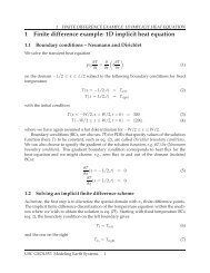
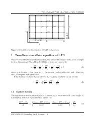
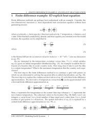
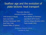
Figure1: Discretizationforthestreamfunctionapproach. Theboundaryconditionsaresetthrough
fictiousboundarypoints.
1 <strong>Stokes</strong> <strong>equations</strong> <strong>with</strong> <strong>FD</strong> on a staggered grid using the
stream-functionapproach.
1.1 Introduction
As was discussed in sec. ??, the basis of basically all mantle convection and lithospheric
dynamicscodes are the <strong>Stokes</strong> <strong>equations</strong> for slowly movingviscous fluids.
There are several ways to solve those <strong>equations</strong>, and the goal of this exercise is to
use a streamfunction, finite difference approach. Stream function means that there is a
potential field which we solve for, and then obtain velocities from the derivatives of this
field. The advantage of this approach is that the continuity equation for incompressible
flow can be satisfied implicitly, rather than having to use a panelty parameter as for the
primitive variable approach of sec. ??. (It is, however, possible to formulate the stream
function method for compressible convection approximations, e.g. ?). For a comparison
ofdifferent finite difference approaches, see ?, for example.
Themainchallengesofthisprojectare,1),havingfairlyhigh-orderandmixedderivatives
(up to4 th order) and,2), setting of boundaryconditions.
1.2 Governing<strong>equations</strong>
It is assumed that the rheology is incompressible and that the rheology is Newtonian
viscous. In thiscase, the governing <strong>equations</strong>are (see sec. ??):
USCGEOL557: ModelingEarth Systems 1

1 STOKES EQUATIONSWITH<strong>FD</strong> ON ASTAGGEREDGRIDUSINGTHE
STREAM-FUNCTIONAPPROACH.
∂v x
∂x + ∂v z
= 0
∂z
(1)
∂σ xx
∂x + ∂σ xz
= 0
∂z
(2)
∂σ xz
∂x + ∂σ zz
− ρg = 0
∂z
(3)
σ xx = −p +2µ ∂v x
∂x
σ zz = −p +2µ ∂v z
( ∂z
∂vx
σ xz = µ
∂z + ∂v )
z
∂x
Bysubstituting eqs.(4)-(6) into eqs.(1)-(3), weobtain (compare sec. ??)
− ∂p
∂x +2 ∂ (
∂x
− ∂p
∂z +2 ∂ ∂z
µ ∂v x
∂x
(
µ ∂v z
∂z
∂v x
∂x + ∂v z
)
∂z
+ ∂ ( ( ∂vx
µ
∂z ∂z + ∂v ))
z
∂x
)
+ ∂ ( ( ∂vx
µ
∂x ∂z + ∂v ))
z
∂x
(4)
(5)
(6)
= 0 (7)
= 0 (8)
= ρg (9)
We can eliminate pressure from eqs. (8) and (9) by taking the derivative of eq. (8) versus
z andsubtracting eq. (9)derivedversus x. Thisresults in:
(
2 ∂2
µ ∂v (
x
)−2 ∂2
µ ∂v )
z
+
∂x∂z ∂x ∂x∂z ∂z
∂ 2 ( ( ∂vx
∂z 2 µ
∂z + ∂v ( (
z
))− ∂2 ∂vx
∂x ∂x 2 µ
∂z + ∂v ))
z
= − ∂ ρg. (10)
∂x
∂x
Wecan alsouse the incompressibility constraint (7)to simplify things alittle bitmore:
(
−4 ∂2
µ ∂v )
z
+
∂x∂z ∂z
∂ 2 ( ( ∂vx
∂z 2 µ
∂z + ∂v ( (
z
))− ∂2 ∂vx
∂x ∂x 2 µ
∂z + ∂v ))
z
= − ∂ ρg (11)
∂x
∂x
Now we introduce a variable Ψ (the stream function) which is defined by its relationship
to the velocities as
v x = ∂Ψ
∂z
v z = − ∂Ψ
∂x
USCGEOL557: ModelingEarth Systems 2
(12)
(13)

1 STOKES EQUATIONSWITH<strong>FD</strong> ON ASTAGGEREDGRIDUSINGTHE
STREAM-FUNCTIONAPPROACH.
Note that Ψ satisfies incompressibility byplugging eqs. (12)and(13)into eq.(1).
Byusing Ψ, we can write eq. (11)as:
∂ 2 ( ( ∂ 2 )) (
Ψ
∂z 2 µ
∂z 2 − ∂2 Ψ
∂x 2 − ∂2
∂x 2 µ
4 ∂2
( )
µ ∂2 Ψ
∂x∂z
∂x∂z
( ∂ 2 ))
Ψ
∂z 2 − ∂2 Ψ
∂x 2
+
= − ∂ ρg. (14)
∂x
Note that this equation now has 4 th order derivatives for Ψ (easier to see for constant µ,
where we can pull the viscosity out of the derivatives.) The challenge is to solve eq. (14)
for Ψ given then density gradients.
1.3 Exercise
1. Discretize eq.(14)on a grid asshown on Figure 1.
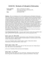
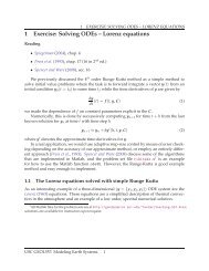
2. A MATLAB subroutine is shown on Figure 2. The subroutine sets up the grid and
the node numbering. Finish the code by programming the discretized eq. (14). To
start simple, assume thatviscosity isconstant.
3. Addfree-slip boundary conditions on all sides(which means v z = 0, σ xz = 0on the
lowerandupperboundariesand σ xz = 0,v x = 0onthesideboundaries;you’llhave
to write these <strong>equations</strong> in termsof Ψ andemploy fictious boundary points).
4. Assume a model domain x = [0;1], z = [0;1], and assume that the density below
z = 0.1cos(2πx) +0.5 is1, whereas the density above it is 2. Compute the velocity,
andplot the velocity vectors.
5. Writethecodeforthecaseofvariableviscosity(whichisrelevantfortheEarthsince
rock properties are a strong function of temperature).
USCGEOL557: ModelingEarth Systems 3

1 STOKES EQUATIONSWITH<strong>FD</strong> ON ASTAGGEREDGRIDUSINGTHE
STREAM-FUNCTIONAPPROACH.
% Solve the 2D <strong>Stokes</strong> <strong>equations</strong> on a staggered grid, using the Vx,Vz,P
% formulation.
clear
% Material properties phase #1 phase #2
mu_vec = [1 1 ];
rho_vec = [1 2 ];
% Input parameters
Nx = 6;
Nz = 6;
W = 1;H = 1;g = 1;
% Setup the interface
x_int = 0:.01:W;
z_int = cos(x_int*2*pi/W)*1e-2 - 0.5;
% Setup the grids----------------------------------------------------------
dz = H/(Nz-1);dx = W/(Nx-1);
[X2d,Z2d] = meshgrid(0:dx:W,-H:dz:0);
%--------------------------------------------------------------------------
% Compute material properties from interface-------------------------------
% Properties are computed in the center of a control volume
Rho = ones(Nz,Nx)*rho_vec(2);
Mu = ones(Nz,Nx)*mu_vec(2);
z_int_intp = interp1(x_int,z_int,X2d(1,:));
for ix = 1:length(z_int_intp)
ind = find(Z2d(:,1)

BIBLIOGRAPHY
Bibliography
USCGEOL557: ModelingEarth Systems 5