FINITE ELEMENT METHODS - Solid Mechanics Home Page - Caltech

FINITE ELEMENT METHODS: 1970’s AND BEYOND
L.P. Franca (Ed.)
c○ CIMNE, Barcelona, Spain 2003
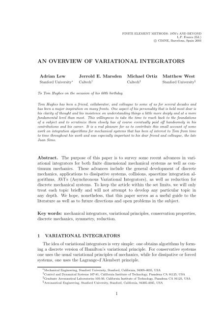
AN OVERVIEW OF VARIATIONAL INTEGRATORS
Adrian Lew Jerrold E. Marsden Michael Ortiz Matthew West
Stanford University ∗ Caltech † Caltech ‡ Stanford University §
To Tom Hughes on the occasion of his 60th birthday
Tom Hughes has been a friend, collaborator, and colleague to some of us for several decades and
has been a major inspiration on many fronts. One aspect of his personality that is held most dear is
his clarity of thought and his insistence on understanding things a little more deeply and at a more
fundamental level than most. This willingness to take the time to reach back to the foundations
of a subject and to scrutinize them closely has of course eventually paid off handsomely in his
contributions and his career. It is a real pleasure for us to contribute this small account of some
work on integration algorithms for mechanical systems that has been of interest to Tom from time
to time throughout his work and was especially important to his dear friend and colleague, the late
Juan Simo.
Abstract. The purpose of this paper is to survey some recent advances in variational
integrators for both finite dimensional mechanical systems as well as continuum
mechanics. These advances include the general development of discrete
mechanics, applications to dissipative systems, collisions, spacetime integration algorithms,
AVI’s (Asynchronous Variational Integrators), as well as reduction for
discrete mechanical systems. To keep the article within the set limits, we will only
treat each topic briefly and will not attempt to develop any particular topic in
any depth. We hope, nonetheless, that this paper serves as a useful guide to the
literature as well as to future directions and open problems in the subject.
Key words: mechanical integrators, variational principles, conservation properties,
discrete mechanics, symmetry, reduction.
1 VARIATIONAL INTEGRATORS
The idea of variational integrators is very simple: one obtains algorithms by forming
a discrete version of Hamilton’s variational principle. For conservative systems
one uses the usual variational principles of mechanics, while for dissipative or forced
systems, one uses the Lagrange-d’Alembert principle.
∗ Mechanical Engineering, Stanford University, Stanford, California, 94305-4035, USA
† Control and Dynamical Systems 107-81, California Institute of Technology, Pasadena CA 91125, USA
‡ Graduate Aeronautical Laboratories 105-50, California Institute of Technology, Pasadena CA 91125, USA
§ Aeronautical Engineering, Stanford University, Stanford, California, 94305-4035, USA
1

Finite Element Methods: 1970’s and beyond
Hamilton’s Configuration Space Principle. Let us begin with the case of
finite dimensional systems first. We now recall from basic mechanics (see, for example,
Marsden and Ratiu [1999]) the configuration space form of Hamilton’s principle.
Let a mechanical system have an n-dimensional configuration manifold Q (with a
choice of coordinates denoted by q i , i = 1, . . ., n) and be described by a Lagrangian
L : TQ → R, denoted in coordinates by L(q i , ˙q i ). Then the principle states that the
action integral is stationary for curves in Q with fixed endpoints; this principle is
commonly denoted (see Figure 1.1).
δ
∫ b
a
L(q, ˙q) dt = 0.
q(t)
varied curve
Q
q(a)
q(t)
q(b)
Figure 1.1: The configuration space form of Hamilton’s principle
With appropriate regularity assumptions, Hamilton’s principle, as is well-known,
is equivalent to the Euler–Lagrange equations
d ∂L
dt ∂ ˙q − ∂L
i ∂q = 0. i
Discrete Configuration Space Mechanics. In discrete mechanics from the Lagrangian
point of view, which has its roots in discrete optimal control from the 1960’s
(see Marsden and West [2001] and Lew, Marsden, Ortiz, and West [2004] for accounts
of the history and related literature), one first forms a discrete Lagrangian,
a function L d of two points q 1 , q 2 ∈ Q and a time step h by approximating the the
action integral along an exact trajectory with a quadrature rule:
L d (q 0 , q 1 , h) ≈
∫ h
0
L ( q(t), ˙q(t) ) dt
where q(t) is an exact solution of the Euler–Lagrange equations for L joining q 0 to
q 1 over the time step interval 0 ≤ t ≤ h. Recall that Jacobi’s theorem from 1840
states that using the exact value and not an approximation would lead to a solution
to the Hamilton–Jacobi equation. This is depicted in Figure 1.2 (a) and points out
a key link with Hamilton–Jacobi theory.
Holding h fixed at the moment, we regard L d as a mapping L d : Q × Q → R.
This way of thinking of the discrete Lagrangian as a function of two nearby points
(which take the place of a discrete position and velocity) goes back to the origins of
Hamilton–Jacobi theory itself, but appears explicitly in the discrete optimal control
literature in the 1960s, and was exploited effectively by, for example, Suris [1990];

A. Lew, J. E.Marsden, M. Ortiz, M. West/VARIATIONAL INTEGRATORS
Q
q i
varied point
q(t), an exact solution
q 1
q 0
t = h
t = 0
Q
q 0
δq i
q N
(a)
(b)
Figure 1.2: The discrete form of the configuration form of Hamilton’s principle
Moser and Veselov [1991]; Wendlandt and Marsden [1997]. It is a point of view that
is crucial for the development of the theory.
Given a discrete Lagrangian L d , the discrete theory proceeds in its own right
as follows. Given a sequence q 1 , . . ., q N of points in Q, form the discrete action
sum:
S d =
N−1
∑
k=0
L d (q k , q k+1 , h k ).
Then the discrete Hamilton configuration space principle requires us to seek a critical
point of S d with fixed end points, q 0 and q N . Taking the special case of three
points q i−1 , q i , q i+1 , so the discrete action sum is L d (q i−1 , q i , h i−1 ) + L d (q i , q i+1 , h i )
and varying with respect to the middle point q i gives the DEL (discrete Euler–
Lagrange) equations:
D 2 L d (q i−1 , q i , h i−1 ) + D 1 L d (q i , q i+1 , h i ) = 0. (1.1)
One arrives at exactly the same result using the full discrete variational principle.
The equations 1.1 defines, perhaps implicitly, the DEL algorithm: (q i−1 , q i ) ↦→
(q i , q i+1 ).
Example. Let M be a positive definite symmetric n × n matrix and V : R n → R
be a given potential. Choose a discrete Lagrangian on R n × R n of the form
[( ) T ( )
q1 − q 0 q1 − q 0
L d (q 0 , q 1 , h) = h M
h h
]
− V (q 0 ) , (1.2)
which arises in an obvious way from its continuous counterpart by using simply a
form of “rectangle rule” on the action integral. For this discrete Lagrangian, the
DEL equations are readily worked out to be
( )
qk+1 − 2q k + q k−1
M
= −∇V (q
h 2 k ),
a discretization of Newton’s equations, using a simple finite difference rule for the
derivative.
Somewhat related to this example, it is shown in Kane, Marsden, Ortiz, and
West [2000] that the widely used Newmark scheme (see Newmark [1959]) is also
variational in this sense as are many other standard integrators, including the midpoint
rule, symplectic partitioned Runge–Kutta schemes, etc.; we refer to Marsden

Finite Element Methods: 1970’s and beyond
and West [2001] (see also Suris [1990]) for details. Of course, Tom’s book (Hughes
[1987]) is one of the standard sources for the Newmark algorithm). Some of us have
come to the belief that the variational nature of the Newmark scheme is one of the
reasons for its excellent performance.
Hamilton’s Phase Space Principle. We briefly mention the Hamiltonian point
of view; now we are given a Hamiltonian function H : T ∗ Q → R, where T ∗ Q is the
cotangent bundle of Q, on which a coordinate choice is denoted (q 1 , . . .q n , p 1 , . . .,p n ).
In this context one normally uses the phase space principle of Hamilton, which states
that for curves (q(t), p(t)) in T ∗ Q, with fixed endpoints, that the phase space action
integral be stationary:
δ
∫ b
a
(
pi dq i − H(q i , p i ) ) dt = 0. (1.3)
Of course, p i dq i is the coordinate form of the canonical one-form Θ which has the
property that dΘ = −Ω = ∑ dq i ∧ dp i , the standard symplectic form. Again,
under appropriate regularity conditions, this phase space principle is equivalent to
Hamilton’s equations:
dq i
dt = ∂H
∂p i
;
dp i
dt = −∂H ∂q i . (1.4)
Discrete Hamilton’s Phase Space Principle. There are some different choices
of the form of the discrete Hamiltonian, corresponding to different forms of generating
functions, but perhaps the simplest and most intrinsic one is a function
H d : T ∗ Q × R → R, where H d (q, p, h). As in the Lagrangian case, H d is an approximation
of the action integral:
H d (q, p, h) ≈
∫ h
0
(
pi (t)dq i (t) − H(q i (t), p i (t)) ) dt, (1.5)
where (q(t), p(t)) ∈ T ∗ Q is the unique solution of Hamilton’s equations with (q(0),
p(0)) = (q, p). We do not discuss the Hamiltonian point of view here, but rather refer
to the work of Lall and West [2004] for more information. Many algorithms, such
as the midpoint rule and symplectic Runge–Kutta schemes, appear more naturally
from the Hamiltonian point of view, as discussed in Marsden and West [2001].
In addition, some problems, such as the dynamics of point vortices discussed in
Rowley and Marsden [2002] and below, involved degenerate Lagrangians, but have
a nice Hamiltonian formulation. In this case, it seems that there is a definite numerical
advantage to using a Hamiltonian formulation directly without going via the
Lagrangian formalism. For instance, the discrete Euler–Lagrange equations corresponding
to a degenerate continuous Lagrangian may attempt to treat the equations
as second order equations, whereas the continuous equations are, in reality, first order.
The Lagrangian approach can, for these reasons, lead to potential instabilities
due to multi-step algorithms (such as the leapfrog scheme) and so one would have
to be very careful in the choice of parameters, as is done in Rowley and Marsden
[2002]. It seems that a direct Hamiltonian approach avoids these issues and so is
one reason for their usefulness.

A. Lew, J. E.Marsden, M. Ortiz, M. West/VARIATIONAL INTEGRATORS
2 PROPERTIES OF VARIATIONAL INTEGRATORS
We shall demonstrate through some specific examples that variational integrators
work very well for both conservative and dissipative or forced mechanical systems
in a variety of senses. Some specific properties of variational integrators that make
them attractive are given in the following paragraphs.
Structure Preservation. No matter what the choice of the discrete Lagrangian,
variational integrators are, for the non-dissipative and non-forced (that is the conservative)
case, symplectic and momentum conserving. Momentum preserving means
that when the discrete system has a symmetry, then there is a discrete Noether
theorem that gives a quantity that is exactly conserved at the discrete level. Figure
2.1(a) illustrates the sort of qualitative difference that structure preserving gives in
solar system dynamics and in (b) we illustrate that symplectic in the case of two
dimensional systems means area preserving, even with large distortions.
(a)
(b)
Figure 2.1: (a) Variational integrators give good qualitative behavior for comparable computational
effort. (b) Variational integrators preserve the symplectic form in phase space (area in two
dimensions). These figures are due to Hairer, Lubich, and Wanner [2001], to which we refer for
further information.
Marsden and West [2001] give a detailed discussion of discrete mechanics in the
finite dimensional case, the associated numerical analysis and for a variational proof
of the symplectic property and the discrete conservation laws. We also note that this
theory shows the sense in which, for example, the Newmark scheme is symplectic;
some people have searched in vain by hand to try to discover a conserved symplectic
form for the Newmark algorithm—but it is hidden from view and it is the variational
technique that evokes it!
One can check the conservation properties by direct computation (see Wendlandt
and Marsden [1997]) or what is more satisfying, one can derive them directly from the
variational nature of the algorithm. In fact, the symplectic nature of the algorithm
results from the boundary terms in the variational principle when the endpoints are
allowed to vary. This argument is due to Marsden, Patrick, and Shkoller [1998].
Another remark is in order concerning both the symplectic nature as well as the
Noether conserved quantities. In the continuous theory, the conserved symplectic
structure is given, in the Lagrangian picture, by the differential two-form Ω = dq i ∧
dp i , where a sum on i is understood and p i = ∂L/∂ ˙q i . One has to be careful about

Finite Element Methods: 1970’s and beyond
what the discrete counterpart of Ω is. Trial and error, which has been often used, is
of course very inefficient. Fortunately, the theory produces automatically the correct
conserved form, a two-form on Q×Q, just from the variational nature of the problem
by mimicking the continuous proof. Similar remarks apply to the case of the Noether
conserved quantities.
It should be also noted that there are deep links between the variational method
for discrete mechanics and integrable systems. This area of research was started by
Moser and Veselov [1991] and was continued by many others, notably by Bobenko
and Suris; we refer the reader to the book Suris [2003] for further information.
The main and very interesting example studied by Moser and Veselov [1991] was
to find an integrable discretization of the n-dimensional rigid body, an integrable
system; see also Bloch, Crouch, Marsden, and Ratiu [2002] for further insight into
the discretization process in this case.
A bit more history that touches Tom personally is perhaps in order at this point.
We need to recall, first of all, that Tom has had a long interest in energy preserving
schemes, for example, in his work with Caughey (see Chorin, Hughes, Marsden,
and Mccracken [1978] and references therein). We also need to recall that a result
of Ge and Marsden [1988] states that typically integrators with a fixed time step
cannot simultaneously preserve energy, the symplectic structure and conserved quantities.
“Typically” means for instance that integrable systems can be an exception
to this rule. This result led to a dichotomy in the literature between symplecticmomentum
and energy-momentum integrators; the late Juan Simo was a champion
of the energy-momentum approach, as discussed in, for instance Simo, Tarnow, and
Wong [1992], Gonzalez and Simo [1996], and Gonzalez [1996]. On the other hand,
one can “have it all” if one uses adaptive schemes, as in Kane, Marsden, and Ortiz
[1999]. However, for reasons of numerical efficiency and because of the remarkable
energy behavior of symplectic schemes (discussed below), it seems that symplecticmomentum
methods are the methods of choice at the moment, although adaptation
is a key issue discussed further in the context of AVI methods below.
Integrator Design. A nice feature of the variational approach to symplectic integrators
is that it leads to a systematic construction of higher-order integrators, which
is much easier than finding approximate solutions to the Hamilton–Jacobi equation,
which is the original methodology (discussed in, for example, De Vogelaére [1956],
Ruth [1983] and Channell and Scovel [1990]). For instance, by taking appropriate
Gauss–Lobatto quadrature approximations of the action function, one arrives in a
natural way at the SPARK (symplectic partitioned adaptive Runge–Kutta) methods
of Jay [1996] (see also Belytschko [1981] and Grubmüller et. al. [1991]); this
is shown in Marsden and West [2001]. It is also notable that these integrators are
flexible, they include explicit or implicit algorithms; thus, in the design, there is no
bias towards either type of integrator. In addition, the variational methodology has
led to the important notion of multisymplectic integrators, discussed below.
Accuracy and Energy Behavior. In Marsden and West [2001] it is shown that
the order of approximation of the action integral is reflected in the corresponding
order of approximation for the algorithm. For instance, this is the general reason
that the Newmark algorithm is second order accurate and why the SPARK schemes

A. Lew, J. E.Marsden, M. Ortiz, M. West/VARIATIONAL INTEGRATORS
can be designed to be higher order accurate. A corresponding statement for the
PDE case is given in Lew, Marsden, Ortiz, and West [2004]. The notion of Γ-
convergence is also emerging as a very important notion for variational integrators
and this aspect is investigated in Müller and M. Ortiz [2004].
Variational integrators have remarkably good energy behavior in both the conservative
and dissipative cases (for the latter, recall that one discretizes the Lagrange-d’Alembert
principle); consider, for example, the system described in Figure 2.2,
namely a particle moving in the plane.
0.35
Midpoint Newmark
0.3
0.3
0.25
0.25
Energy
0.2
0.15
Benchmark
Variational Explicit Newmark
non-variational Runge-Kutta
Energy
0.2
0.15
Variational
0.1
0.1
Runge-Kutta
0.05
0.05
Benchmark
0
0 100 200 300 400 500 600 700 800 900 1000
Time
(a) Conservative mechanics
0
0 200 400 600 800 1000 1200 1400 1600
Time
(b) Dissipative mechanics
Figure 2.2: Showing the excellent energy behavior for both conservative and dissipative systems: a
particle in R 2 with a radially symmetric polynomial potential (left); with small dissipation of the
standard sort (proportional to the velocity) (right).
This figure illustrates the fact that variational integrators have long time energy
stability (as long as the time step is reasonably small). This is a key property,
but it is also a deep one from the theoretical point of view and is observed to
hold numerically in many cases when the theory cannot strictly be verified; the
key technique is known as backward error analysis and it seeks to show that the
algorithm is, up to exponentially small errors, the exact time integration of a nearby
Hamiltonian system, an idea going back to Neishtadt [1984]. See, for instance, Hairer
and Lubich [2000] for an excellent analysis.
But there are many unanswered questions. For instance, apart from the numerical
evidence, a corresponding theory for the dissipative case is not known at the present
time. Some progress is being made on the PDE case, but the theory still has a long
way to go; see, for instance Oliver, West, and Wulff [2004]. For this example, in the
absence of dissipation the variational algorithms are exactly symplectic and angular
momentum preserving—if one were to plot a measure of these quantities, one would
just see a horizontal line, confirming the theory that this is indeed always the case.
Computing Statistical Quantities. Variational integrators have some other interesting
properties having to do with the accurate computation of statistical quantities.
One should not think that individual trajectories are necessarily computed
accurately in a chaotic regime, but it does seem that important statistical quantities
are computed correctly. In other words, these integrators somehow “get the physics
right”.
We give two examples of such behavior. The first of these (see Figure 2.3),
taken from Rowley and Marsden [2002], is the computation of chaotic invariant

Finite Element Methods: 1970’s and beyond
sets in the four point vortex dynamics in the plane. As mentioned previously, the
Lagrangian for this problem is degenerate and so one has to be careful with both
the formulation and the numerics. As mentioned previously, if one uses Hamilton’s
phase space principle directly on this problem, things are somewhat improved. The
figure shows a Poincaré section for this problem in a chaotic regime. It clearly shows
that variational integrators produce the structure of the chaotic invariant set more
accurately than (non symplectic) Runge–Kutta algorithms, even more accurate ones.
Figure 2.3: Variational integrators capture well the structure of chaotic sets; RK4 is a fourth order
Runge–Kutta algorithm, while VI2 is a second order accurate variational integrator. The time step
is h = ∆t. Both schemes produce clear Poincaré sections for h = 0.2, but for h = 0.5, scheme RK4
produces a blurred section, while the section from scheme VI2 remains crisp even for h = 1.0. For
h = 1.0, scheme RK4 deviates completely, and transitions into a spurious quasiperiodic state.
Another interesting statistical quantity is the computation of the “temperature”
(strictly speaking, the “heat content”, or the time average of the kinetic energy)
of a system of interacting particles, taken from Lew, Marsden, Ortiz, and West
[2004] and shown in Figure 2.4. Of course the “temperature” is not associated with
any conserved quantity and nevertheless variational integrators give a well defined
temperature over what appears to be an indefinite integration time, while standard
integrators eventually deviate and again give spurious results.
Discrete Reduction Theory. Reduction theory is an indispensable tool in the
study of many aspects of mechanical systems with symmetry, such as stability of relative
equilibria by the energy–momentum method. See Marsden and Weinstein [2001]
for a review of the many facets of this theory and for references. It is natural to seek
discrete analogs of this theory. Motivated by the work of Moser and Veselov [1991],
the first version of discrete reduction that was developed was the discrete analog of
Euler–Poincaré reduction, which reduces second-order Euler–Lagrange equations on
a Lie group G to first order dynamics on its Lie algebra g. Examples of this sort of
reduction are the Euler equations for a rigid body and the Euler equations for an
ideal fluid. The discrete version of this gives the DEL or Discrete Euler–Lagrange
equations. These equations were investigated by Marsden, Pekarsky, and Shkoller
[1999, 2000] and Bobenko and Suris [1999,?] (who also made some interesting links
with integrable structures and semi-direct products).

A. Lew, J. E.Marsden, M. Ortiz, M. West/VARIATIONAL INTEGRATORS
Average kinetic energy
0.045
0.04
0.035
0.03
0.025
∆ t = 0.5
∆ t = 0.2
∆ t = 0.1
∆ t = 0.05
RK4
VI1
lskdjf sldkfj
∆ t = 0.05
∆ t = 0.1
∆ t = 0.2
∆ t = 0.5
0.02
10 0 10 1 10 2 10 3 10 4 10 5
Time
Figure 2.4: Variational integrators capture statistically significant quantities, such as the heat
content of a chaotic system. The average kinetic energy as a function of the integration run T for
a nonlinear spring–mass lattice system in the plane, using a first order variational integrator (VI1)
and a fourth order Runge–Kutta method (RK4) and a range of timesteps ∆t. Observe that the
Runge–Kutta method suffers substantial numerical dissipation, unlike the variational method.
Another step forward was made by Jalnapurkar, Leok, Marsden, and West [2004]
who developed discrete reduction for the case of Routh reduction; that is, one fixes
the value of the momentum conjugate to cyclic variables and drops the dynamics to
the quotient space. This was applied to the case of satellite dynamics for an oblate
Earth (the J 2 problem) and to the double spherical pendulum. Already this case is
interesting because these examples exhibit geometric phases and the reduction allows
one to “separate out” the phase shift and thereby avoid any spurious numerical
phases.
It is clear that discrete reduction should continue to develop. For instance, in
addition to the nonabelian case of Routh reduction (due to Marsden, Ratiu, and
Scheurle [2000]), one should develop the DLP (Discrete Lagrange–Poincaré) and
DHP (Discrete Hamilton–Poincaré) equations. The continuous LP and HP equations
are discussed in Cendra, Marsden, and Ratiu [2001, 2003]. Of course, counterparts
on the Hamiltonian side should also be developed.
3 MULTISYMPLECTIC AND AVI INTEGRATORS
One of the beautiful and simple things about the variational approach is that it
suggests an extension to the PDE case. Namely one should discretize, in space-time,
the variational principle for a given field theory, such as elasticity. This variational
formulation of elasticity is well known and is described in many books, such as Marsden
and Hughes [1983]. The idea is to extend the discrete formulation of Hamilton’s
principle discussed at the beginning of this article to an analogous discretization of
a field theory. One replaces the discrete time points with a mesh in spacetime and
replaces the points in Q with clusters of points (so that one can represent the needed
derivatives of the fields) of field values.
Another historical note involving Tom is relevant here. Tom was always interested
in and pushed the idea that one should ultimately do things in spacetime and not
just in space with fixed time steps. He explored this idea in various papers, such as
Masud and Hughes [1997] and Hughes and Stewart [1996] and even going back to
Hughes and Hulbert [1988]. The AVI method is developed in the same spirit.

Finite Element Methods: 1970’s and beyond
The Setting of AVI Methods. The basic set up and feasibility of this idea in
a variational multisymplectic context was first demonstrated in Marsden, Patrick,
and Shkoller [1998] who used the sine-Gordon equation to illustrate the method numerically.
The paper also showed that there were discrete field theoretic analogs of
all the structures one has in finite dimensional mechanics with some modifications;
the symplectic structure gets replaced by a multisymplectic structure (using differential
forms of higher degree) and analogs of discrete Noether quantities. As in the
case of finite dimensional mechanics, all of these properties follow from the fact that
one has a discrete variational principle. The appropriate multisymplectic formalism
setting that set the stage for discrete elasticity was given in Marsden, Pekarsky,
Shkoller, and West [2001]. Motivated by this work, Lew, Marsden, Ortiz, and West
[2003] developed the theory of AVIs (Asynchronous Variational Integrators) along
with an implementation for the case of elastodynamics. These integrators are based
on the introduction of spacetime discretizations allowing different time steps for
different elements in a finite element mesh along with the derivation of time integration
algorithms in the context of discrete mechanics, i.e., the algorithm is given by
a spacetime version of the Discrete Euler–Lagrange (DEL) equations of a discrete
version of Hamilton’s principle.
The spacetime bundle picture provides an elegant generalization of Lagrangian
mechanics, including temporal, material and spatial variations and symmetries as
special cases. This unites energy, configurational forces and the Euler–Lagrange
equations within a single picture. The geometric formulation of the continuous theory
is used to guide the development of discrete analogues of the geometric structure,
such as discrete conservation laws and discrete (multi)symplectic forms. This is one
of the most appealing aspects of this methodology.
To reiterate the main point, the AVI method provides a general framework for
asynchronous time integration algorithms, allowing each element to have a different
time step, similar in spirit to subcycling (see, for example, Neal and Belytschko
[1989]), but with no constraints on the ratio of time step between adjacent elements.
A local discrete energy balance equation is obtained in a natural way in the AVI
formalism. This equation is expected to be satisfied by adjusting the elemental time
steps. However, as was mentioned before, it is sometimes computationally expensive
to do this exactly and from simulations (such as the one given below), it seems to
be unnecessary. That is, the phenomenon of near energy conservation indefinitely
in time appears to hold, just as in the finite dimensional case. As was mentioned
already, the full theory of a backward error analysis in the PDE context is in its
infancy (see Oliver, West, and Wulff [2004]).
Elastodynamics Simulation. The formulation and implementation of a sample
algorithm (explicit Newmark for the time steps) is given in this framework. An
important issue is how it is decided which elements to update next consistent with
hyperbolicity (causality) and the CFL condition. In fact, this is a nontrivial issue
and it is accomplished using the notion of a priority queue borrowed from computer
science. Figure 3.1 shows one snapshot of the dynamics of an elastic L-beam (the
beam is undergoing oscillatory deformations). The smaller elements near the edges
are updated much more frequently than the larger elements.

A. Lew, J. E.Marsden, M. Ortiz, M. West/VARIATIONAL INTEGRATORS
Total Energy [MJ]
654
653
652
651
650
649
648
0 10 20 30 40 50 60 70 80 90 100
t[ms]
Figure 3.1: AVI methods are used to simulate the dynamics of an elastic L-beam. The energy of
the L-beam is nearly constant after a long integration run with millions of updates of the smallest
elements.
The figure also shows the very favorable energy behavior for the L-beam obtained
with AVI techniques; the figure shows the total energy, but it is important to note
that also the local energy balance is excellent—that is, there is no spurious energy
exchange between elements as can be obtained with other elements. In fact, by
computing the discrete Euler–Lagrange equation for the discrete action sum corresponding
to each elemental time step, a local energy equation is obtained. This
equation is not generally enforced, and the histogram in Figure 3.2 shows the distribution
of maximum relative error in satisfying the local energy equation on each
element for a two-dimentsional nonlinear elastodynamics simulation. The relative
error is defined as the absolute value of the quotient between the residual of the the
local energy equation and the instantaneous total energy in the element. More than
50% of the elements have a maximum relative error smaller than 0.1%, while 97.5%
of the elements have a maximum relative error smaller that 1%. This test shows
that the local energy behavior of AVI is excellent, even though it is not exactly
enforced.
Number of elements
60
50
40
30
20
10
0
0.0001 0.001 0.01 0.1 1
Maximum Relative Error
Figure 3.2: Local energy conservation for a two-dimensional nonlinear elastodynamics simulation.
These issues of small elements (sliver elements) are even more pronounced in other
examples such as rotating elastic helicopter blades (without the hydrodynamics)
which have also been simulated in some detail. The Helicopter blade is one of the
examples that was considered by the late Juan Simo who showed that standard (and

Finite Element Methods: 1970’s and beyond
even highly touted) algorithms can lead to troubles of various sorts. For example,
if the modeling is not done carefully, then it can lead to spurious softening and
also, even though the algorithm may be energy respecting, it can be very bad as far
as angular momentum conserving is concerned. The present AVI techniques suffer
from none of these difficulties. This problem is discussed in detail in Lew [2003] and
West [2004].
Networks and Optimization. One of the main points of the AVI methodology
is that it is spatially distributed in a natural way and hence it suggests that one
should seek a unification of its ideas with those used in network optimization, where
in the primal–dual methodology, there is an iteration between local updates for
optimization and then message passing. For example, this is one of the main things
going on in TCP/IP protocols, which in reality are AVI methods! This aspect of
the theory is currently under development in Lall and West [2004] and represents a
very exciting direction of current research.
4 COLLISIONS
Another major success of variational methods is in collision problems, both finite
dimensional (particles, rigid bodies, etc) and elastic (elastic solids as well as). We
refer to Fetecau, Marsden, Ortiz, and West [2003] for the complex history of the subject.
In fact, most of the prior approaches to the problem are based on smoothing,
on penalty methods or on weak formulations. All of these approaches suffer from
difficulties of one sort or another. Our approach, in contrast, is based on a variational
methodology that goes back to Young [1969]. For the algorithms, we combine
this variational approach with the discrete discrete Lagrangian principle together
with the introduction of a collision point and a collision time, which are solved for
variationally. This variational methodology allows one to retain the symplectic nature
as well as the remarkable near energy preserving properties (or correct decay
in the case of dissipative problems–inelastic collisions) even in the non-smooth case.
A key first step is to introduce, for the time continuous case, a space of configuration
trajectories including curve parametrizations as variables, so that the traditional
approach to the calculus of variations can be applied. This extended setting enables
one to give a rigorous interpretations to the sense in which the flow map of a mechanical
system subjected to dissipationless impact dynamics is symplectic in a way
that is consistent with Weierstrass–Erdmann type conditions for impact, in terms of
energy and momentum conservation at the contact point. The discrete variational
formalism leads to symplectic-momentum preserving integrators consistent with the
jump conditions and the continuous theory. The basic idea is shown in Figure 4.1
in which the points q i are varied in the discrete action sum, just as in the general
DEL algorithm, but in addition, the point ˜q is inserted on the boundary and the
variable time of collision through the parameter α are introduced. One has just the
right number of equations to solve for ˜q and α from the variational principle.
An important issue is how nonsmooth analysis techniques—based on the Clarke
calculus (see Clarke [1983] and Kane, Repetto, Ortiz, and Marsden. [1999])—can
be incorporated into the variational procedure for elastic collisions, such that the
integrator can cope with nonsmooth contact geometries (corner to corner collisions,

A. Lew, J. E.Marsden, M. Ortiz, M. West/VARIATIONAL INTEGRATORS
q i + 1
q i – 2
h
h
q i
q i – 1
αh
(1 − α)h
q ~
M
boundary of the admissible
set (the collision set)
Figure 4.1: The basic geometry of the collision algorithm.
for instance). This is a case which most existing algorithms cannot handle very
well (the standard penalty methods simply fail since no proper gap function can be
defined for such geometries). We should also note that friction can be incorporated
into these methods using, following our general methodology, the Lagrange-d’Alembert
principle or similar optimization methods for handling dissipation. This is
given in Pandolfi, Kane, Marsden, and Ortiz [2002].
Closely related methods have been applied to the difficult case of shell collisions
in Cirak and West [2004], which are handled using a combination of ideas from AVI,
subdivision, velocity decompositions and collision methods similar to those described
above, along with some important spatially distributed parallelization techniques for
computational efficiency. We show an example of such a collision between two thin
shells in Figure 4.2. Similar methods have been applied to the case of colliding
beams and to airbag inflation. In such problems, the numerous near coincidental
self collisions presented a major hurdle.
Figure 4.2: AVI methodology: collision between an elastic sphere and a plate (Cirak and West
[2004].
5 SHOCK CAPTURING FOR A CONTAINED EXPLOSION
Lew [2003] has applied the AVI methodology to the case of shocks in high explosives.
The detonation is initiated by impacting one of the planar surfaces of the
set canister-explosive. The time steps of the elements are dynamically modified to
track the front of the detonation wave and capture the chemical reaction time scales.

Finite Element Methods: 1970’s and beyond
Figure 5.1 (parts I and II) shows the evolution of the number of elemental updates
during a preset time interval (lower half of each snapshot) and the pressure contours
(upper half of each snapshot), both in the explosive and in the surrounding solid.
The plots of the number of elemental updates only show values on a plane of the
cylinder that contains its axis, and can be roughly described as composed of three
strips. The central strip, which lies in the explosive region, has fewer elemental
updates than the two thin lateral strips, which lie in the solid canister region. This
corresponds to having neighboring regions with different sound speeds and therefore
different time steps given by the Courant condition.
Figure 5.1 (part I): Evolution of a detonation wave within a nonlinear solid canister.
6 ADDITIONAL REMARKS AND CONCLUSIONS
It is perhaps worth pointing out that AVI methods are (perhaps without some
of the users realizing it) are already being used in molecular dynamics; see, for
example, Tuckerman, Berne, and Martyna [1992], Grubmüller et. al. [1991], Skeel
and Srinivas [2000] and Skeel, Zhang, and Schlick [1997]. Again, we believe that
some of these schemes, like the Newmark scheme have shown their value partly
because of their variational and AVI nature.
One of the main problems with the current approach to molecular dynamics is one
of modeling: molecular dynamics simulations are clearly inadequate for simulating

A. Lew, J. E.Marsden, M. Ortiz, M. West/VARIATIONAL INTEGRATORS
biomolecules and so one must find good ways to reduce the computational complexity.
There have been many proposals for doing so, but one that is appealing to us
is to use a localized KL (Karhunen–Loève or Proper Orthogonal Decomposition)
method based on the hierarchical ideas used in CHARMS (see Krysl, Grinspun, and
Schröder [2003]) so that these model reduction methods can be done dynamically
on the fly and of course to combine them with AVI methods using the basic ideas
of Lagrangian model reduction (see Lall, Krysl, and Marsden [2003]).
Figure 5.1 (part II): Evolution of a detonation wave within a nonlinear solid
canister—continued.
Amongst the many other possible future directions, one that is currently emerging
as being very exciting is that of combining AVI’s with DEC Discrete Exterior
Calculus; see, for instance, Desbrun, Hirani, Leok, and Marsden [2004] for a history
and for additional references to the mechanics, geometry and graphics literature on
DEC. For example, it is known in computational electromagnetism (see, for instance
Bossavit [1998]) that one gets spurious modes if the usual grad–div–curl relation is
violated on the discrete level. Similarly, in the mimetic differencing literature, it is
known that various calculations also require this. A nice example of this are the
computations used for the EPDiff equation (the n-dimensional generalization of the
Camassa–Holm equation and also agreeing with the template matching equation of

Finite Element Methods: 1970’s and beyond
computer vision). Such computations are given in Holm and Staley [2003] (for the
general theory of the EPDiff equation, and further references, see Holm and Marsden
[2004]). A theory that combines AVI and DEC techniques would be a natural
topic for future research.
References
Arnold, V. I., V. V. Kozlov, and A. I. Neishtadt [1988], Mathematical aspects of classical and
celestial mechanics. In Arnold, V. I., editor, Dynamical Systems III. Springer-Verlag.
Belytschko, T. [1981], Partitioned and adaptive algorithms for explicit time integration. In
W. Wunderlich, E. Stein, and K.-J. Bathe, editors, Nonlinear Finite Element Analysis in Structural
Mechanics, 572–584. Springer-Verlag.
Belytschko, T. and R. Mullen [1976], Mesh partitions of explicit–implicit time integrators. In K.-J.
Bathe, J. T. Oden, and W. Wunderlich, editors, Formulations and Computational Algorithms
in Finite Element Analysis, 673–690. MIT Press.
Bloch, A. M., P. Crouch, J. E. Marsden, and T. S. Ratiu [2002], The symmetric representation of
the rigid body equations and their discretization, Nonlinearity 15, 1309–1341.
Bobenko, A. I. and Y. B. Suris [1999], Discrete time Lagrangian mechanics on Lie groups, with an
application to the Lagrange top, Commun. Math. Phys. 204, 1, 147–188.
Bobenko, A. and Y. Suris [1999], Discrete Lagrangian reduction, discrete Euler–Poincaré equations,
and semidirect products, Letters in Mathematical Physics 49, 79–93.
Bossavit, A. [1998], Computational electromagnetism. Number 99m:78001 in Electromagnetism.
Academic Press, San Diego, CA. Variational formulations, complementarity, edge elements.
Cendra, H., J. E. Marsden, and T. S. Ratiu [2001], Lagrangian reduction by stages, volume 152 of
Memoirs. American Mathematical Society, Providence, R.I.
Cendra, H., J. E. Marsden, and T. S. Ratiu [2003], Variational principles for Lie–Poisson and
Hamilton–Poincaré equations, Moscow Mathematics Journal, (to appear).
Channell, P. and C. Scovel [1990], Symplectic integration of Hamiltonian systems, Nonlinearity 3,
231–259.
Chorin, A., T.J. R. Hughes, J. E. Marsden, and M. Mccracken [1978], Product Formulas and
Numerical Algorithms, Comm. Pure Appl. Math. 31, 205–256.
Cirak, F. and M. West [2004], Decomposition Contact Response (DCR) for explicit dynamics,
Preprint.
Clarke, F. H. [1983], Optimization and nonsmooth analysis. Wiley, New York.
Desbrun, M., A. N. Hirani, M. Leok, and J. E. Marsden [2004], Discrete exterior calculus, Preprint.
De Vogelaére, R. [1956], Methods of integration which preserve the contact transformation property
of the Hamiltonian equations, Technical Report 4, Department of Mathematics, University of
Notre Dame Report.
Fetecau, R., J. E. Marsden, M. Ortiz, and M. West [2003], Nonsmooth Lagrangian mechanics and
variational collision integrators, SIAM Journal on dynamical systems 2, 381–416.
Ge, Z. and J. E. Marsden [1988], Lie–Poisson integrators and Lie–Poisson Hamilton–Jacobi theory,
Phys. Lett. A 133, 134–139.
Gonzalez, O. [1996], Time integration and discrete Hamiltonian systems, J. Nonlinear Sci. 6,
449–468.
Gonzalez, O. and J. C. Simo [1996], On the stability of symplectic and energy–momentum algorithms
for non-linear Hamiltonian systems with symmetry. Comput. Methods Appl. Mech.
Engrg., 134 (3–4): 197–222.
Grubmüller, H., H. Heller, A. Windemuth, and K. Schulten [1991], Generalized Verlet algorithm
for efficient molecular dynamics simulations with long-range interactions. Mol. Sim., 6:121–142.

A. Lew, J. E.Marsden, M. Ortiz, M. West/VARIATIONAL INTEGRATORS
Hairer, E. and C. Lubich [2000], Long-time energy conservation of numerical methods for oscillatory
differential equations, SIAM J. Numer. Anal. 38, 414–441, (electronic).
Hairer, E., C. Lubich, and G. Wanner [2001], Geometric Numerical Integration. Springer, Berlin–
Heidelberg–New York.
Holm, D. D. and J.E. Marsden [2004], Momentum maps and measure valued solutions (peakons, filaments,
and sheets) of the Euler–Poincaré equations for the diffeomorphism group. In Marsden,
J.E. and T. S. Ratiu, editors, Festshrift for Alan Weinstein, Birkhäuser Boston, (to appear).
Holm, D. D. and M. F. Staley [2003], Wave structures and nonlinear balances in a family of evolutionary
PDEs. SIAM J. Appl. Dyn. Syst. 2, 323–380.
Hughes, T. J. R. [1987], The Finite Element Method : Linear Static and Dynamic Finite Element
Analysis. Prentice-Hall.
Hughes, T. J. R. and G. M. Hulbert [1988], Space-time finite element methods for elastodynamics:
formulations and error estimates, Comput. Methods Appl. Mech. Engrg. 66, 339–363.
Hughes, T.J. R. and W. K. Liu [1978], Implicit–explicit finite elements in transient analysis: Stability
theory. Journal of Applied Mechanics, 78, 371–374.
Hughes, T.J. R., K.S. Pister, and R. L. Taylor [1979], Implicit–explicit finite elements in nonlinear
transient analysis. Comput. Methods Appl. Mech. Engrg., 17/18, 159–182.
Hughes, T.J. R. and J. R. Stewart [1996], A space-time formulation for multiscale phenomena, J.
Comput. Appl. Math. 74, 217–229. TICAM Symposium (Austin, TX, 1995).
Jalnapurkar, S. M., M. Leok, J. E. Marsden, and M. West [2003], Discrete Routh reduction, Found.
Comput. Math., (submitted).
Jay, L. [1996], Symplectic partitioned runge-kutta methods for constrained Hamiltonian systems,
SIAM Journal on Numerical Analysis 33, 368–387.
Kane, C., J. E. Marsden, and M. Ortiz [1999], Symplectic energy-momentum integrators, J. Math.
Phys. 40, 3353–3371.
Kane, C., J. E. Marsden, M. Ortiz, and M. West [2000], Variational integrators and the Newmark
algorithm for conservative and dissipative mechanical systems, Internat. J. Numer. Methods
Engrg. 49, 1295–1325.
Kane, C., E.A. Repetto, M. Ortiz, and J. E. Marsden. [1999], Finite element analysis of nonsmooth
contact, Comput. Methods Appl. Mech. Engrg. 180, 1–26.
Krysl, P., E. Grinspun, and P. Schröder [2003], Natural hierarchical refinement for finite element
methods, Internat. J. Numer. Methods Engrg. 56, 1109–1124.
Lall, S., P. Krysl, and J. E. Marsden [2003], Structure-preserving model reduction of mechanical
systems, Physica D 184, 304–318.
Lall, S. and M. West [2004], Discrete variational Hamiltonian mechanics, Preprint.
Lew, A. [2003], Variational Time Integrators in Computational Solid Mechanics, Thesis, Aeronautics,
Caltech.
Lew, A., J.E. Marsden, M. Ortiz, and M. West [2003], Asynchronous variational integrators, Arch.
Rational Mech. Anal. 167, 85–146.
Lew, A., J.E. Marsden, M. Ortiz, and M. West [2004], Variational time integration for mechanical
systems, Internat. J. Numer. Methods Engin., (to appear).
Marsden, J. E. and T. J. R. Hughes [1983], Mathematical Foundations of Elasticity. Prentice Hall.
Reprinted by Dover Publications, NY, 1994.
Marsden, J.E., G. W. Patrick, and S. Shkoller [1998], Multisymplectic geometry, variational integrators
and nonlinear PDEs, Comm. Math. Phys. 199, 351–395.
Marsden, J.E., S. Pekarsky, and S. Shkoller [1999], Discrete Euler–Poincaré and Lie–Poisson equations,
Nonlinearity 12, 1647–1662.
Marsden, J. E., S. Pekarsky, and S. Shkoller [2000], Symmetry reduction of discrete Lagrangian
mechanics on Lie groups, J. Geom. and Phys. 36, 140–151.

Finite Element Methods: 1970’s and beyond
Marsden, J. E., S. Pekarsky, S. Shkoller, and M. West [2001], Variational methods, multisymplectic
geometry and continuum mechanics, J. Geometry and Physics 38, 253–284.
Marsden, J.E. and T. S. Ratiu [1999], Introduction to Mechanics and Symmetry, volume 17 of
Texts in Applied Mathematics, vol. 17; 1994, Second Edition, 1999. Springer-Verlag.
Marsden, J.E., T.S. Ratiu, and J. Scheurle [2000], Reduction theory and the Lagrange-Routh
equations, J. Math. Phys. 41, 3379–3429.
Marsden, J. E. and A. Weinstein [2001], Comments on the history, theory, and applications of symplectic
reduction. In Landsman, N., M. Pflaum, and M. Schlichenmaier, editors, Quantization
of Singular Symplectic Quotients. Birkhäuser Boston, pp 1-20.
Marsden, J. E. and M. West [2001], Discrete mechanics and variational integrators, Acta Numerica
10, 357–514.
Masud, A. and T. J.R. Hughes [1997], A space-time Galerkin/least-squares finite element formulation
of the Navier–Stokes equations for moving domain problems, Comput. Methods Appl. Mech.
Engrg. 146, 91–126.
Moser, J. and A. P. Veselov [1991], Discrete versions of some classical integrable systems and
factorization of matrix polynomials, Comm. Math. Phys. 139, 217–243.
Müller, S. and M. Ortiz [2004] On the Γ-convergence of discrete dynamics and variational integrators,
J. Nonlinear Sci., (to appear).
Neal M. O. and T. Belytschko [1989], Explicit-explicit subcycling with non-integer time step ratios
for structural dynamic systems. Computers & Structures, 6, 871–880.
Neishtadt, A. [1984], The separation of motions in systems with rapidly rotating phase, P. M. M.
USSR 48, 133–139.
Newmark, N. [1959], A method of computation for structural dynamics. ASCE Journal of the
Engineering Mechanics Division, 85(EM 3):67–94.
Oliver, M., M. West, C. Wulff [2004], Approximate momentum conservation for spatial semidiscretizations
of nonlinear wave equations. Numerische Mathematik, (to appear).
Pandolfi, A., C. Kane, J. E. Marsden, and M. Ortiz [2002], Time-discretized variational formulation
of nonsmooth frictional contact, Internat. J. Numer. Methods Engrg. 53, 1801–1829.
Rowley, C. W. and J. E. Marsden [2002], Variational integrators for point vortices, Proc. CDC 40,
1521–1527.
Ruth, R. [1983], A canonical integration techniques, IEEE Trans. Nucl. Sci. 30, 2669–2671.
Simo, J.C., N. Tarnow, and K. K. Wong [1992], Exact energy-momentum conserving algorithms
and symplectic schemes for nonlinear dynamics. Comput. Methods Appl. Mech. Engrg. 100,
63–116.
Skeel, R. D. and K. Srinivas [2000], Nonlinear stability analysis of area-preserving integrators.
SIAM Journal on Numerical Analysis, 38, 129–148.
Skeel, R. D., G. H. Zhang, and T. Schlick [1997], A family of symplectic integrators: Stability,
accuracy, and molecular dynamics applications. SIAM Journal on Scientific Computing, 18,
203–222, 1997.
Suris, Y. B. [1990], Hamiltonian methods of Runge–Kutta type and their variational interpretation,
Mat. Model. 2, 78–87.
Suris, Y. B. [2003], The Problem of Integrable Discretization: Hamiltonian Approach. Progress in
Mathematics, Volume 219. Birkhäuser Boston.
Tuckerman, M., B. J. Berne, and G. J. Martyna [1992], Reversible multiple time scale molecular
dynamics. J. Chem. Phys., 97:1990–2001, 1992.
Wendlandt, J.M. and J.E. Marsden [1997], Mechanical integrators derived from a discrete variational
principle, Physica D 106, 223–246.
West, M. [2003], Variational Integrators, Thesis, Control and Dynamical Systems, Caltech.
Young, L. C. [1969], Lectures on the Calculus of Variations and Optimal Control Theory. W. B.
Saunders Company, Philadelphia, Corrected printing, Chelsea, 1980.