Least Squares Temporal Difference Actor-Critic Methods with ...

Least Squares Temporal Difference Actor-Critic Methods with Applications
to Robot Motion Control ∗
Reza Moazzez Estanjini † , Xu Chu Ding ‡ , Morteza Lahijanian ‡ , Jing Wang † ,
Calin A. Belta ‡ , and Ioannis Ch. Paschalidis §
Abstract— We consider the problem of finding a control
policy for a Markov Decision Process (MDP) to maximize the
probability of reaching some states while avoiding some other
states. This problem is motivated by applications in robotics,
where such problems naturally arise when probabilistic models
of robot motion are required to satisfy temporal logic task
specifications. We transform this problem into a Stochastic
Shortest Path (SSP) problem and develop a new approximate
dynamic programming algorithm to solve it. This algorithm
is of the actor-critic type and uses a least-square temporal
difference learning method. It operates on sample paths of
the system and optimizes the policy within a pre-specified
class parameterized by a parsimonious set of parameters. We
show its convergence to a policy corresponding to a stationary
point in the parameters’ space. Simulation results confirm the
effectiveness of the proposed solution.
Index Terms— Markov Decision Processes, dynamic programming,
actor-critic methods, robot motion control, robotics.
I. INTRODUCTION
Markov Decision Processes (MDPs) have been widely
used in a variety of application domains. In particular,
they have been increasingly used to model and control
autonomous agents subject to noises in their sensing and
actuation, or uncertainty in the environment they operate.
Examples include: unmanned aircraft [1], ground robots [2],
and steering of medical needles [3]. In these studies, the
underlying motion of the system cannot be predicted with
certainty, but they can be obtained from the sensing and
the actuation model through a simulator or empirical trials,
providing transition probabilities.
Recently, the problem of controlling an MDP from a
temporal logic specification has received a lot of attention.
Temporal logics such as Linear Temporal Logic (LTL) and
Computational Tree Logic (CTL) are appealing as they
provide formal, high level languages in which the behavior
of the system can be specified (see [4]). In the context
* Research partially supported by the NSF under grant EFRI-0735974,
by the DOE under grant DE-FG52-06NA27490, by the ODDR&E MURI10
program under grant N00014-10-1-0952, and by ONR MURI under grant
N00014-09-1051.
† Reza Moazzez Estanjini and Jing Wang are with the Division of
Systems Eng., Boston University, 8 St. Mary’s St., Boston, MA 02215,
email: {reza,wangjing}@bu.edu.
‡ Xu Chu Ding, Morteza Lahijanian, and Calin A. Belta are with the
Dept. of Mechanical Eng., Boston University, 15 St. Mary’s St., Boston,
MA 02215, email: {xcding,morteza,cbelta}@bu.edu.
§ Ioannis Ch. Paschalidis is with the Dept. of Electrical & Computer
Eng., and the Division of Systems Eng., Boston University, 8 St. Mary’s
St., Boston, MA 02215, email: yannisp@bu.edu.
§ Corresponding author
of MDPs, providing probabilistic guarantees means finding
optimal policies that maximize the probabilities of satisfying
these specifications. In [2], [5], it has been shown that, the
problem of finding an optimal policy that maximizes the
probability of satisfying a temporal logic formula can be
naturally translated to one of maximizing the probability
of reaching a set of states in the MDP. Such problems
are referred to as Maximal Reachability Probability (MRP)
problems. It has been known [3] that they are equivalent
to Stochastic Shortest Path (SSP) problems, which belong
to a standard class of infinite horizon problems in dynamic
programming.
However, as suggested in [2], [5], these problems usually
involve MDPs with large state spaces. For example, in order
to synthesize an optimal policy for an MDP satisfying an
LTL formula, one needs to solve an MRP problem on a
much larger MDP, which is the product of the original MDP
and an automaton representing the formula. Thus, computing
the exact solution can be computationally prohibitive for
realistically-sized settings. Moreover, in some cases, the
system of interest is so complex that it is not feasible to
determine transition probabilities for all actions and states
explicitly.
Motivated by these limitations, in this paper we develop a
new approximate dynamic programming algorithm to solve
SSP MDPs and we establish its convergence. The algorithm
is of the actor-critic type and uses a Least Square Temporal
Difference (LSTD) learning method. Our proposed algorithm
is based on sample paths, and thus only requires transition
probabilities along the sampled paths and not over the entire
state space.
Actor-critic algorithms are typically used to optimize some
Randomized Stationary Policy (RSP) using policy gradient
estimation. RSPs are parameterized by a parsimonious set
of parameters and the objective is to optimize the policy
with respect to these parameters. To this end, one needs to
estimate appropriate policy gradients, which can be done
using learning methods that are much more efficient than
computing a cost-to-go function over the entire state-action
space. Many different versions of actor-critic algorithms have
been proposed which have been shown to be effective for
various applications (e.g., in robotics [6] and navigation [7],
power management of wireless transmitters [8], biology [9],
and optimal bidding for electricity generation [10]).
A particularly attractive design of the actor-critic architecture
was proposed in [11], where the critic estimates
the policy gradient using sequential observations from a

sample path while the actor updates the policy at the same
time, although at a slower time-scale. It was proved that
the estimate of the critic tracks the slowly varying policy
asymptotically under suitable conditions. A center piece of
these conditions is a relationship between the actor step-size
and the critic step-size, which will be discussed later.
The critic of [11] uses first-order variants of the Temporal
Difference (TD) algorithm (TD(1) and TD(λ)). However, it
has been shown that the least squares methods – LSTD (Least
Squares TD) and LSPE (Least Squares Policy Evaluation) –
are superior in terms of convergence rate (see [12], [13]).
LSTD and LSPE were first proposed for discounted cost
problems in [12] and [14], respectively. Later, [13] showed
that the convergence rate of LSTD is optimal. Their results
clearly demonstrated that LSTD converges much faster and
more reliably than TD(1) and TD(λ).
Motivated by these findings, in this paper we propose an
actor-critic algorithm that adopts LSTD learning methods
tailored to SSP problems, while at the same time maintains
the concurrent update architecture of the actor and the critic.
(Note that [15] also used LSTD in an actor-critic method,
but the actor had to wait for the critic to converge before
making each policy update.) To illustrate salient features of
the approach, we present a case study where a robot in a
large environment is required to satisfy a task specification
of “go to a set of goal states while avoiding a set of unsafe
states.” We note that more complex task specifications can
be directly converted to MRP problems as shown in [2], [5].
Notation: We use bold letters to denote vectors and
matrices; typically vectors are lower case and matrices upper
case. Vectors are assumed to be column vectors unless
explicitly stated otherwise. Transpose is denoted by prime.
For any m×n matrix A, with rows a 1 , . . . , a m ∈ R n , v(A)
denotes the column vector (a 1 , . . . , a m ). ‖ · ‖ stands for the
Euclidean norm and ‖·‖ θ is a special norm in the MDP stateaction
space that we will define later. 0 denotes a vector or
matrix with all components set to zero and I is the identity
matrix. |S| denotes the cardinality of a set S.
II. PROBLEM FORMULATION
Consider an SSP MDP with finite state and action spaces.
Let k denote time, X denote the state space with cardinality
|X|, and U denote the action space with cardinality |U|. Let
x k ∈ X and u k ∈ U be the state of the system and the action
taken at time k, respectively. Let g(x k , u k ) be the one-step
cost of applying action u k while the system is at state x k .
Let x 0 and x ∗ denote the initial state and the special costfree
termination state, respectively. Let p(j|x k , u k ) denote
the state transition probabilities (which are typically not
explicitly known); that is, p(j|x k , u k ) is the probability of
transition from state x k to state j given that action u k
is taken while the system is at state x k . A policy µ is
said to be proper if, when using this policy, there is a
positive probability that x ∗ will be reached after at most
|X| transitions, regardless of the initial state x 0 . We make
the following assumption.
Assumption A
There exist a proper stationary policy.
The policy candidates are assumed to belong to a parameterized
family of Randomized Stationary Policies (RSPs)
{µ θ (u|x) | θ ∈ R n }. That is, given a state x ∈ X
and a parameter θ, the policy applies action u ∈ U with
probability µ θ (u|x). Define the expected total cost ᾱ(θ) to
be lim t→∞ E{ ∑ t−1
k=0 g(x k, u k )|x 0 } where u k is generated
according to RSP µ θ (u|x). The goal is to optimize the
expected total cost ᾱ(θ) over the n-dimensional vector θ.
With no explicit model of the state transitions but only
a sample path denoted by {x k , u k }, the actor-critic algorithms
typically optimize θ locally in the following way:
first, the critic estimates the policy gradient ∇ᾱ(θ) using
a Temporal Difference (TD) algorithm; then the actor
modifies the policy parameter along the gradient direction.
Let the operator P θ denote taking expectation after
one transition. More precisely, for a function f(x, u),
(P θ f)(x, u) = ∑ j∈X,ν∈U µ θ(ν|j)p(j|x, u)f(j, ν). Define the
Q θ -value function to be any function satisfying the Poisson
equation
Q θ (x, u) = g(x, u) + (P θ Q θ )(x, u),
where Q θ (x, u) can be interpreted as the expected future
cost we incur if we start at state x, apply control u, and
then apply RSP µ θ . We note that in general, the Poisson
equation need not hold for SSP, however, it holds if the policy
corresponding to RSP µ θ is a proper policy [16]. We make
the following assumption.
Assumption B
For any θ, and for any x ∈ X, µ θ (u|x) > 0 if action u is
feasible at state x, and µ θ (u|x) ≡ 0 otherwise.
We note that one possible RSP for which Assumption B
holds is the “Boltzmann” policy (see [17]), that is
exp(h (u)
θ
µ θ (u|x) =
(x))
(1)
∑a∈U exp(h(a) θ
(x)),
where h (u)
θ
(x) is a function that corresponds to action u and
is parameterized by θ. The Boltzmann policy is simple to
use and is the policy that will be used in the case study in
Sec. V.
Lemma II.1 If Assumptions A and B hold, then for any θ
the policy corresponding to RSP µ θ is proper.
Proof: The proof follows from the definition of a proper
policy.
Under suitable ergodicity conditions, {x k } and {x k , u k }
are Markov chains with stationary distributions under a fixed
policy. These stationary distributions are denoted by π θ (x)
and η θ (x, u), respectively. We will not elaborate on the
ergodicity conditions, except to note that it suffices that
the process {x k } is irreducible and aperiodic given any

θ, and Assumption B holds. Denote by Q θ the (|X||U|)-
dimensional vector Q θ = (Q θ (x, u); ∀x ∈ X, u ∈ U). Let
now
ψ θ (x, u) = ∇ θ ln µ θ (u|x),
where ψ θ (x, u) = 0 when x, u are such that µ θ (u|x) ≡
0 for all θ. It is assumed that ψ θ (x, u) is bounded
and continuously differentiable. We write ψ θ (x, u) =
(ψθ 1(x, u), . . . , ψn θ
(x, u)) where n is the dimensionality of θ.
As we did in defining Q θ we will denote by ψ i θ the (|X||U|)-
dimensional vector ψ i θ = (ψθ i (x, u); ∀x ∈ X, u ∈ U).
A key fact underlying the actor-critic algorithm is that the
policy gradient can be expressed as (Theorem 2.15 in [13])
∂ᾱ(θ)
∂θ i
= 〈Q θ , ψ i θ〉 θ , i = 1, . . . , n,
where for any two functions f 1 and f 2 of x and u, expressed
as (|X||U|)-dimensional vectors f 1 and f 2 , we define
△
∑
〈f 1 , f 2 〉 θ = η θ (x, u)f 1 (x, u)f 2 (x, u). (2)
x,u
Let ‖ · ‖ θ denote the norm induced by the inner product (2),
i.e., ‖f‖ 2 θ = 〈f, f〉 θ. Let also S θ be the subspace of R |X||U|
spanned by the vectors ψ i θ, i = 1, . . . , n and denote by Π θ
the projection with respect to the norm ‖ · ‖ θ onto S θ , i.e.,
for any f ∈ R |X||U| , Π θ f is the unique vector in S θ that
minimizes ‖f − ˆf‖ θ over all ˆf ∈ S θ . Since for all i
〈Q θ , ψ i θ〉 θ = 〈Π θ Q θ , ψ i θ〉 θ ,
it is sufficient to know the projection of Q θ onto S θ in
order to compute ∇ᾱ(θ). One possibility is to approximate
Q θ with a parametric linear architecture of the following
form (see [11]):
Q r θ(x, u) = ψ ′ θ(x, u)r ∗ , r ∗ ∈ R n . (3)
This dramatically reduces the complexity of learning from
the space R |X||U| to the space R n . Furthermore, the temporal
difference algorithms can be used to learn such an r ∗
effectively. The elements of ψ θ (x, u) are understood as
features associated with an (x, u) state-action pair in the
sense of basis functions used to develop an approximation
of the Q θ -value function.
III. ACTOR-CRITIC ALGORITHM USING LSTD
The critic in [11] used either TD(λ) or TD(1). The
algorithm we propose uses least squares TD methods (LSTD
in particular) instead as they have been shown to provide
far superior performance. In the sequel, we first describe
the LSTD actor-critic algorithm and then we prove its
convergence.
A. The Algorithm
The algorithm uses a sequence of simulated trajectories,
each of which starting at a given x 0 and ending as soon
as x ∗ is visited for the first time in the sequence. Once a
trajectory is completed, the state of the system is reset to the
initial state x 0 and the process is repeated.
Let x k denote the state of the system at time k. Let r k ,
the iterate for r ∗ in (3), be the parameter vector of the critic
at time k, θ k be the parameter vector of the actor at time
k, and x k+1 be the new state, obtained after action u k is
applied when the state is x k . A new action u k+1 is generated
according to the RSP corresponding to the actor parameter
θ k (see [11]). The critic and the actor carry out the following
updates, where z k ∈ R n represents Sutton’s eligibility trace
[17], b k ∈ R n refers to a statistical estimate of the single
period reward, and A k ∈ R n×n is a sample estimate of
the matrix formed by z k (ψ ′ θ k
(x k+1 , u k+1 ) − ψ ′ θ k
(x k , u k )),
which can be viewed as a sample observation of the scaled
difference of the observation of the state incidence vector
for iterations k and k + 1, scaled to the feature space by the
basis functions.
LSTD Actor-Critic for SSP
Initialization:
Set all entries in z 0 , A 0 , b 0 and r 0 to zeros. Let θ 0 take
some initial value, potentially corresponding to a heuristic
policy.
Critic:
z k+1 = λz k + ψ θk
(x k , u k ),
b k+1 = b k + γ k [g(x k , u k )z k − b k ] ,
A k+1 = A k + γ k [z k (ψ ′ θ k
(x k+1 , u k+1 ) − ψ ′ θ k
(x k , u k ))
−A k ],
(4)
△ 1
where λ ∈ [0, 1), γ k = , and finally
k
Actor:
r k+1 = −A −1
k b k. (5)
θ k+1 = θ k − β k Γ(r k )r ′ kψ θk
(x k+1 , u k+1 )ψ θk
(x k+1 , u k+1 ).
(6)
In the above, {γ k } controls the critic step-size, while {β k }
and Γ(r) control the actor step-size together. An implementation
of this algorithm needs to make these choices. The
role of Γ(r) is mainly to keep the actor updates bounded,
and we can for instance use
⎧
⎨ D
, if ||r|| > D,
Γ(r) = ||r||
⎩
1, otherwise,
for some D > 0. {β k } is a deterministic and non-increasing
sequence for which we need to have
∑
β k = ∞,
k
∑
βk 2 < ∞,
An example of {β k } satisfying Eq. (7) is
β k =
k
β k
lim = 0. (7)
k→∞ γ k
c , k > 1, (8)
k ln k
where c > 0 is a constant parameter. Also, ψ θ (x, u) is
defined as
ψ θ (x, u) = ∇ θ ln µ θ (u|x),

where ψ θ (x, u) = 0 when x, u are such that µ θ (u|x) ≡
0 for all θ. It is assumed that ψ θ (x, u) is bounded
and continuously differentiable. Note that ψ θ (x, u) =
(ψθ 1(x, u), . . . , ψn θ
(x, u)) where n is the dimensionality of θ.
The convergence of the algorithm is stated in the following
Theorem (see the technical report [18] for the proof).
Theorem III.1 [Actor Convergence] For the LSTD actorcritic
with some step-size sequence {β k } satisfying (7), for
any ɛ > 0, there exists some λ sufficiently close to 1, such
that lim inf k ||∇ᾱ(θ k )|| < ɛ w.p.1. That is, θ k visits an
arbitrary neighborhood of a stationary point infinitely often.
IV. THE MRP AND ITS CONVERSION INTO AN SSP
PROBLEM
In the MRP problem, we assume that there is a set of
unsafe states which are set to be absorbing on the MDP
(i.e., there is only one control at each state, corresponding to
a self-transition with probability 1). Let X G and X U denote
the set of goal states and unsafe states, respectively. A safe
state is a state that is not unsafe. It is assumed that if the
system is at a safe state, then there is at least one sequence of
actions that can reach one of the states in X G with positive
probability. Note that this implies that Assumption A holds.
In the MRP, the goal is to find the optimal policy that
maximizes the probability of reaching a state in X G from
a given initial state. Note that since the unsafe states are
absorbing, to satisfy this specification the system must not
visit the unsafe states.
We now convert the MRP problem into an SSP problem,
which requires us to change the original MDP (now denoted
as MDP M ) into a SSP MDP (denoted as MDP S ). Note that
[3] established the equivalence between an MRP problem and
an SSP problem where the expected reward is maximized.
Here we present a different transformation where an MRP
problem is converted to a more standard SSP problem where
the expected cost is minimized.
To begin, we denote the state space of MDP M by X M , and
define X S , the state space of MDP S , to be
X S = (X M \ X G ) ∪ {x ∗ },
where x ∗ denotes a special termination state. Let x 0 denote
the initial state, and U denote the action space of MDP M .
We define the action space of MDP S to be U, i.e., the same
as for MDP M .
Let p M (j|x, u) denote the probability of transition to state
j ∈ X M if action u is taken at state x ∈ X M . We now define
the transition probability p S (j|x, u) for all states x, j ∈ X S
as:
⎧
⎨
p S (j|x, u) =
⎩
∑
i∈X G
p M (i|x, u), if j = x ∗ ,
p M (j|x, u), if j ∈ X M \ X G ,
for all x ∈ X M \ (X G ∪ X U ) and all u ∈ U. Furthermore, we
set p S (x ∗ |x ∗ , u) = 1 and p S (x 0 |x, u) = 1 if x ∈ X U , for all
u ∈ U. The transition probability of MDP S is defined to be
the same as for MDP M , except that the probability of visiting
(9)
the goal states in MDP M is changed into the probability of
visiting the termination state; and the unsafe states transit to
the initial state with probability 1.
For all x ∈ X S , we define the cost g(x, u) = 1 if x ∈ X U ,
and g(x, u) = 0 otherwise. Define the expected total cost
of a policy µ to be ᾱµ S = lim t→∞ E{ ∑ t−1
k=0 g(x k, u k )|x 0 }
where actions u k are obtained according to policy µ in
MDP S . Moreover, for each policy µ on MDP S , we can
define a policy on MDP M to be the same as µ for all states
x ∈ X M \ (X G ∪ X U ). Since actions are irrelevant at the goal
and unsafe states in both MDPs, with slight abuse of notation
we denote both policies to be µ. Finally, we define the
Reachability Probability Rµ
M as the probability of reaching
one of the goal states from x 0 under policy µ on MDP M .
The Lemma below relates Rµ M and ᾱµ:
S
Lemma IV.1 For any RSP µ, we have R M µ = 1
ᾱ S µ +1.
Proof: See [18].
The above lemma means that µ as a solution to the SSP
problem on MDP S (minimizing ᾱ S µ) corresponds to a solution
for the MRP problem on MDP M (maximizing R M µ ). Note that
the algorithm uses a sequence of simulated trajectories, each
of which starting at x 0 and ending as soon as x ∗ is visited for
the first time in the sequence. Once a trajectory is completed,
the state of the system is reset to the initial state x 0 and the
process is repeated. Thus, the actor-critic algorithm is applied
to a modified version of the MDP S where transition to a goal
state is always followed by a transition to the initial state.
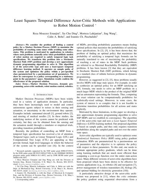
V. CASE STUDY
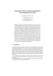
In this section we apply our algorithm to control a robot
moving in a square-shaped mission environment, which is
partitioned into 2500 smaller square regions (a 50 × 50 grid)
as shown in Fig. 1. We model the motion of the robot in the
environment as an MDP: each region corresponds to a state
of the MDP, and in each region (state), the robot can take
the following control primitives (actions): “North”, “East”,
“South”, “West”, which represent the directions in which the
robot intends to move (depending on the location of a region,
some of these actions may not be enabled, for example, in
the lower-left corner, only actions “North” and “East” are
enabled). These control primitives are not reliable and are
subject to noise in actuation and possible surface roughness
in the environment. Thus, for each motion primitive at a
region, there is a probability that the robot enters an adjacent
region.
We label the region in the south-west corner as the
initial state. We marked the regions located at the other
three corners as the set of goal states as shown in Fig. 1.
We assume that there is a set of unsafe states X U in the
environment (shown in black in Fig. 1). Our goal is to find
the optimal policy that maximizes the probability of reaching
a state in X G (set of goal states) from the initial state (an
instance of an MRP problem).

X
X
otherwise. Note that the availability of control actions at a
state is limited for the states at the boundary. For example,
at the initial state, which is at the lower-left corner, the set of
available actions is {u 1 , u 2 }, corresponding to “North” and
“East”, respectively. If an action u i is not available at state
x, we set a i (θ) = 0, which means that µ θ (u i |x) = 0.
Note that a i (θ) is defined to be the combination of the
expected safety score of the next state applying control u i ,
and the expected improved progress score from the current
state applying u i , weighted by θ 1 and θ 2 . The RSP is then
given by
a i (θ)
µ θ (u i |x) = ∑ 4
i=1 a i(θ) . (12)
O
Fig. 1. View of the mission environment. The initial region is marked by
o, the goal regions by x, and the unsafe regions are shown in black.
A. Designing an RSP
To apply the LSTD Actor-Critic algorithm, the key step is
to design an RSP µ θ (u|x). In this case study, we define the
RSP to be an exponential function of two scalar parameters
θ 1 and θ 2 , respectively. These parameters are used to provide
a balance between safety and progress from applying the
control policy.
For each pair of states x i , x j ∈ X, we define d(x i , x j )
as the minimum number of transitions from x i and x j . We
denote x j ∈ N(x i ) if and only if d(x i , x j ) ≤ r n , where r n
is a fixed integer given apriori. If x j ∈ N(x i ), then we say
x i is in the neighborhood of x j , and r n represents the radius
of the neighborhood around each state.
For each state x ∈ X, the safety score s(x) is defined as
the ratio of the safe neighbouring states over all neighboring
states of x. To be more specific, we define
∑
y∈N(x)
s(x) =
I s(y)
(10)
|N(x)|
where I s (y) is an indicator function such that I s (y) = 1
if and only if y ∈ X \ X U and I s (y) = 0 if otherwise. A
higher safety score for the current state of robot means it
is less likely for the robot to reach an unsafe region in the
future.
We define the progress score of a state x ∈ X as
d g (x) := min y∈XG d(x, y), which is the minimum number
of transitions from x to any goal region. We can now propose
the RSP policy, which is a Boltzmann policy as defined in
(1). Note that U = {u 1 , u 2 , u 3 , u 4 }, which corresponds to
“North”, “East”, “South”, and “West”, respectively. We first
define
a i (θ) = F i (x)e θ1E{s(f(x,ui))}+θ2E{dg(f(x,ui))−dg(x)} ,
(11)
where θ := (θ 1 , θ 2 ), and F i (x) is an indicator function such
that F i (x) = 1 if u i is available at x i and F i (x) = 0 if
X
We note that Assumption B holds for the proposed RSP.
Moreover, Assumption A also holds, therefore Theorem II.1
holds for this RSP.
B. Generating transition probabilities
To implement the LSTD Actor-Critic algorithm, we first
constructed the MDP. As mentioned above, this MDP represents
the motion of the robot in the environment where each
state corresponds to a cell in the environment (Fig. 1). To
capture the transition probabilities of the robot from a cell
to its adjacent one under an action, we built a simulator.
The simulator uses a unicycle model (see, e.g., [19]) for
the dynamics of the robot with noisy sensors and actuators.
In this model, the motion of the robot is determined by specifying
a forward and an angular velocity. At a given region,
the robot implements one of the following four controllers
(motion primitives) - “East”, “North”, “West”, “South”. Each
of these controllers operates by obtaining the difference
between the current heading angle and the desired heading
angle. Then, it is translated into a proportional feedback
control law for angular velocity. The desired heading angles
for the “East”, “North”, “West”, and “South” controllers are
0 ◦ , 90 ◦ , 180 ◦ , and 270 ◦ , respectively. Each controller also
uses a constant forward velocity. The environment in the
simulator is a 50 by 50 square grid as shown in Fig. 1. To
each cell of the environment, we randomly assigned a surface
roughness which affects the motion of the robot in that cell.
The perimeter of the environment is made of walls, and when
the robot runs to them, it bounces with the mirror-angle.
To find the transition probabilities, we performed a total of
5000 simulations for each controller and state of the MDP. In
each trial, the robot was initialized at the center of the cell,
and then an action was applied. The robot moved in that
cell according to its dynamics and surface roughness of the
region. As soon as the robot exited the cell, a transition was
encountered. Then, a reliable center-converging controller
was automatically applied to steer the robot to the center
of the new cell. We assumed that the center-converging
controller is reliable enough that always drives the robot
to the center of the new cell before exiting it. Thus, the
robot always started from the center of a cell. This makes
the process Markov (the probability of the current transition
depends only the control and the current state, and not on

eachability probability
1
0.8
0.6
0.4
0.2
0
0 200 400 600 800 1000 1200 1400 1600
iteration
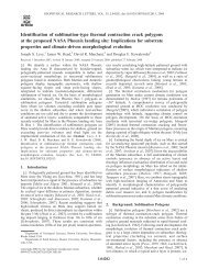
Fig. 2. The dashed line represents the optimal solution (the maximal
reachability probability) and the solid line represents the exact reachability
probability for the RSP as a function of the number of iterations applying
the proposed algorithm.
the history up to the current state). We also assumed perfect
observation at the boundaries of the cells.
It should be noted that, in general, it is not required to
have all the transition probabilities of the model in order
to apply the LSTD Actor-Critic algorithm, but rather, we
only need transition probabilities along the trajectories of the
system simulated while running the algorithm. This becomes
an important advantage in the case where the environment
is large and obtaining all transition probabilities becomes
infeasible.
C. Results
We first obtained the exact optimal policy for this problem
using the methods described in [2], [5]. The maximal
reachability probability is 99.9988%. We then used our
LSTD actor-critic algorithm to optimize with respect to θ
as outlined in Sec. III and IV.
Given θ, we can compute the exact probability of reaching
X G from any state x ∈ X applying the RSP µ θ by solving
the following set of linear equations
p θ (x) = ∑ u∈U
µ θ (u|x) ∑ y∈X
p(y|x, u)p θ (y),
for all x ∈ X \ (X U ∪ X G ) (13)
such that p θ (x) = 0 if x ∈ X U and p θ (x) = 1 if x ∈ X G .
Note that the equation system given by (13) contains exactly
|X| − |X U | − |X G | number of equations and unknowns.
We plotted in Fig. 2 the reachability probability of the
RSP from the initial state (i.e., p θ (x 0 )) against the number
of iterations in the actor-critical algorithm each time θ
is updated. As θ converges, the reachability probability
converges to 90.3%. The parameters for this examples are:
r n = 2, λ = 0.9, D = 5 and the initial θ is (50, −10). We
use (8) for β k with c = 0.05.
VI. CONCLUSION
We considered the problem of finding a control policy for a
Markov Decision Process (MDP) to maximize the probability
of reaching some states of the MDP while avoiding some
other states. We presented a transformation of the problem
into a Stochastic Shortest Path (SSP) MDP and developed a
new approximate dynamic programming algorithm to solve
this class of problems. The algorithm operates on a samplepath
of the system and optimizes the policy within a prespecified
class parameterized by a parsimonious set of parameters.
Simulation results confirm the effectiveness of the
proposed solution in robot motion planning applications.
REFERENCES
[1] S. Temizer, M. Kochenderfer, L. Kaelbling, T. Lozano-Pérez, and
J. Kuchar, “Collision avoidance for unmanned aircraft using Markov
decision processes.”
[2] M. Lahijanian, J. Wasniewski, S. B. Andersson, and C. Belta, “Motion
planning and control from temporal logic specifications with probabilistic
satisfaction guarantees,” in IEEE Int. Conf. on Robotics and
Automation, Anchorage, AK, 2010, pp. 3227 – 3232.
[3] R. Alterovitz, T. Siméon, and K. Goldberg, “The stochastic motion
roadmap: A sampling framework for planning with Markov motion
uncertainty,” in Robotics: Science and Systems. Citeseer, 2007.
[4] C. Baier, J.-P. Katoen, and K. G. Larsen, Principles of Model Checking.
MIT Press, 2008.
[5] X. Ding, S. Smith, C. Belta, and D. Rus, “LTL control in uncertain
environments with probabilistic satisfaction guarantees,” in IFAC,
2011.
[6] J. Peters and S. Schaal, “Policy gradient methods for robotics,”
in Proceedings of the 2006 IEEE/RSJ International Conference on
Intelligent Robots and Systems, 2006.
[7] K. Samejima and T. Omori, “Adaptive internal state space construction
method for reinforcement learning of a real-world agent,” Neural
Networks, vol. 12, pp. 1143–1155, 1999.
[8] H. Berenji and D. Vengerov, “A convergent Actor-Critic-based FRL
algorithm with application to power management of wireless transmitters,”
IEEE Transactions on Fuzzy Systems, vol. 11, no. 4, pp.
478–485, 2003.
[9] “Actor-critic models of reinforcement learning in the basal ganglia:
From natural to artificial rats,” Adaptive Behavior, vol. 13, no. 2, pp.
131–148, 2005.
[10] G. Gajjar, S. Khaparde, P. Nagaraju, and S. Soman, “Application
of actor-critic learning algorithm for optimal bidding problem of a
GenCo,” IEEE Transactions on Power Engineering Review, vol. 18,
no. 1, pp. 11–18, 2003.
[11] V. R. Konda and J. N. Tsitsiklis, “On actor-critic algorithms,” SIAM
Journal on Control and Optimization, vol. 42, no. 4, pp. 1143–1166,
2003.
[12] S. Bradtke and A. Barto, “Linear least-squares algorithms for temporal
difference learning,” Machine Learning, vol. 22, no. 2, pp. 33–57,
1996.
[13] V. R. Konda, “Actor-critic algorithms,” Ph.D. dissertation, MIT, Cambridge,
MA, 2002.
[14] D. Bertsekas and S. Ioffe, “Temporal differences-based policy iteration
and applications in neuro-dynamic programming,” LIDS REPORT,
Tech. Rep. 2349, 1996, mIT.
[15] J. Peters and S. Schaal, “Natural actor-critic,” Neurocomputing,
vol. 71, pp. 1180–1190, 2008.
[16] D. Bertsekas, Dynamic Programming and Optimal Control. Athena
Scientific, 1995.
[17] R. S. Sutton and A. G. Barto, Reinforcement Learning: An Introduction.
MIT Press, 1998.
[18] R. M. Estanjini, X. C. Ding, M. Lahijanian, J. Wang, C. A. Belta,
and I. C. Paschalidis, “Least squares temporal difference actor-critic
methods with applications to robot motion control,” 2011, available at
http://arxiv.org/abs/1108.4698.
[19] S. LaValle, Planning algorithms. Cambridge University Press, 2006.