Robot learning for ball bouncing
Robot learning for ball bouncing
Robot learning for ball bouncing

You also want an ePaper? Increase the reach of your titles
YUMPU automatically turns print PDFs into web optimized ePapers that Google loves.
<strong>Robot</strong> <strong>learning</strong> <strong>for</strong> <strong>ball</strong> <strong>bouncing</strong><br />
Denny Dittmar<br />
Denny.Dittmar@stud.tu-darmstadt.de<br />
Bernhard Koch<br />
Bernhard.Koch@stud.tu-darmstadt.de<br />
Abstract<br />
For robots automatically <strong>learning</strong> to solve a<br />
given task is still an hard job. Many real<br />
world challenges consist of complex movement,<br />
which has to be done in coordination<br />
with other objects or persons in order<br />
to achieve a required per<strong>for</strong>mance on a given<br />
task. In order <strong>for</strong> robots to be able to correctly<br />
behave in such environments it is important<br />
to use efficient controlling and <strong>learning</strong><br />
algorithms that can cope with high dimensional<br />
action spaces and achieve good results<br />
after a relatively short time using only<br />
indirect feedback of the per<strong>for</strong>mance of the<br />
robot, a so called reward. In this paper<br />
we compare two controlling approaches with<br />
specific <strong>learning</strong> parameters in order to per<strong>for</strong>m<br />
complex movements of an robot arm<br />
with seven DOFs and apply both of them to<br />
a <strong>learning</strong> algorithms. The task that has to<br />
be solved is to produce a stable <strong>bouncing</strong> of<br />
a <strong>ball</strong> with paddle as the end-effector of a<br />
manipulator. The first controlling approach<br />
tries to control the endeffector by defining<br />
and following a smooth polynomial trajectory<br />
in each step of the task. The second approach<br />
is to use Rhythmic Movement Primitives or<br />
RDMPs <strong>for</strong> short. For the <strong>learning</strong> algorithm<br />
we use the PoWER method.<br />
1 Introduction<br />
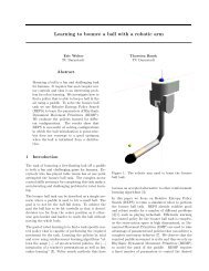
The task <strong>for</strong> the robot arm is to continuously bounce<br />
an free-floating <strong>ball</strong> on a racket attached to its endeffector<br />
<strong>for</strong> . As an additional difficulty there is a<br />
damping of the <strong>ball</strong> every time it hits the racket. To<br />
solve this task it is required to have a fast and precise<br />
controlling of the endeffector to an fast moving<br />
Preliminary work. Under review by AISTATS 2012. Do<br />
not distribute.<br />
<strong>ball</strong> which can only be controlled at each hit with the<br />
rack. Thus this task can be considered as non-trivial.<br />
Solving this task efficiently is an interesting research<br />
topic as it requires fast <strong>learning</strong> in complex mostly uncontrolled<br />
environments. To calculate the movement<br />
of the arm so it can hit the <strong>ball</strong> with the best trajectory<br />
is done through two different approaches. The<br />
first approach is a handcrafted controller using more<br />
complex expert knowledge of the whole task to calculate<br />
desired states of the racket at certain times and<br />
cover these states by smooth polynomial trajectories.<br />
The second approach is to use RDMPs to create an<br />
rhythmic movement which is able to reliably hit the<br />
<strong>ball</strong> so that we are able to bounce it. The per<strong>for</strong>mance<br />
of both approaches is initially bad especially<br />
<strong>for</strong> the RDMP approach as they require parameters to<br />
be <strong>learning</strong> <strong>for</strong> each specific task. So as an <strong>learning</strong> algorithm<br />
we are using the PoWER method as it showed<br />
the best results in comparison to other methods such<br />
as eNAC or RWR [KP11].<br />
2 Movement<br />
For moving the racket mounted to the endeffector of<br />
the arm we have chosen to compare two completely<br />
different approaches. This is done to compare an general<br />
framework <strong>for</strong> controlling the movement of robots<br />
such as RDMPs with an handcrafted policy which is<br />
using expert knowledge of the task.<br />
2.1 Controlling using smooth polynomial<br />
trajectories<br />
In this controlling approach at the beginning of each<br />
new <strong>bouncing</strong> step, that is at the beginning of the task<br />
and every time the racket hits the <strong>ball</strong>, desired values<br />
<strong>for</strong> the position, velocity and orientation are chosen<br />
<strong>for</strong> the next moment, when the racket hits the <strong>ball</strong>, in<br />
order to get an optimal behavior of the <strong>ball</strong>, that is a<br />
desired <strong>ball</strong> velocity, after the racket has hit the <strong>ball</strong>.<br />
Since there are many possibilites <strong>for</strong> the next hit position,<br />
these are restricted to lie on a imaginary 2-dplane,<br />
which is predefined by a height. Together with<br />
the current <strong>ball</strong> velocity it can be computed, where
Manuscript under review by AISTATS 2012<br />
the <strong>ball</strong> hits this plane next. This position then is desired<br />
to be the position, where the racket and the <strong>ball</strong><br />
should collide.<br />
As <strong>for</strong> the hit positions, there might also be many different<br />
velocities of the <strong>ball</strong>, that could result from the<br />
hit and so the velocities have to be restricted, too. The<br />
desired velocitiy of the <strong>ball</strong> is chosen, such that the<br />
next collision of the <strong>ball</strong> with the racket lies in an area,<br />
where the end-effector has much degrees of freedom<br />
with corresponding buffers <strong>for</strong> all these. Ideally this<br />
would be somewhere in the middle of the space that<br />
can be reached by the end-effector easily. This desired<br />
point was set by a <strong>learning</strong> <strong>learning</strong> parameter(Θ 1 )<br />
that set the y-value of the point with z given by the<br />
plane height and x = 0. To achieve a good resulting<br />
<strong>ball</strong> velocity that should have a low deviation to the<br />
desired <strong>ball</strong> velocity after the collision it is necessary<br />
to make sure that the paddle has an appropriate velocity<br />
and orientation, when it collides with the <strong>ball</strong>.<br />
This values also depend on the velocity the <strong>ball</strong> hits<br />
the paddle with.<br />
The orientation of the racket at the hit is chosen, such<br />
that both the velocity the <strong>ball</strong> hits the racket with and<br />
the desired velocity only possibly differ in normal direction<br />
of the paddle corresponding to reflection law<br />
assuming that the racket rests, i.e. has no zero velocity,<br />
and there is no damping etc... To compensate this<br />
velocity difference in normal direction and to take care<br />
of damping of unknown size the racket velocity in this<br />
direction is set to a value, such that the following chosen<br />
model equation holds <strong>for</strong> all these 1-dimensional<br />
velocities in racket normal direction:<br />
v <strong>ball</strong>out = v racket + d(v racket − v <strong>ball</strong>in ), (1)<br />
with d as damping. Thus it follows <strong>for</strong> the desired<br />
setting of the racket velocity:<br />
v racket = v <strong>ball</strong>out + dv <strong>ball</strong>in<br />
1 + d<br />
(2)<br />
Since good values <strong>for</strong> d are a-priori not known, d here<br />
was choosen to be <strong>learning</strong> parameter(Θ 2 ) of this<br />
control method based on this given model.<br />
After the time and desired racket state at the next<br />
collision with the <strong>ball</strong> have been calculated, there<br />
has to be a movement of the racket that makes sure,<br />
that the racket has this desired state, when the <strong>ball</strong><br />
hits the plane again. In order to avoid controlling<br />
difficulties this movement is desired to have a smooth<br />
trajectory with steady velocity, and to try to return<br />
to an basis point under the plane in somewhere in the<br />
movement, such that the racket has the possibility to<br />
accelerate to a desired velocity be<strong>for</strong>e it hits the <strong>ball</strong>.<br />
That means there are 3 given points of the trajectory,<br />
namely starting state, some intermediate basis state<br />
and the end state, where the racket should hit the<br />
<strong>ball</strong>.<br />
One possibility <strong>for</strong> such a smooth trajectory are<br />
linked polynomials, that are used in this approach.<br />
They were used by finding 2 polynomials, such that<br />
the first one goes from the current starting state<br />
through the intermediate basis state and the second<br />
from the intermediate basis state to the end state<br />
with the desired velocities. The polynomials also wer<br />
constraint to have equal velocities at the basis point,<br />
where they are connected. This desired velocity at the<br />
basis point was chosen such that it is directed to the<br />
desired collision point. The amount of the velocity<br />
was not fixed and instead used as settable <strong>learning</strong><br />
parameter(Θ 3 ) together with the ratio of the time<br />
amounts of both trajectories(Θ 4 ), which have to sum<br />
up to the remaining time until the next collision.<br />
Furthermore it is much more convenient to represent<br />
this desired states of the racket not in the task space,<br />
but in the joint space and to define the trajectory<br />
there instead. One heavy advantage of doing so is that<br />
<strong>for</strong> controlling it is not necessary to call an inverse<br />
kinematics method all time to find the corresponding<br />
joint configuration <strong>for</strong> current task state given by<br />
the trajectory at this moment. Instead the inverse<br />
kinematics method is only called three times per step<br />
in order to get the joint states <strong>for</strong> the desired start<br />
point, the basis point and end points of the resulting<br />
trajectory.<br />
Since <strong>for</strong> both of the 2 linked trajectories it must hold<br />
that they start at some desired start point and end at<br />
some desired end point with desired velocities there<br />
are <strong>for</strong> each trajectory 4 constraints <strong>for</strong> each joint<br />
given by its angle and angle velocity at the beginning<br />
and at the end of the trajectory. Thus a polynomiala<br />
of degree 3 are sufficient to represent these one of<br />
both trajectories <strong>for</strong> each joint. Such polynomials<br />
have been used <strong>for</strong> this controlling method.<br />
2.2 RDMPs - Rhythmic dynamic movement<br />
primitives<br />
To create complex movements <strong>for</strong> robots dynamic<br />
movement primitives, DMPs <strong>for</strong> short, have been<br />
shown to be quite versatile [SMI07]. With them it<br />
is possible to create complex non-linear trajectories<br />
which can be easily adapted to different goal positions<br />
and can be scaled with the time to create slower or<br />
faster movements. As the movement we need to be<br />
able to bounce the <strong>ball</strong> is an rhythmic one we use<br />
the rhythmic variation of the DMPs [SPNI04]. Rhythmic<br />
dynamic movement primitives or RDMPs <strong>for</strong> short
Manuscript under review by AISTATS 2012<br />
consist of three equations. An trans<strong>for</strong>mation system,<br />
τż = α z (β z (g − y) − z), τẏ = z + f (3)<br />
where g is the setpoint of the oscillation of the rhythmic<br />
movement, α z and β z are time constants, τ is the<br />
temporal scaling factor to speed up or slow down the<br />
movement and y, ẏ are the desired position and velocity.<br />
The second equation is the canonical system, in<br />
this case an phase-amplitude oscillator,<br />
τṙ = α r (A − r), τ ˙φ = 1 (4)<br />
where r is the amplitude, A the desired amplitude and<br />
φ the phase of the oscillator. The last equation needed<br />
is the non-linear function<br />
f(r, φ) =<br />
N∑<br />
ψ i ∗ wi<br />
T ∗ v<br />
i=1<br />
v = [ r ∗ cos φ<br />
with (5)<br />
N∑<br />
ψ i<br />
i=1<br />
r ∗ sin φ ] T<br />
ψ i = exp((−h i (φ mod 2π) − c i ) 2 )<br />
and<br />
where the w i are the weights which essentially describe<br />
the trajectory. So the <strong>learning</strong> parameters <strong>for</strong> these<br />
equations are the τ <strong>for</strong> the time scaling and the weights<br />
w i <strong>for</strong> the actual trajectory. For our setup we only use<br />
one RDMP and have there<strong>for</strong>e only one controllable<br />
DOF in the arm. The reason <strong>for</strong> this is so that we<br />
have fewer parameters which need to be learned and<br />
there<strong>for</strong>e an smaller <strong>learning</strong> space.<br />
3 Learning methods<br />
Both approaches described in this paper need to be<br />
adapted to specific movements of the <strong>ball</strong>. For example<br />
an slow moving <strong>ball</strong> requires slower movements of<br />
the arm in comparison to an fast moving <strong>ball</strong>. This is<br />
especially true when the initial position and initial velocity<br />
of the <strong>ball</strong> is changing with each iteration of the<br />
simulation. This adaption is done through <strong>learning</strong> parameters<br />
which need to be automatically fitted to the<br />
task. For this comparison we are using the PoWER<br />
<strong>learning</strong> algorithm.<br />
3.1 PoWER - Policy <strong>learning</strong> by Weighting<br />
Exploration with the Returns<br />
This <strong>learning</strong> algorithm is based on updating the <strong>learning</strong><br />
parameters by doing multiple rollouts of the policy<br />
which should be learned with the same <strong>learning</strong> parameters<br />
each time disturbed by an small exploration<br />
value. The rewards <strong>for</strong> each of these rollouts will then<br />
be sorted and the X best rollouts will then be used<br />
to calculate the parameters <strong>for</strong> the next iteration of<br />
rollouts. This calculation is done by weighting the exploration<br />
values which were applied to the parameters<br />
<strong>for</strong> each rollout with the result of the Qsat and the<br />
Wst function and then multiplying it with its inverse<br />
but without the exploration values. The Qsat function<br />
takes the start state of the simulation, the action<br />
taken by the policy and the resulting ending state of<br />
the simulation as an input and uses this in<strong>for</strong>mation<br />
to provide an evaluation on how good this action was<br />
given the states of the simulation. The Wst function<br />
is used to provide extra weight to certain states of<br />
the simulation making it possible to provide an boost<br />
<strong>for</strong> parameters of the policy which resulted in winning<br />
state or to punish when the last state of the simulation<br />
was especially bad. This algorithm is then run either<br />
until the parameters have converged to an optimum or<br />
until an maximum number of iterations is reached. We<br />
have chosen this method <strong>for</strong> <strong>learning</strong> the parameters<br />
as it per<strong>for</strong>med best when compared to other <strong>learning</strong><br />
methods such as eNAC and RWR [KP11]. It also<br />
treats the policy as an black box and does not need<br />
to know how it works or what it does at it operates<br />
entirely on the rewards and Qsat and Wst functions,<br />
making it perfectly suited to compare different policies<br />
against each other. But it cannot provide any guarantee<br />
that it will converge to the global maximum of the<br />
rewards and there<strong>for</strong>e not to the best possible values<br />
<strong>for</strong> the policy.<br />
Algorithm 1 PoWER - Policy <strong>learning</strong> by Weighting<br />
Exploration with the Returns<br />
Precondition: intial policy parameters Φ<br />
function PoWER(Φ)<br />
repeat<br />
<strong>for</strong> r ≤ mR do<br />
reward r = policy(Φ k + exploration r )<br />
end <strong>for</strong><br />
Φ k+1 = Φ k +<br />
until Φconverged<br />
return Φ optimal<br />
end function<br />
4 Comparison<br />
mR ∑<br />
Qsat t∗W st t∗exploration t<br />
t=1<br />
mR ∑<br />
Qsat t∗W st t<br />
t=1<br />
We compare both approaches by providing them with<br />
the same initial state of the simulation. In this initial<br />
state the <strong>ball</strong> is placed directly above racket with zero<br />
velocity. We are also using the previously described<br />
PoWER <strong>learning</strong> algorithm to learn both policies in<br />
order to give them the same conditions. Initially we<br />
wanted to makes them easily comparable by using the<br />
same reward function <strong>for</strong> both approaches but as we
Manuscript under review by AISTATS 2012<br />
cannot do the comparison cause of the poor per<strong>for</strong>mance<br />
achieved through the RDMP approach we decided<br />
to use different reward <strong>for</strong> each approach. Both<br />
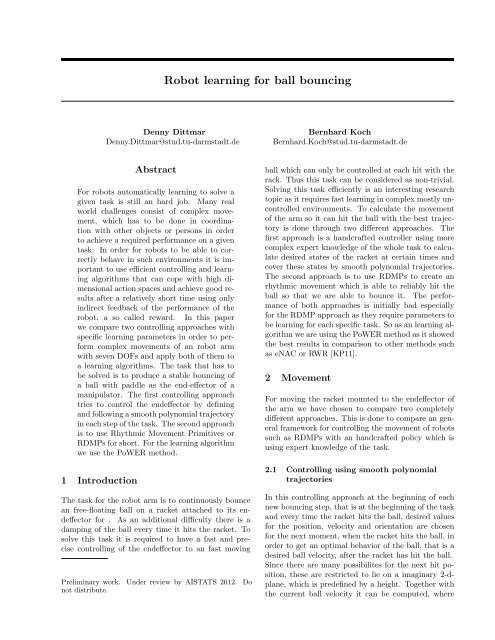
rewards are described below. Figure 1 shows the <strong>learning</strong><br />
curve of the RDMP approach over 100 iterations<br />
with 15 rollouts in each iteration. The blue line is the<br />
mean of the 10 best rollouts in that iteration while the<br />
shaded area shows the minimum/maximum reward.<br />
The reward is calculated by taking the difference of<br />
the <strong>ball</strong> velocity and an ideal velocity at each hit with<br />
the racket. The ideal velocity points straight up to<br />
make sure to keep the <strong>ball</strong> over the racket. So thee<br />
more the actual <strong>ball</strong> velocity differs from the ideal one<br />
at each hit the reward decreaes.<br />
Figure 2: Learning curve <strong>for</strong> the polynomial trajectories<br />
approach over 100 iterations showing the highest<br />
number of hits achived until this iteration<br />
Figure 1: Learning curve <strong>for</strong> the RDMP approach of<br />
100 iterations using 15 rollouts per iteration<br />
As we had several problems with the RDMP approach<br />
an comparison with the other approach does not make<br />
much sense. As figure 1 shows the <strong>learning</strong> curve stays<br />
at an pretty low level <strong>for</strong> all iterations. We assume that<br />
this is caused by either just an bad reward function<br />
or by an incomplete or wrong understanding of the<br />
behavior of RDMPs.<br />
In figure 2 you can see the <strong>learning</strong> curve <strong>for</strong> the approach<br />
using polynomial trajectories. As we cannot<br />
do an comparison cause of the bad per<strong>for</strong>mance of<br />
our RDMP approach we have used an different reward<br />
function just based on the number hits. This approach<br />
improves quite nicely until it reaches an local optima<br />
at nine hits per iteration.<br />
5 Conclusion<br />
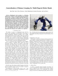
In this paper we tried to compare two very different<br />
approaches <strong>for</strong> calculating the best movement <strong>for</strong> an<br />
racket attached to end of an seven DOF robot arm<br />
to continuously bounce an free-floating <strong>ball</strong>. The first<br />
method we used was to use our expert knowledge of<br />
the specific task to calculate the best trajectory to hit<br />
the <strong>ball</strong>. Such an approach is only feasible <strong>for</strong> smaller<br />
tasks as it is very complex to create such an policy.<br />
Another disadvantage of that approach is that it is<br />
limited to solving only that specific task. The second<br />
approach we used and compared to the first one<br />
was to use rhythmic dynamic movement primitives as<br />
they are an general framework <strong>for</strong> movement which<br />
can work in an multitude of different tasks. As such<br />
they are already used in various other tasks [Sch] and<br />
can be extended to also avoid obstacles [hPHPS]. For<br />
both algorithms we used the same reward function and<br />
the same <strong>learning</strong> algorithm, namely the PoWER algorithm.<br />
Because we had various problems with both<br />
approaches we failed to do an good comparison of them<br />
as both of their per<strong>for</strong>mances and their <strong>learning</strong> curves<br />
are suboptimal as shown in 1. The next steps would<br />
be to improve the <strong>learning</strong> of both approaches and to<br />
introduce multiple RDMPs to enable more than one<br />
controllable DOF.<br />
References<br />
[hPHPS] Dae hyung Park, Heiko Hoffmann, Peter<br />
Pastor, and Stefan Schaal. Movement reproduction<br />
and obstacle avoidance with dynamic<br />
movement primitives and potential<br />
fields. In in IEEE International Conference<br />
on Humanoid <strong>Robot</strong>ics.<br />
[KP11] J. Kober and J. Peters. Policy search <strong>for</strong><br />
motor primitives in robotics. (1-2):171–203,<br />
2011.<br />
[Sch] Stefan Schaal. Dynamic movement primitivesa<br />
framework <strong>for</strong> motor control in hu-
Manuscript under review by AISTATS 2012<br />
mans and humanoid robotics.<br />
[SMI07] Stefan Schaal, Peyman Mohajerian, and<br />
Auke Ijspeert. A.j.: Dynamics systems vs.<br />
optimal control a unifying view. In Progress<br />
in Brain Research, pages 425–445, 2007.<br />
[SPNI04] Stefan Schaal, Jan Peters, Jun Nakanishi,<br />
and Auke Ijspeert. Learning movement<br />
primitives. In International Symposium<br />
on <strong>Robot</strong>ics Research (ISRR2003. Springer,<br />
2004.