Directed Search with Endogenous Search Effort.
Directed Search with Endogenous Search Effort.
Directed Search with Endogenous Search Effort.

Create successful ePaper yourself
Turn your PDF publications into a flip-book with our unique Google optimized e-Paper software.
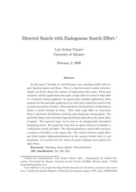
<strong>Directed</strong> <strong>Search</strong> <strong>with</strong> <strong>Endogenous</strong> <strong>Search</strong> E¤ort. <br />
Lari Arthur Viianto y<br />
University of Alicante<br />
February 2, 2009<br />
Abstract<br />
In this paper I develop an urn-ball game type matching model <strong>with</strong> exante<br />
identical agents and …rms. This is a directed search market structure.<br />
Agents can freely choose the amount of applications they make. Firms post<br />
vacancies, receive applications and make a single take-it-or-leave-it wage o¤er<br />
to a randomly chosen applicant. As agents make multiple applications, …rms<br />
compete for the particular applicant as in a …rst-price sealed-bid auction <strong>with</strong><br />
an unknown number of biders. Miscoordiantion and asymmetry of information<br />
induce a mixed strategy by …rms. They make wage o¤ers as extractions<br />
from a continuous distribution, inducing wage dispersion among agents. The<br />
particular shape of the obtained wage distribution depends on the search e¤ort<br />
of agents. The expected wage can be seen as an endogenously determined<br />
bargaining power. The particular wage that an agent receives is stochastic, a<br />
combination of luck and e¤ort. The miscoordination in search e¤ort produces<br />
a negative externality on the agents side. The relation between search e¤ort<br />
and labor market tightness(understood as the vacancy/worker ratio) is not<br />
monotonic. It is positive for low values of market tightness and negative for<br />
high values.<br />
Keywords: Matching, Labor Market, <strong>Directed</strong> <strong>Search</strong>.<br />
JEL classi…cation: J31, J65, D83<br />
Address for correspondence: Lari Arthur Viianto, Dpto. Fundamentos del Analisis Economico,<br />
Universidad de Alicante, Carretera de San Vicente, E-03069, Alicante, Spain. E-Mail:<br />
lariarthur@merlin.fae.ua.es<br />
y I am indebted to my supervisor Iñigo Iturbe-Ormaetxe for his advice, comments and corrections.<br />
I thanks the Spanish Ministry of Education for …nancial support, FPU grant AP2003-0563.
1 Introduction<br />
One of the frictions present in labor markets is the matching process, a mechanism<br />
required to match …rms and workers. In most of the literature, the matching<br />
mechanism is just an exogenously imposed function describing the relation between<br />
market tightness and the number of matches. In most of these models, the search<br />
direction is not addressed and search e¤ort is absent. To address the search direction<br />
a description of the market structure is required. The urn-ball game induces such a<br />
market structure. In this set-up one of the sides of the market, typically the worker,<br />
initiates the process by making an initial contact <strong>with</strong> the other side, typically the<br />
…rm.<br />
However, in the standard urn-ball game, search e¤ort is not present since<br />
agents make a single application. Albrecht, Gautier and Vroman (2006, hereafter<br />
AGV) solve this question by allowing agents to make any number of applications.<br />
However, in their work the particular number of applications is an exogenous variable.<br />
1 The wage bargaining process, absent in the urn-ball game, becomes relevant.<br />
Since agents make more that one application they can receive more than one o¤er.<br />
What AGV propose is a wage posting set up where, in the case that more than one<br />
…rm chose the same applicant, they engage in a Bertrand competition for that particular<br />
applicant. Then, in equilibrium, …rms post the reservation wage. An agent<br />
<strong>with</strong> only one o¤er gets the reservation wage, since it does not induce Bertrand<br />
competition among …rms, while an agent <strong>with</strong> more than one o¤er gets the whole<br />
production value as a result of Bertrand competition. The result is a wage dispersion<br />
concentrated in two extreme cases. It also assumes that …rms have information<br />
about the number of o¤ers that agents receive. It implies losses for all …rms that<br />
make a match after a Bertrand competition.<br />
This paper has two main di¤erences <strong>with</strong> the work by AVG. The wage bargaining<br />
mechanism and the explicit endogeneity of search e¤ort. I assume that …rms do not<br />
post wages, only vacancies. After receiving applications, …rms make a single, takeit-or-leave-it,<br />
wage o¤er to a randomly chosen applicant.<br />
Firms compete to be<br />
1<br />
AGV endogenaizes the search e¤ort in section 5.1 as a robustness check. What they<br />
do is to look for a set of equilibrium values that sustain a particular equilibrium value of<br />
applications. Here I will solve directly the behavior of agents.<br />
1
the highest o¤er that the agent receives, <strong>with</strong>out information about the number of<br />
o¤ers received by the applicant. This turns out to be identical to a sealed …rst-price<br />
auction <strong>with</strong> an unknown number of bidders. The resulting wage o¤er distribution is<br />
continuous between the reservation wage and an upper-bound value that is strictly<br />
lower that the total value of production. This implies that a match yields always<br />
positive pro…ts. The shape of the wage distribution will depend both on labor<br />
market tightness and on search e¤ort. Intuitively, the expected wage can be seen as<br />
an endogenously determined bargaining power that depends on the search e¤ort of<br />
agents, while the highest o¤er that the agent receives will be an extraction from this<br />
distribution. The particular wage that the agent obtains is, therefore, a combination<br />
of luck and e¤ort. E¤ort induces the shape of the distribution while luck determines<br />
the particular value of the extracted wage.<br />
The relation obtained between market tightness and search e¤ort is not monotonic.<br />
It is positive for low values of market tightness and negative for high values. This<br />
result implies that an increase in the number of existing job vacancies induces an<br />
increase(decrease) in the search e¤ort when the number of vacancies is low(high).<br />
In the model there are severe problems of coordination and asymmetry of information.<br />
These problems will produce negative externalities. The most tractable<br />
externality is related to the miscoordination of agents regarding the number of applications<br />
they send. The equilibrium result shows that agents send too many applications.<br />
The excessive amount of applications produces a negative externality on<br />
the expected return of agents, due to excessive competition. A model where agents<br />
can coordinate in the number of applications is easy to implement and, therefore,<br />
the value of the negative externality can be measured comparing both results.<br />
The model accepts a wide set of extensions, as introducing heterogeneity in one<br />
(or both) sides of the market or additional wage o¤er rounds.<br />
The rest of the paper is organized as follows. In section 2, I solve the static<br />
model as a one shoot game. Section 3 present the results relative to the externality<br />
produced by the miscoordination of agents. Section 4 presents a robustness check<br />
including the free entry condition for …rms and a dynamic version of the model.<br />
2
Section 5 presents a set of extensions of the static model and section 6 concludes.<br />
2 Model<br />
I consider an economy where N agents are looking for a job and there are V posted<br />
job vacancies. Both agents and vacancies are homogeneous and both numbers are<br />
common knowledge. First …rms post vacancies, one per …rm. Agents observe the<br />
number of vacancies V and send an amount S of applications, I assume that they<br />
cannot apply twice to the same vacancy. Each application has a cost c for the<br />
agent. Once applications are made, …rms <strong>with</strong> at least one application choose one,<br />
at random, and make a wage o¤er W . The value of W and the identity of the chosen<br />
applicant are private information. Agents collect o¤ers and accept the highest one,<br />
provided that it exceeds the reservation wage w. 2 An accepted o¤er makes a match<br />
and the vacancy is ful…lled. Each ful…lled vacancy generates a value Q for the …rm.<br />
There are several coordination problems involved. Agents cannot coordinate in<br />
which …rms they make applications, neither in the number of applications. Firms<br />
cannot coordinate in which agents they make o¤ers or in the amount of the o¤er.<br />
There is asymmetry of information as …rms do not know the number of o¤ers that<br />
an agent has received, neither the value of particular o¤ers.<br />
I will use a symmetric equilibrium concept where homogeneous players behave<br />
identically. First I will solve all the probabilities involved in the matching process<br />
and then I will solve the model backwards. Then I will solve the wage o¤er decision<br />
of …rms and, …nally, the number of applications that agents wish to make.<br />
2.1 Probability construction<br />
In equilibrium all agents will make the same number S of applications. Since an<br />
agent sends S applications, a …rm has a probability S of receiving an application<br />
V<br />
<br />
S<br />
from a given agent and a probability 1<br />
V of not receiving it. It will not have any<br />
N.<br />
application <strong>with</strong> probability 1 A …rm receives at least one application <strong>with</strong><br />
2<br />
Or randomizes between the highest o¤ers if there is a tie.<br />
S<br />
V<br />
3
S N.<br />
probability 1 1<br />
V The total number of o¤ers made in the economy is equal to<br />
<br />
S N<br />
the number of …rms that receive at least one application, that is V 1 1 .<br />
V<br />
The probability that a particular application is successful is:<br />
O(S; V; N) =<br />
V<br />
<br />
1 1<br />
S<br />
V<br />
SN<br />
N<br />
<br />
. (1)<br />
For N large enough this expression can be approximated by:<br />
where = V N<br />
O(S; ) = 1<br />
describes the labor market tightness.<br />
e S=<br />
, (2)<br />
S<br />
An agent making S applications has a probability 1 (1 O(S; )) S of receiving<br />
at least one wage o¤er. Each worker <strong>with</strong> at least one wage o¤er makes a match.<br />
The total number of matches is: 3<br />
m(S; ) = N(1 (1 O(S; )) S ). (3)<br />
2.2 Firms wage o¤er<br />
Each …rm makes a single wage o¤er to a randomly chosen application. Firms will<br />
anticipate the number of applications made, and the behavior of the rest of the …rms.<br />
The …rm makes the wage o¤er that yields the highest expected pro…t, or randomize<br />
between the wages that yield the highest expected pro…t. The …rm chooses its o¤er<br />
among the set of wages W that yield the highest expected pro…t:<br />
W = arg max f(Q W ) F (W )g , (4)<br />
where (Q W ) is the pro…t if the wage is W and F (W ) is the probability that a<br />
wage o¤er of W is accepted.<br />
3<br />
This result anticipates that an o¤er is always higher than the reservation wage.<br />
4
The agents accepts a particular o¤er only if it is the highest one among all<br />
received o¤ers. This implies that F (W ) is equivalent to the cumulative distribution<br />
function of the highest o¤er received from other …rms. The …rm does not know the<br />
exact number of o¤ers that the agent has received, but it can construct F (W ) in<br />
order to compute the expected pro…t of a particular wage o¤er. Firms choose the<br />
wage o¤er in an, ex-ante, identical way. To be as general as possible I assume that<br />
the strategy space of …rms is B(W ), where B(W ) represents all possible cumulative<br />
distribution functions over W .<br />
Then F (W ) can be constructed as follows:<br />
F (w W ) = (1 O(S; )) S 1 + S P 1<br />
if B(W ) is continuous in W , or<br />
i=1<br />
<br />
S 1<br />
i O(S; ) i (1 O(S; )) S 1 i B(w W ) i ,<br />
(5)<br />
F (w W ) = F (w < W ) + S P 1<br />
i=1<br />
1<br />
i<br />
<br />
S 1<br />
i O(S; ) i (1 O(S; )) S 1 i B(w = W ) i , (6)<br />
if B(W ) has a discontinuity in W .<br />
This is identical to a sealed bid …rst-price auction <strong>with</strong> an unknown number of<br />
bidders, where all bidders value the good exactly the same. 4<br />
Next I describe the behavior of …rms in a set of lemmas.<br />
Lemma 2.1 Any wage o¤er must be higher or equal than the reservation wage w<br />
and lower or equal than the production value Q.<br />
Proof. Any o¤er lower than the reservation wage yields negative pro…ts as the<br />
probability of acceptance is zero. Then it is dominated by the reservation wage. Any<br />
o¤er higher than the production value yields negative pro…t so it is also dominated.<br />
4<br />
The exact number of bidders is unknown, but it is bounded by S.<br />
5
Lemma 2.2 The distribution B(W ) cannot have any discontinuity and, therefore,<br />
F (W ) has a unique discontinuity at the reservation wage, due to the probability that<br />
an agent has no other o¤er.<br />
Proof. If B(W ) has a discontinuity at some wage, this wage o¤er does not belong<br />
to W . An epsilon higher o¤er yields a higher expected pro…t since there is a<br />
discontinuity in F (W ) that increases drastically the probability of acceptance.<br />
The above results imply that F (W ) can be stated as<br />
XS 1 S 1<br />
F (W w) = (1 O(S; )) S 1 +<br />
O(S; ) i (1 O(S; )) S 1 i B(W w) i ,<br />
i<br />
i=1<br />
(7)<br />
that is equivalent to<br />
F (W ) = ((1 O(S; )) + O(S; )B(W )) S 1 . (8)<br />
It also implies that the probability that a …rm makes a particular wage o¤er is<br />
zero, that is, B(w = W ) = 0.<br />
Lemma 2.3 The lowest o¤er is the reservation wage w and the probability of acceptance<br />
is equal to the probability of having no other o¤er.<br />
Proof. If the reservation wage were not the lowest o¤er, the probability of acceptance<br />
of the lowest o¤er and the reservation wage would be the same. Then, to o¤er<br />
the reservation wage w yields a higher pro…t. As B(w = w) = 0, the reservation<br />
wage is accepted only if there is no other o¤er.<br />
Lemma 2.3 implies that:<br />
F (w) = (1 O(S; )) S 1 . (9)<br />
Lemma 2.4 The highest o¤ered wage w must be equal to Q (Q w)(1 O(S; )) S 1 .<br />
6
Proof. The expected pro…t is constant for all wages in the set W . The highest<br />
wage has probability one of acceptance and yields a pro…t (Q w). This pro…t must<br />
be equal to (Q w)(1 O(S; )) S 1 , the expected pro…t of o¤ering the reservation<br />
wage w.<br />
Lemma 2.5 If all …rms use the same distribution of wage o¤ers, then the domain<br />
of B(W ) must coincide <strong>with</strong> the domain of W , this domain must be connected,<br />
compact and must contain more than one value.<br />
Proof. Firms make o¤ers taking wages from the set W . A priori they can make<br />
o¤ers from di¤erent subsets since they are indi¤erent among wages in W . The<br />
…rst part of the lemma claims that all …rms must attach some probability to all<br />
wages in W . This is due to the construction of W that depends on F (W ) that,<br />
in turn, depends on B(W ). Observe that if W contains more than one value it<br />
must hold that (Q W )F (W ) is identical in all of them. Since F (W ) is a function<br />
<strong>with</strong>out discontinuities above w, then W must be connected. If there were two<br />
di¤erent subsets, any intermediate value will dominate them because it will give<br />
higher expected pro…t. 5 Then F (W ) must be strictly increasing for all values in W<br />
and, therefore, B(W ) must also be strictly increasing for all those values. The set is<br />
bounded because the wage o¤ers cannot be lower than w and cannot exceed w, and<br />
it is closed because both values are in the set. The set is connected, bounded and<br />
closed so it is compact. The set cannot be a singleton because o¤ering an epsilon<br />
higher wage will yield a higher pro…t.<br />
Lemma 2.5 implies that W is a connected set where:<br />
(Q W i ) F (W i ) = (Q W j )F (W j ) 8W i ; W j 2 W . (10)<br />
Since w 2 W and F (w) = (1 O(S; )) S 1 then:<br />
F (W ) = Q w<br />
Q W (1 O(S; ))S 1 for W 2 [w; w]. (11)<br />
5<br />
It has the same probability to be accepted than the lowest wage in the upper set that<br />
belongs to w but yields a higher pro…t.<br />
7
With this equation and using Equation(8), B(W ) can be written as:<br />
B(W ) = (1<br />
O(S; ))<br />
O(S; )<br />
Q<br />
Q<br />
w<br />
W<br />
1<br />
S 1<br />
1<br />
!<br />
. (12)<br />
The behavior of …rms is characterized by a continuous cumulative distribution<br />
function over a connected set of wages. Note that this implies wage dispersion among<br />
identical agents that make an identical number of applications, this dispersion does<br />
not require any exogenous random variable. The wage distribution is a result of the<br />
competition among …rms to hire a particular worker and of their lack of information.<br />
The number of o¤ers received by the worker is not known by …rms, so they will attach<br />
a positive probability to the event that they are making the only o¤er. To o¤er the<br />
reservation wage has a positive expected pro…t and all other o¤ers must yield the<br />
same expected pro…t. The competition among …rms is assumed to be restricted<br />
to a single take-it-or-leave-it o¤er. This assumption is sustained by the same lack<br />
of information. A …rm will not enter in to ex-post competition after a rejection,<br />
because it would be optimal for the agent to reject any o¤er in order to induce a<br />
wage increase. 6<br />
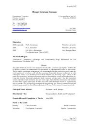
The …rms cumulative wage o¤er distribution, for Q = 1, = 1 and w = 0, has<br />
the following shape:<br />
6<br />
Any o¤er lower than the value of total production.<br />
8
Figure 1: CDF of wage o¤ers.<br />
Firms react to the number of applications that agents send. If agents send a<br />
single application, …rms will not have incentives to o¤er more than the reservation<br />
wage. The increase in the number of applications rises the probability that an agent<br />
has more that one o¤er. This drives the wage o¤er distribution closer to its limiting<br />
value. An increase in the number of applications moves to the right the upper bound<br />
of the distribution. The distribution related to a particular number of applications<br />
stochastically dominates all distributions corresponding to fewer applications.<br />
The wage o¤er distribution converges to the limiting distribution:<br />
lim B(W ) = 1 Q w<br />
S!1 ln Q W<br />
for W 2 [w; w] (13)<br />
If the agents send an in…nite number of applications the probability of receiving<br />
a particular number of applications can be expressed as a Poison distribution. This<br />
approach is followed by Halko, Kultti and Virrankoski (2008). Here I am interested<br />
in the problem related to the choice of search e¤ort. Agents will not make an in…nite<br />
number of applications.<br />
9
2.3 <strong>Search</strong> e¤ort<br />
Agents maximize the expected return corresponding to the number of applications<br />
S. They take into account the cost of applications and the behavior of the rest of<br />
the society. Agents observe the market tightness and give their best response to a<br />
scenario where the rest of agents make a …xed number of applications S.<br />
Firms o¤er wages according to B(W ) that is related to S. Agents are concerned<br />
about the highest o¤er they receive, since this will be the o¤er they will accept.<br />
Agents then compute H(W ), the cumulative distribution function of the highest<br />
o¤er received, that can be constructed as:<br />
H(w W ) =<br />
that is equivalent to:<br />
SX<br />
i=1<br />
S<br />
i<br />
<br />
O(S; ) i (1 O(S; )) S i B(w W ) i , (14)<br />
H(W ) = (1<br />
O(S; )) + O(S; )B(W ) S<br />
(1 O(S; )) S . (15)<br />
However this is not the wage of agents yet. Agents have an outside option.<br />
If they do not receive any o¤er, they earn the reservation wage. The cumulative<br />
distribution function of the wage associated to S applications is: 7<br />
R(W ) = (1 O(S; )) + O(S; )B(W ) S<br />
for W 2 [w; w]. (16)<br />
Plugging B(W ) in this function I get:<br />
S<br />
Q w<br />
R(W ) = (1 O(S; )) S S 1<br />
. (17)<br />
Q W<br />
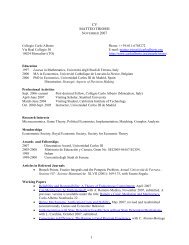
The distribution of the wage that agents perceive, for …xed S = 20, = 1, Q = 1,<br />
w = 0, is:<br />
7<br />
The return takes into account that the agent will receive the reservation wage if there<br />
are no o¤ers.<br />
10
Figure 2: Wage, taking as given the behaviour of the rest of the society.<br />
Here agents do not take into account the relation between their behavior and<br />
the behavior of the rest of the agents, they just take S as …xed. As in equilibrium<br />
all agent make S applications, the equilibrium cumulative distribution of the return<br />
looks like follows:<br />
Figure 3: Wage distribution.<br />
11
when agents take S as given, they believe that by increasing the number of applications<br />
they will, individually, face a distribution that stochastically dominates<br />
the distributions corresponding to fewer applications. In equilibrium the distributions<br />
cross each other, so there is no dominance. This is re‡ected in the negative<br />
externality related to the excessive number of applications in equilibrium.<br />
Agents choose S to maximize the expected return, taking as given the behavior<br />
of the rest of the society.<br />
The density function of the wage is:<br />
r(W ) =<br />
S<br />
S 1 1 O(S; ) S<br />
Q<br />
Q<br />
w<br />
W<br />
S<br />
S 1 1<br />
Q W . (18)<br />
The problem of the agents is to maximize the return, that is, the expected wage<br />
minus the cost of applications:<br />
Max<br />
S<br />
Q (Q w)(1<br />
Z<br />
O(S;)) S 1<br />
w<br />
W r(W )dW Sc. (19)<br />
This can be written as:<br />
Max<br />
S<br />
<br />
Q S(Q w)(1 O(S;))S 1 ((S 1)Q Sw)(1 O(S;)) S<br />
1+S S<br />
Sc. (20)<br />
This function has a unique maximum <strong>with</strong> respect to S.<br />
The …rst-order condition, once I impose the symmetry condition<br />
S = S is:<br />
<br />
(S 1) (1 O(S; )) S (Q w)O(S;)<br />
Q w S<br />
1 O(S;) S 1<br />
(ln(1 O(S; )) 1 ) = c. (21)<br />
Observe that in this expression, the term Q w S<br />
S 1<br />
makes the reservation<br />
wage more relevant than what it is generally assumed. It is usual to assume that<br />
the relevant variable is just the di¤erence between production and the reservation<br />
wage, so the reservation wage is set to zero. This simpli…cation cannot be done here<br />
12
unless the number of applications goes to in…nity. Still I can express the relevant<br />
variables as shares of the production, by setting Q = 1. 8<br />
Unfortunately, Expression21 , cannot be solved analytically, but it can be easily<br />
solved using a computer.<br />
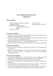
Fixing Q = 1, w = 0 and c a = 0:001; the optimal number of applications as a<br />
function of , has the following shape:<br />
Figure 4: Optimal number of applications as a function of .<br />
The optimal search e¤ort has not a monotonic relation <strong>with</strong> market tightness.<br />
For low values of market tightness the search e¤ort is increasing <strong>with</strong> while for<br />
high values it is decreasing. This implies a procyclical behavior in the low range of<br />
and a countercyclical behavior for high rates of . In this particular example the<br />
procyclical behavior is found for the most realistic values of . For those values, a<br />
decrease in , due to a decrease in the number of vacancies or to an increase in the<br />
number of agents, will decrease the search e¤ort. In this example, the countercyclical<br />
behavior is found for very high values of , where the number of vacancies is at least<br />
twice as high as the number of agents. Even when this seems unrealistic, this pattern<br />
8<br />
Many other variables, that are not considered in the model, can be easily included as<br />
changes in the existing set of variables. For example a linear wage tax can be included as<br />
a change the reservation wage to .<br />
<br />
w<br />
1 t<br />
13
can be found in some sectors. Mostly in sectors related to seasonal activities or <strong>with</strong><br />
low return unskilled activities.<br />
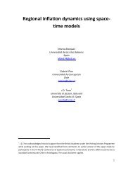
The expected return and wage, as a function of , are<br />
Figure 5: Expected wage and return.<br />
Here the expected wage is equivalent to the share of total production that agents<br />
expect to receive. This can be interpreted as an endogenous measure of the bargaining<br />
power of agents that depends on the market tightness . Changes in the<br />
market tightness will imply di¤erent bargaining powers. An increase in the number<br />
of agents looking for a job, for example an increase of unemployment, will harm the<br />
bargaining power of agents as it implies a decrease in .<br />
The particular wage that agents will receive is still stochastic, being the wage<br />
cumulative distribution function di¤erent for each value of . For = 1 it has the<br />
following shape:<br />
14
Figure 6: Wage distribution.<br />
This distribution describes how production is shared between …rms and agents<br />
in each match. Agents wage is extracted from that distribution. Both wage and<br />
return are then a question of e¤ort and luck. E¤ort is related to the number of<br />
applications made, that induces the shape of the distribution, and luck to the particular<br />
realization of the highest o¤er. A wage under(above) the expected value, can<br />
be understood as bad(good) luck. In this example the expected o¤er is 0:264.<br />
3 Externality arising from agents miscoordination<br />
The choice of the number of applications by the agents generates an externality.<br />
They take as …xed the behavior of the other agents when they choose S. If agents<br />
were allowed to coordinate in the number of applications they would solve:<br />
Max<br />
S<br />
Q (Q w)(1<br />
Z<br />
O(S;)) S 1<br />
w<br />
W r(W )dW Sc, (22)<br />
where B(W ) and the upper bound are now functions of S instead of S.<br />
That expression can be written as:<br />
15
Max 1 (1 O(S; )) S SO(S; )(1 O(S; )) S 1 Q (23)<br />
S<br />
+SO(S; )(1 O(S; )) S 1 w Sc.<br />
This expression is easy to read. Agents maximize the probability of receiving at<br />
least two o¤ers times total production, plus the probability of having exactly one<br />
o¤er times the reservation wage, minus the cost of making applications. This is<br />
close to the result in AGV, where they assume Bertrand competition among …rms.<br />
Agents obtain the full value if they have at least two o¤ers and the reservation wage<br />
if they receive just one o¤er.<br />
The …rst-order condition states that:<br />
(a) S<br />
<br />
<br />
1 (a) ln(a) @O(S;) Q (1 a) 1 + S @O(S;)<br />
@S @S<br />
1<br />
ln a <br />
(Q w) = c, (24)<br />
1 a<br />
where a = 1<br />
O(S; ).<br />
The optimal number of coordinated applications, as a function of and for the<br />
same parameter values than above, is:<br />
Figure 7: Optimal number of applications if agents can coordinate.<br />
16
Plotting both optimal number of applications:<br />
Figure 8: Comparison of optimal number of applications as function of .<br />
Here, the upper line corresponds to the scenario <strong>with</strong>out coordination. Clearly<br />
agents make send many applications, generating a negative externality. The higher<br />
number of applications increases the total cost of applications and reduces the probability<br />
that a particular application is accepted.<br />
The value of the negative externality can be obtained comparing the expected<br />
revenue in both cases.<br />
17
Figure 9: Comparison of expected returns.<br />
The externality is clear and highly relevant.<br />
4 Robustness check<br />
4.1 Market tightness under free entry<br />
Market tightness can be endogeneized. To do so I allow …rms to decide if they wish<br />
or not to post a vacancy under a free entry condition. Firms post vacancies until<br />
the expected pro…t of opening a vacancy coincides <strong>with</strong> the cost (k). The expected<br />
pro…t of a …rm that receives at least one application is expressed as:<br />
(Q W ) F (W ). (25)<br />
This is the pro…t related to the o¤ered wage times the probability of being<br />
accepted. This is a constant value equal to the expected pro…t of the reservation<br />
wage. The expected pro…t of a …rm that receives at least one application is:<br />
(Q w) (1 O(S; )) S 1 . (26)<br />
18
Not all …rms receive applications. A …rm will receive at least one applications<br />
<strong>with</strong> probability 1 e S= .<br />
The free entry condition can be expressed as:<br />
(Q w) (1 O(S; )) S 1 1 e S= = k. (27)<br />
.<br />
Since N is a …xed exogenous variable and …rms choose V , they are in fact choosing<br />
The free entry condition can be rewritten as:<br />
(Q w)S (1 O(S; )) S 1 O(S; )N = V k. (28)<br />
The number of agents that will accept the minimum wage times the associated<br />
pro…t must be equal to the total cost of the open job vacancies. This is similar to<br />
the result obtained in AGV.<br />
The free entry equilibrium condition converges, for low values of S, to a limit<br />
condition. 9 <br />
= ln<br />
Q<br />
k<br />
w<br />
<br />
. (29)<br />
A relatively low value of applications is enough to drive the market tightness<br />
close to the limit value that does not depend on S or c. Then, w and k can be<br />
…xed to support any value of . Observe that the reservation wage of agents is again<br />
relevant.<br />
4.1.1 Free entry equilibrium<br />
The system composed of Equation(21) and Equation(27) de…nes the free entry equilibrium.<br />
9<br />
Observe that necessarily k < (Q w). The cost of opening a vacancy must be lower<br />
that the maximum possible pro…t.<br />
19
8<br />
><<br />
>:<br />
(S 1) (1 O(S; )) S (Q<br />
<br />
w) O(S;)<br />
1 O(S;)<br />
and<br />
(Q w) (1 O(S; )) S 1 1 e S= = k.<br />
Q<br />
<br />
w S<br />
S 1<br />
(ln(1 O(S; )) 1 ) = c,<br />
(30)<br />
The …rst equation determines the optimal number of applications as a function<br />
of c, w, Q and . The second one determines the optimal value of as a function of<br />
k, w, Q and S.<br />
I represent these 2 equations in …gure 10, for …xed values of c = 0:001, k = 0:1,<br />
w = 0 and Q = 1.<br />
Figure 10: Equilibirum equations.<br />
The equilibrium value of market tightness converges fast to a limiting value,<br />
that is independent of the number of applications. Using the limiting value of <br />
the second equation of the system is irrelevant and the …rst one describes properly<br />
the equilibrium as long as is correctly chosen. The reservation wage is relevant to<br />
compute , and this fact must be taken into account.<br />
20
4.1.2 Discussion about the free entry assumption<br />
In any competitive market the free entry condition must hold. A …rm that wants<br />
to enter the market creating a new job vacancy can do so. However, a di¤erence<br />
between newly created …rms and established …rms may arise. A new …rm must<br />
pay all the capital investment required to open a new vacancy, and also the cost of<br />
posting it. An established …rm that loses a worker, needs only to a¤ord the cost<br />
of posting the vacancy. The costs of opening and posting a vacancy are di¤erent,<br />
being the second one almost negligible <strong>with</strong> respect to the …rst one. An established<br />
…rm will nearly always post a vacancy when it loses a worker, while new …rms will<br />
arise only when the probability of getting a worker is high enough to incur in such<br />
investment. So, the number of vacancies in the market can be quite stable during<br />
long periods of time while the number of agents looking for a job can su¤er great<br />
‡uctuations in the short run. In such cases, a static analysis of the labor market<br />
using as an exogenous variable can be interesting.<br />
4.2 Dynamic analysis. Steady State<br />
The steady state equilibrium conditions of a dynamic set-up are not di¢ cult to state.<br />
I solve the equilibrium under the free entry condition. This requires a discount rate<br />
for agents a , for …rms f , and a job destruction rate (1 ).<br />
I solve …rst the …rms side: A …rm has an ex ante probability 1 e S= of<br />
receiving an application. The value of a vacancy Y can expressed as:<br />
Y = k + f J(W )F (W ) 1 e S= + 1 F (W ) 1 e S= Y , (31)<br />
where J(W ) is the value of a ful…lled vacancy at wage W .<br />
As in the static case, …rm’s behavior o¤ering wages is such that:<br />
J(W )F (W ) = J(w) (1 O (S; )) S , (32)<br />
21
where<br />
J(w) = (Q w) + f (J(w) + Y (1 )) . (33)<br />
That is<br />
J(w) = (Q w) + fY (1 )<br />
. (34)<br />
(1 f )<br />
Then:<br />
<br />
(Q w) + f Y (1 )<br />
J(W )F (W ) =<br />
(1 O (S; )) S . (35)<br />
(1 f )<br />
With this result and the free entry condition (Y = 0) I get:<br />
f<br />
1 f (Q w) (1 O (S; ))S 1 e S= = k. (36)<br />
This is equal to the previous free entry result <strong>with</strong> the left-side multiplied by an<br />
f<br />
exogenous constant . The pro…t associated to any wage o¤er is:<br />
1 f <br />
J(W ) =<br />
f<br />
(Q W ) (37)<br />
1 f <br />
Then …rms wage o¤er behavior is identical than in the static case since<br />
cancels out. Then:<br />
f<br />
1 f <br />
F (W ) = Q w<br />
Q W (1 O(S; ))S 1 for W 2 [w; w], (38)<br />
B(W ) = (1<br />
O(S; ))<br />
O(S; )<br />
Q<br />
Q<br />
w<br />
W<br />
1<br />
S 1<br />
1<br />
!<br />
. (39)<br />
The …rm side remains identical to the one exposed in the static model.<br />
22
Regarding agents there is now a substantial change. The reservation wage is endogenously<br />
determined by the value of unemployment. An agent rejects a wage o¤er<br />
if the value of being hired at that wage is not higher than the value of unemployment.<br />
The unemployment value can be expressed as:<br />
<br />
U = a<br />
N(W ) + (1 O (S; )) S U , (40)<br />
where N(W ) is the value of being hired at wage W . Since there is no wage o¤er<br />
made yet, N(W ) must be computed according to the expected wage in the labor<br />
market W E . The value of being hired at the expected wage is given by:<br />
Then<br />
N(W E ) = W E + a (N(W E ) + (1 ) U) . (41)<br />
and<br />
N(W E ) = W E + a (1<br />
1 a <br />
) U<br />
,<br />
U =<br />
a W E<br />
(42)<br />
(1 a ) a<br />
a (1 ) + (1 a ) (1 O (S; ))<br />
S,<br />
and W E is obtained as the expected value for:<br />
@1<br />
H(W ) = (1 O(S; )) S 0<br />
Q<br />
Q<br />
w<br />
W<br />
S<br />
S 1<br />
1<br />
A from w to w, (43)<br />
where now w = U and w = Q (Q U)(1 O(S; )) S 1<br />
An equilibrium value of S must also be computed using the maximization of the<br />
expected return taking into account that now the reservation wage is determined by<br />
U. This is too complicated to solve but it will not change the main results obtained<br />
in the static model. U has, in equilibrium, a …xed value below Q. Setting the<br />
exogenous w to that value in the static model yields the same result as in the steady<br />
state equilibrium.<br />
23
5 Extensions of the static model<br />
I will present here a set of possible extensions of the static model that might be<br />
useful for other purposes.<br />
5.1 Heterogeneous …rms<br />
In this scenario …rms are heterogeneous. For simplicity I assume that there are only<br />
two type of …rms. This implies two di¤erent labor markets. Agents can choose if<br />
they apply to one of them or in both. Moreover they can choose a di¤erent search<br />
e¤ort in each market.<br />
There are V H high production …rms that produce an amount Q H if a vacancy is<br />
ful…lled and V L low production …rms that produce an amount Q L < Q H . The type<br />
of …rm is observable. Agents make S H applications to high production …rms and S L<br />
applications to low production …rms. There are two values for market tightness H<br />
and L .<br />
A complete characterization of the result remains for a future paper. As a sketch,<br />
the equilibrium result goes in the following direction. Being heterogeneous, …rms<br />
will behave di¤erently ex-ante. If agents are active in both markets, the domain of<br />
the wage o¤er distribution of di¤erent type of …rms does not overlap, except in one<br />
of their end points in a way that the possible wage o¤er domain is connected. Low<br />
production …rms o¤er wages from the reservation wage to a certain upper bound<br />
(lower than Q L ) and high production …rms from that upper bound to a higher upper<br />
bound (lower than Q H ).<br />
A low production …rm then loses always against a high production …rm o¤er and<br />
compete <strong>with</strong> the rest of low production …rms. A high production …rm competes<br />
only against other high production …rms.<br />
There is now an additional source of externality. Since S L a¤ects the value of the<br />
upper bound of the low wage o¤ers, it changes also the lower bound of high wage<br />
o¤ers. This e¤ect is not taken into account by agents when they choose S L .<br />
24
5.2 Heterogeneous agents<br />
Now agents are heterogenous. Again, for simplicity, there are just two types of<br />
workers, N S skilled and N U unskilled, and a single, ex-ante, homogeneous type of<br />
…rm. Ex-post, a …rm hiring a skilled worker produces Q H and a …rm hiring an<br />
unskilled agent produces Q L < Q H . Firms know if a worker is skilled or unskilled.<br />
They will o¤er wages according to di¤erent distributions depending on the type of<br />
the agent they choose. Both wage o¤er distributions will start from the reservation<br />
wage, having di¤erent upper bounds.<br />
There are two possible scenarios. In the …rst one …rms prefer skilled workers.<br />
They will make an o¤er to an unskilled worker only if there are no applications<br />
from skilled workers. This scenario is plausible but not interesting. In the second<br />
one the …rm is, ex-ante, indi¤erent between making an o¤er to a skilled or to an<br />
unskilled worker. This happens when there is too much competition for skilled<br />
workers, driving down the expected pro…t of the …rm trying to hire them. In this<br />
case …rms …rst choose randomly to what type of worker they make an o¤er (if they<br />
have both type of applications), using a mixed strategy. Then they choose randomly<br />
one application from the selected group and make a wage o¤er extracted from the<br />
corresponding wage distribution. Since the wage distributions overlap, a skilled<br />
agent might end up <strong>with</strong> a lower wage than an unskilled agent.<br />
5.3 Multiple wage o¤er rounds<br />
In a more realistic set up …rms can, after a rejection, choose a new application<br />
from the remaining set of applications and make a new o¤er. This implies a new<br />
round of wage o¤ers. This additional round makes the model really complex. The<br />
ex-ante identical …rms are now ex-post divided into three type of …rms. Firms <strong>with</strong><br />
no applications, that do not interact <strong>with</strong> the other two types. Firms <strong>with</strong> a single<br />
application, that can only make one o¤er in the …rst round of o¤ers and do not<br />
participate in the second round. Firms <strong>with</strong> more than one application that can<br />
participate in both rounds. Again this is left for future research.<br />
25
As a sketch, the equilibrium will go in the following direction. Firms <strong>with</strong> a<br />
single application can not participate in the second round if their o¤er is rejected.<br />
Those <strong>with</strong> more than one o¤er, in case of rejection, obtain the expected pro…t of<br />
the second round. This implies that the …rms <strong>with</strong> one application will behave more<br />
aggressively in the …rst round and the …rms <strong>with</strong> more than one application will<br />
behave less aggressively. In fact the behavior is nearly identical to the one observed<br />
between high production and low production …rms. Firms <strong>with</strong> a single o¤er behave<br />
as high production …rms. Willing to succeed in the …rst round they o¤er high wages.<br />
Firms <strong>with</strong> more applications behave as low production …rms o¤ering lower wages,<br />
since they have an outside option. At that point the di¤erence <strong>with</strong> the heterogenous<br />
…rm extension is that agents send their applications to an ex-ante homogenous set<br />
of …rms. They do not know which …rm will have a single application and which will<br />
have more than one. There is a unique labor market.<br />
In the second round only those …rms <strong>with</strong> more than one application compete.<br />
They do not know if the chosen application in the second round has already accepted<br />
an o¤er, neither the concrete amount of …rms that will compete in the second round<br />
or the number of active applications that an agent has in the second round.<br />
The result is again a piecewise de…ned return function for the agents.<br />
6 Conclusions<br />
The present model is a static, one-shot game, modelling a directed search labor<br />
market <strong>with</strong> an endogenously determined search e¤ort. The wage bargaining is<br />
assumed to be a unique take-it-or-leave-it o¤er. Agents compete for a given number<br />
of job vacancies and …rms compete to obtain a match in the market. This simple and<br />
intuitive model, explains most of the relevant features that might appear in a more<br />
complex model <strong>with</strong> endogenous market tightness or a dynamic set-up. Moreover,<br />
this type of static model is relevant when there are frictions in the demand side<br />
of the labor market and the number of posted vacancies does not react, or reacts<br />
slowly, to changes.<br />
26
The result shows that a continuous wage distribution is obtained even under a<br />
complete, ex-ante, homogeneity. At the end agents will have di¤erent wages, even<br />
when they are identical and they did make the same search e¤ort. This distribution<br />
re‡ects two thinks. The expected wage can be interpreted as an endogenously<br />
determined bargaining power. Agents gain power through their search e¤ort and<br />
the realized wage, being stochastic, has a "luck" component. The particular wage<br />
that agents get is then a combination of e¤ort and luck.<br />
The reservation wage of agents becomes relevant per se. Any change in the<br />
reservation wage, such as rising unemployment bene…ts or minimum wage regulations,<br />
will produce e¤ects in the whole distribution of wages, even when there is<br />
nobody whose real wage is the reservation wage. An increase in the reservation<br />
wage pushes up both the lower and the upper bound of the distribution changing its<br />
shape, a¤ecting all the results: search e¤ort, expected return, and unemployment.<br />
Under the free-entry condition, an increase in the reservation wage reduces the<br />
return of agents, since market tightness decreases. If the number of vacancies is<br />
…xed, or …rms can coordinate when posting vacancies, an increase in the reservation<br />
wage has positive e¤ects on the return.<br />
The relation between market tightness and search e¤ort is not monotonic. It is<br />
possible to observe both procyclical or countercyclical responses of the search e¤ort<br />
depending on the initial state of the labor market.<br />
A negative externality arises due to the excessive competition between agents.<br />
There is an excessively high number of applications that reduces the expected return.<br />
There is not a clear way to avoid this externality, unless a coordination mechanism<br />
for agents can be implemented. This can be done through compulsory employment<br />
agencies, but his seams an unrealistic solution. An increase in the cost of applications<br />
has an ambiguous e¤ect. It can have positive or negative e¤ects depending on the<br />
exogenous parameters of the model.<br />
27
References<br />
[1] Albrecht, J. Gautier, P.A. Vroman, S. (2006) "Equilibrium <strong>Directed</strong> <strong>Search</strong> <strong>with</strong><br />
Multiple Applications". Review of Economic Studies. Vol 73, 869-891.<br />
[2] Butters, G. (1977) "Equilibrium Distribution of Sales and Advertising Prices".<br />
Review of Economic Studies. Vol 43, 461-491.<br />
[3] Halko, M. Kultti, K. Virrankoski, J. (2008) "<strong>Search</strong> Direction and Wage Dispersion".<br />
International Economic Review. Vol 49. N o 1, 111-135.<br />
[4] Hall, R. (1979) "A Theory of the Natural Unemployment Rate and the Duration<br />
of Unemployment". Journal of Monetary Economics. Vol 5, N o 2, 153-169.<br />
[5] Montgomery, J. D. (1991) "Equilibrium Wage Dispersion and Interindustry<br />
Wage Di¤erentials". Quarterly Journal of Economics. Vol 106, N o 1, 163-179.<br />
[6] Peters, M. (1984) "Bertrand Competition <strong>with</strong> Capacity Constraints and Restricted<br />
Mobility". Econometrica. Vol 52,1117-1128.<br />
[7] Petrongolo, B. Pissarides, C. A. (2001) "Looking Into the Black Box: A Survey of<br />
the Matching Function". Journal of Economic Literature. Vol 39, N o 2, 390-431.<br />
[8] Pissarides, C. A. (1979) "Job Matching <strong>with</strong> State Employment Agencies and<br />
Random <strong>Search</strong>". Economic Journal. Vol 89, 818-833.<br />
28