A PIV Algorithm for Estimating Time-Averaged Velocity Fields

Carl D. Meinhart
Assistant Professor,
Department of Mechanical
& Environmental Engineering,
University of California,
Santa Barbara, CA 93106
e-mail: meinhart@engineering.vcsb.edu
Steve T. Wereley
Assistant Professor,
Mechanical Engineering,
Purdue University,
1288 Mechanical Engineering Building,
West Lafayette, IN 47909-1288
Juan G. Santiago
Assistant Professor,
Department of Mechanical Engineering,
Stanford University,
Stanford, CA 94305-3030
A PIV Algorithm for Estimating
Time-Averaged Velocity Fields
A PIV algorithm is presented for estimating time-averaged or phase-averaged velocity
fields. The algorithm can be applied to situations where signal strength is not sufficient
for standard cross correlation techniques, such as a low number of particle images in an
interrogation spot, or poor image quality. The algorithm can also be used to increase the
spatial resolution of measurements by allowing smaller interrogation spots than those
required for standard cross correlation techniques. The quality of the velocity measurements
can be dramatically increased by averaging a series of instantaneous correlation
functions, before determining the location of the signal peak, as opposed to the commonly
used technique of estimating instantaneous velocity fields first and then averaging the
velocity fields. The algorithm is applied to a 30 m300 m microchannel flow.
S0098-22020000602-7
1 Introduction
There has been a significant amount of work over the past 15
years developing theory for particle image velocimetry, including
Adrian and Yao 1, Adrian 2,3, Keane and Adrian 4,5, and
Westerweel 6. A large fraction of this effort has been focused on
determining optimal conditions for measuring instantaneous velocity
information, and understanding the performance of the instrument
under a variety of operating conditions. One key advantage
of the PIV technique over other conventional techniques such
as LDV or hotwire anemometry is the ability to obtain instantaneous
full-field velocity information. This instantaneous flow-field
information is important for probing the structure of turbulent
flow fields Westerweel, et al. 7, Meinhart and Adrian 8.
Recently, micro-PIV techniques have been developed to measure
flows in microfluidic devices with spatial resolutions on the
order of several microns Santiago et al. 9 and Meinhart et al.
10. At the microscale, it is difficult to form a light sheet that is
only a few microns thick, and even more difficult to align such a
light sheet with the objective plane of the recording optics. Therefore,
in micro-PIV experiments, the entire test section volume is
illuminated with a cone of light emanating from the recording
lens, instead of a commonly used light sheet. This limits the number
density of particles that can be used to trace the flow. If the
particle density is too high, then background noise from out-offocus
particles will dominate the image and reduce the visibility
of in-focus particles. If the particle density is too low, then standard
cross correlation techniques will fail to provide an adequate
signal, causing the measurements to be noisy and sometimes
unreliable.
Since many of the low Reynolds number flows in microfluidic
devices are laminar and either steady or periodic, it is not necessary
to determine instantaneous velocity information. For many of
these flows, it is sufficient to measure only the time-averaged or
phase-averaged velocity field. In principle, these flow fields can
be measured using high-resolution pointwise techniques such as
the dual beam laser Doppler anemometer LDA system developed
by Tieu, Machenzie and Li 11. This LDA system uses low
Contributed by the Fluids Engineering Division for publication in the JOURNAL
OF FLUIDS ENGINEERING. Manuscript received by the Fluids Engineering Division
May 17, 1999; revised manuscript received February 2, 2000. Associate Technical
Editor: S. Banerjee.
f-number optics to focus the probe volume down to approximately
5 m10 m. The micron-resolution LDA technique has advantages
over the micro-PIV technique in that one does not have to
deal with out of focus particle images, and that one can obtain
large numbers of velocity measurements in real time. Micro PIV
has advantages over micro LDA in that it does not require alignment
of laser beams inside a microfluidic device, and it does
require sweeping the probe volume throughout the measurement
domain. In addition, micro PIV takes advantage of the high signal
to noise levels offered by fluorescence imaging.
In this paper, we present a PIV algorithm that directly estimates
time-averaged or phase-averaged velocity fields. The algorithm
can provide reliable measurements in low signal-to-noise conditions
where standard cross correlation techniques fail. The PIV
algorithm is demonstrated by measuring flow in a 30 m
300 m microchannel flow.
2 Decomposition of the Correlation Function
The auto correlation function of a single-frame doubleexposure
particle image field, I(X), is defined as
RsIXIXsd 2 X, (1)
where X is the spatial coordinate in the image plane and s is the
spatial coordinate in the correlation plane.
R(s) can be decomposed into the following components
RsR C sR P sR F sR D sR D s, (2)
where R C is the convolution of mean image intensity, R P is the
pedestal component resulting from each particle image correlating
with itself, and R F is the fluctuating component resulting from the
correlation between fluctuating image intensity with mean image
intensity Adrian 2. The positive and negative displacement
components are R D and R D , respectively.
The signal used to measure displacement is contained only in
the R D component. Consequently, contributions from all other
components of the correlation function may bias the measurements,
add random noise to the measurements, or even cause erroneous
measurements. Therefore, it is desirable to reduce or
eliminate all the other components. If both exposures of a doublepulse
particle image field are recorded separately as a doubleframe
image field, then the particle images can be interrogated
using cross correlation Keane and Adrian 5. In the case of
Journal of Fluids Engineering Copyright © 2000 by ASME
JUNE 2000, Vol. 122 Õ 285

double-frame cross correlation, the R P and R D components do
not exist. Further improvements in signal quality can be obtained
by image processing. By subtracting the mean image intensity at
each interrogation spot before correlation, the R C and R F (s) components
are set identically to zero, leaving only the positive displacement
component, R D , in the correlation function.
While the R D component is commonly considered the signal
component, it contains both noise and signal information. In order
to make accurate measurements, the signal-to-noise ratio in the
R D component must be sufficiently high. This paper presents a
method in which the signal-to-noise ratio can be increased when
one is interested in measuring average displacement fields.
3 Methods of Estimating Average Velocity Fields
Average velocity fields can be obtained by first measuring instantaneous
velocities and then averaging them in either space or
time. Here we present an alternative method for measuring average
velocity fields directly from the correlation function.
Estimation of velocity-vector fields using PIV involves three
primary steps:
1 Particle Image Acquisition
2 Particle Image Correlation
3 Correlation Peak Detection
In order to obtain an average velocity measurement, one must
apply an averaging operation. The averaging operator is a linear
operator, and can be applied after step 1, step 2, or step 3, to
produce a nonbiased estimate of average velocity. The particleimage
correlation and peak detection operations are both nonlinear,
and the order in which the averaging operator is applied can
dramatically change the quality of the resulting signal.
In this section, we examine the three different methods for calculating
average velocities based upon the order in which the
averaging operator is applied. Here we assume that two single
exposure images, Image A and Image B, are separated by a known
time delay, t, and represent the image acquisition of a single
realization. Furthermore, a sequence of two image pairs is acquired
at N different realizations of a statistically stationary process.
We wish to average over the N realizations to estimate the
average velocity.
3.1 Average Velocity Method. In this method, the estimate
of the average velocity is determined by 1 correlating Image A
and Image B, 2 detecting the peak from the instantaneous correlation
functions, and 3 averaging over the instantaneous velocity
measurements. Figure 1a graphically depicts this process.
The primary advantage of this method is that one can obtain instantaneous
velocity measurements, which may be of physical importance.
However, if one is primarily interested in the average
velocity field, this method may not be optimal.
The nonlinear operation of peak detection is susceptible to producing
erroneous measurements when the signal to noise is low in
the instantaneous correlation. In practice, the vector fields must be
validated by identifying and removing erroneous velocity measurements
Meinhart et al. 12, Westerweel 13. Without vector
validation, all the instantaneous measurements must be reliable in
order to obtain a reliable average velocity measurement. For situations
where the particle image density is low, there may not be
adequate signal to obtain valid measurements from the instantaneous
correlation functions. In these situations, the alternative
methods described below may be employed.
3.2 Average Image Method. In this method, the averaging
operation is applied directly on image fields A and B, and then
correlated to obtain R AB . This process is depicted graphically in
Fig. 1b. In the situation where particle image number density is
low, averaging the image fields together can increase the average
number of particles per interrogation spot. However, excessive
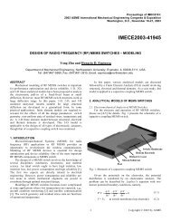
Fig. 1 Diagrams depicting the different ways in which the average
velocity can be estimated: „a… average velocity method,
„b… average image method, „c… average correlation method
averaging of the image fields can create too many particle images
in the interrogation spot and reduce the visibility of individual
particle images.
The 2-D spatial correlation function of the average of A and B
image fields is defined as
R AB sĀXB¯Xsd 2 X, (3)
where Ā1/N N
i1 A i is the average operator, averaging over N
realizations of the flow field. Expanding the integrand of 3
yields
R AB s
A 1 B 1 A 1 B 2 A 1 B 3 ¯A 1 B N
A 2 B 1 A 2 B 2 A 2 B 3 ¯A 2 B N
A 3 B 1 A 3 B 2 A 3 B 3 ¯A 3 B N
" " " d 2 X.
" " "
" " "
A N B 1 A N B 2 A N B 3 ¯A N B N
Following the discussion in the previous section, if A and B
represent paired single-exposure image fields separated by a
known time interval, t, which are cross correlated, and if the
mean image intensity is subtracted before correlation, then all N
N terms in 4 are contained in the R D component of R.
Only the N diagonal terms in 4 contribute to signal. The
N(N1) off diagonal terms represent random particle correlation
(4)
286 Õ Vol. 122, JUNE 2000 Transactions of the ASME

across different realizations, which produce noise in the correlation
function that can reduce the accuracy of the measurement and
cause erroneous measurements. Since the off diagonal terms are
random and uniformly distributed throughout the correlation
plane, they may or may not contaminate the signal peak. The
number of noise terms increases as N 2 , while the number of signal
terms increases as N.
In demanding situations when particle-number density is low,
or when small interrogation regions are chosen to produce high
spatial resolution, it may be impossible to obtain an adequate
signal from instantaneous cross correlation analysis. Clearly, averaging
the particle-image fields over several realizations and then
correlating can increase the signal-to-noise ratio. However, if the
number of realizations used in the average is beyond an optimal
number, the signal-to-noise ratio can be reduced by further increases
in N. Loss of signal occurs because the number of nondiagonal
noise terms increases faster than the diagonal signal
terms. The optimal number of realizations depends upon many
factors including, interrogation spot size, particle-image number
density, and particle-image quality.
3.3 Average Correlation Method. A third method for estimating
average displacement fields is to calculate instantaneous
correlation functions, average the correlation function, and then
determine the location of the signal peak location. The Average
Correlation Method, is shown graphically in Fig. 1c. The average
of instantaneous correlation functions over N realizations can
be written as
R¯AB sAXBXsd 2 XAXBXsd 2 X.
(5)
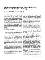
Figure 2 shows several instantaneous correlation functions, and
an average correlation function calculated by averaging 20 instantaneous
correlation functions. The instantaneous correlation functions
are characteristic of micro-PIV data and were obtained from
an actual micro-PIV experiment. The instantaneous correlation
functions contain significant amounts of noise that can lead to
inaccurate or unreliable measurements. This noise is substantially
less in the average correlation function.
Since the operations of averaging and integration commute, the
average operator can be taken inside of the integral so that
R¯AB sA 1 B 1 A 2 B 2 A 3 B 3 ¯A N B N d 2 X. (6)
Fig. 2 Instantaneous cross correlation functions that are averaged
together to produce an average correlation function.
The average correlation function has a much higher signal-tonoise
ratio than the instantaneous correlation functions.
From 6, the average correlation function contains only the
diagonal i.e., signal terms of 4. Therefore, this type of average
produces a much higher signal-to-noise ratio than the alternative
methods that have been discussed previously. The number of signal
terms increases linearly with the number of realizations, N.
Unlike the average image method, there is no penalty for including
large numbers of realizations in the average. Since the average
operator is applied to the correlation function before peak detection,
the probability of erroneous measurements is greatly
reduced.
4 Application to Microchannel Flow
The three different averaging algorithms were applied to a series
of particle image fields taken of steady Stokes’ water flow
through a 30 m300 m glass microchannel. Details of the
same experiment but for a different flow rate are discussed by
Meinhart et al. 10. The out of plane measurement resolution is
related to the depth of field of the microscope optics, and is estimated
to be approximately 1.8 m. Based on the discussion of
Santiago et al. 9, the error due to Brownian motion for a single
particle is estimated to be less than 3 percent full-scale error. The
interrogation spot size was 1664 pixels and 2472 pixels, for
window 1 and window 2, respectively. The relative offset between
the windows was adjusted adaptively to approximate the particle
image displacement at each measurement location. The interrogation
windows were chosen to be small and have a high aspect ratio
to achieve high spatial resolution in the wall-normal direction.
The signal-to-noise ratio from standard correlation techniques
was relatively low, because there was an average of only 2.5
particle images located in each 1664 pixel interrogation window.
The signal-to-noise ratio could be improved by increasing
the size of the correlation windows, but with reduced spatial resolution.
Alternatively, the particle concentration in the flow field
could be increased, but that would increase the number of out of
focus particles, and produce more background image noise.
Figure 3a shows an instantaneous velocity-vector field, calculated
using a standard cross correlation technique without any
type of vector validation or smoothing applied to the field. The
velocity measurements contained in the row closest to the wall are
not considered to be accurate, because part of their interrogation
region lies outside the flow domain. The velocity measurements
are noisy, and approximately 20 percent appear to be erroneous.
An average over 20 instantaneous velocity fields is shown in Fig.
3b. Averaging reduces small random noise in the instantaneous
fields. However, the large errors associated with the erroneous
measurements are not averaged out quickly. The application of
vector validation algorithms can usually eliminate errors due to
erroneous measurements producing accurate velocity measurements,
however a priori knowledge of the flow field is required.
The same series of double-frame particle image fields were correlated,
the correlation functions were averaged, and then the locations
of the signal peaks in the correlation plane were determined,
following the average correlation method depicted in Fig.
1c. The resulting velocity-vector field is shown in Fig. 3c. No
vector validation or smoothing has been applied to this field. The
field contains only 0.5–1 percent erroneous measurements and has
less noise than the vector fields shown in Figs. 3a and 3b.
The relative performance of the three averaging algorithms was
quantitatively compared by varying the number of realizations
used in the average, from one to twenty. The fraction of valid
measurements for each average was determined by identifying the
number of velocity measurements in which the streamwise component
of velocity deviated by more than 10 percent from the
known solution at each point. For this comparison, the known
solution was the velocity vector field estimated by applying the
average correlation technique to 20 realizations, and then smoothing
the flow field.
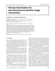
Figure 4 shows the fraction of valid measurements for each of
the three algorithms as a function of the number of realizations
used in the average. The average correlation method better than
performs the other two methods, and produces less than 0.5–1
percent erroneous measurements after averaging eight realizations.
The average image method produces about 95 percent reliable
velocity measurements, and reaches a maximum at four averages.
Further increases in the number of realizations used to
Journal of Fluids Engineering JUNE 2000, Vol. 122 Õ 287

Fig. 4 Comparison of the performance of the three averaging
techniques: average velocity , average image , and average
correlation
Conclusions
Three PIV algorithms are compared for estimated timeaveraged
velocity fields. The process of obtaining PIV measurements
involves three primary steps: 1 particle image acquisition,
2 particle image correlation, and 3 correlation peak detection.
In order to obtain average velocity fields, an averaging operator
must be applied to the data. When signal strength is sufficient, the
average can be applied after steps 1, 2, or 3. However, in demanding
situations when signal strength is weak, the order in which the
average operator is applied is important. The correlation and peak
detection operators are nonlinear and do not commute with the
average operator. Optimal signal strength can be achieved by first
calculating instantaneous correlation functions, and then averaging
the correlation functions before locating the signal peak.
The theoretical observations were confirmed by applying the
three different algorithms to experimental particle image data
from a 30 m300 m microchannel flow. The results showed
that, by averaging instantaneous correlation functions before signal
peak detection, high quality velocity data can be obtained with
less than 0.5–1 percent erroneous measurements, even when only
an average of 2.5 particle images were contained in a single interrogation
spot.
Acknowledgments
This research is supported by AFOSR/DARPA F49620-97-1-
0515, DARPA F33615-98-1-2853, and JPL/NASA 961270.
Fig. 3 Velocity vector fields showing the results from the different
methods of calculation: „a… instantaneous velocity field,
„b… time average of twenty instantaneous velocity fields, „c… velocity
field calculated from time-averaged correlation functions
average the images decreases the signal to noise of the average
particle-image field, and produces noise in the correlation plane
due to random correlation between nonpaired particle images. The
average velocity method reaches a maximum of 88 percent reliable
measurements using two velocity averages. Further increases
in the number of averages decreases the number of reliable measurements,
due to an increase in the probability of an encountering
an erroneous measurement.
References
1 Adrian, R. J., and Yao, C. S., 1985, ‘‘Pulsed laser technique application to
liquid and gaseous flows and the scattering power of seed materials,’’ Appl.
Opt., 24, No. 1, pp. 44–52.
2 Adrian, R. J., 1988, ‘‘Double Exposure, Multiple-field particle image velocimetry
for turbulent probability density,’’ Opt. Lasers Eng., 9, pp. 211–228.
3 Adrian, R. J., 1991, ‘‘Particle-imaging techniques for experimental fluid mechanics,’’
Annu. Rev. Fluid Mech., 23, pp. 261–304.
4 Keane, R. D., and Adrian, R. J., 1991, ‘‘Optimization of particle image velocimeters.
II. Multiple pulsed systems,’’ Meas. Sci. Technol., 2, No. 10, Oct.,
pp. 963–974.
5 Keane, R. D., and Adrian, R. J., 1992, ‘‘Theory of cross-correlation analysis of
PIV images,’’ Appl. Sci. Res., 49, pp. 191–215.
6 Westerweel, J., 1997, ‘‘Fundamentals of digital particle image velocimetry,’’
Meas. Sci. Technol., 8, pp. 1379–1392.
7 Westerweel, J., Draad, A. A., van der Hoeven, J. G. Th., and van Oord, J.,
1996, ‘‘Measurement of fully developed turbulent pipe flow with digital PIV,’’
Exp. Fluids, 20, pp. 165–177.
8 Meinhart, C. D., and Adrian, R. J., 1995, ‘‘On the existence of uniform momentum
zones in a turbulent boundary layer,’’ Phys. Fluids, 7, No. 4, pp.
694–696.
9 Santiago, J. G., Wereley, S. T., Meinhart, C. D., Beebe, D. J., and Adrian, R.
288 Õ Vol. 122, JUNE 2000 Transactions of the ASME

J., 1998, ‘‘A micro particle image velocimetry system,’’ Exp. Fluids, 25, No.
4, pp. 316–319.
10 Meinhart, C. D., Wereley, S. T., and Santiago, J. G., ‘‘PIV measurements of a
microchannel flow,’’ Exp. Fluids, 27, pp. 414–419.
11 Tieu, A. K., Mackenzie, M. R., and Li, E. B., 1995, ‘‘Measurements in microscopic
flow with a solid-state LDA,’’ Exp. Fluids, 19, pp. 293–294.
12 Meinhart, C. D., Barnhart, D. H., and Adrian, R. J., 1994, ‘‘Interrogation and
validation of three-dimensional vector fields,’’ Developments in Laser Techniques
and Applications to Fluid Mechanics, R. J. Adrian et al., eds.,
Springer-Verlag, Berlin, pp. 379–391.
13 Westerweel, J., 1993, ‘‘Efficient detection of spurious vectors in particle image
velocimetry data,’’ Exp. Fluids, 16, pp. 236–247.
Journal of Fluids Engineering JUNE 2000, Vol. 122 Õ 289