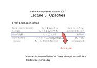
lecture notes

Introduction to Numerical
Hydrodynamics and Radiative Transfer
Part II: Hydrodynamics, Lecture 5
HT 2009
Susanne Höfner
Susanne.Hoefner@fysast.uu.se

Introduction to Numerical Hydrodynamics
2. The Linear Advection Equation
2.6 PLM and Non-linear Schemes

Linear Advection – The Story So Far ...
first order schemes:
modified equation: advection-diffusion equation
∂
∂t
u ∂
∂ x = D ∂2
∂ x 2
→ diffusive behaviour of the numerical solution

Linear Advection – The Story So Far ...
second order schemes:
modified equation: dispersive equation
∂
∂t
u ∂
∂ x = ∂3
∂ x 3
→ oscillating behaviour of the numerical solution
waves:
group velocity
c g = u + 3µ k2
µ < 0 µ > 0
c g < u
c g > u

Numerical Schemes ... Alternatives
Question:
How to construct a numerical scheme for advection which is more
accurate than a first-order scheme (less diffusion, sharper
gradients), but which doesn't develop oscillations like the second
order schemes which we have investigated so far
Let's start with recalling a few important concepts ...

Integral Form and Flux Centering
Any solution of the advection equation in differential form
involves derivatives.
However, any function – even a discontinuous one – can be
propagated along characteristics (see, e.g., Homework 1).
In certain cases, it may be important to avoid derivatives and/or
discontinuities.
Transformation: linear advection equation in integral form:
Figure courtesy of Bernd Freytag
... for one grid cell and one time step:

Update Formula in Conservation Form
After computing the fluxes at the cell boundaries
that characterize a method
(e.g. from the fluxes in the cells: )
the update can be done by the formula
This is the conservation form because the density changes only
due to fluxes through the boundaries, and is conserved otherwise:

Update Formula in Conservation Form
After computing the fluxes at the cell boundaries
that characterize a method
(e.g. from the fluxes in the cells: )
the update can be done by the formula
This is the conservation form because the density changes only
due to fluxes through the boundaries, and is conserved otherwise.
Guidelines for improved advection:
- keep conservation form
- define more accurate fluxes (reduce diffusion or oscillations)

Improving Advection – RSA Algorithm
Reconstruct – Solve – Average (RSA):
Godunov-type finite-volume scheme
1. Reconstruct ρ(x) from the discrete values ρ i
n (cell averages)
2. Solve the exact problem for ∆t
3. Average this function over each grid cell to obtain ρ i
n+1
Steps 2 and 3 are well-behaved (e.g., conservative) by default,
step 1 is potentially a problem.
Piecewise constant reconstruction (constant value in cell)
→ Godunov's method

Improving Advection – PLM Schemes
The dispersive equation
with
∂
∂t
u ∂
∂ x = ∂3
∂ x 3
0
for
∣ u t
x ∣ 1 c g
u
(Lax-Wendroff)
or
0
for
∣ u t
x ∣ 1 c g
u
(Beam-Warming)
original PDE (linear advection equation):
- constant amplitude (no growth or decay)
- no dispersion (all waves travel at same speed)

PLM Schemes – Examples of Slopes
The dispersive equation
with
∂
∂t
u ∂
∂ x = ∂3
∂ x 3
0
for
∣ u t
x ∣ 1 c g
u
(Lax-Wendroff)
or
0
for
∣ u t
x ∣ 1 c g
u
(Beam-Warming)
original PDE (linear advection equation):
- constant amplitude (no growth or decay)
- no dispersion (all waves travel at same speed)

PLM Schemes – Examples of Slopes
Example: Lax-Wendroff ... the RSA perspective
... applied to piecewise constant data •
• • •
• • •
advection
u∆t = ∆x/2
→
• •
•
•
• •
reconstruction
new cell averages
→ too steep slope causes oscillations ...

PLM Schemes – Examples of Slopes
Example: Lax-Wendroff ... the RSA perspective
... applied to piecewise constant data •
• • •
• • •
advection
u∆t = ∆x/2
→
• •
•
•
• •
reconstruction
new cell averages
→ too steep slope causes oscillations ...

PLM Schemes – Examples of Slopes
Example: Lax-Wendroff ... the RSA perspective
... applied to piecewise constant data •
• • •
• • •
advection
u∆t = ∆x/2
→
• •
•
•
• •
reconstruction
new cell averages
→ too steep slope causes oscillations ...

PLM Schemes – Examples of Slopes
Example: Lax-Wendroff ... the RSA perspective
... applied to piecewise constant data •
• • •
• • •
advection
u∆t = ∆x/2
→
reconstruction
new cell averages
→ too steep slope causes oscillations ...

PLM Schemes – Examples of Slopes
Example: Lax-Wendroff ... the RSA perspective
... applied to piecewise constant data •
• • •
• • •
advection
u∆t = ∆x/2
→
• •
•
•
• •
reconstruction
new cell averages
→ too steep slope causes oscillations ...

PLM Schemes – Examples of Slopes
Example: Lax-Wendroff ... the RSA perspective
... applied to piecewise constant data •
• • •
• • •
advection
u∆t = ∆x/2
→
• •
•
•
• •
reconstruction
new cell averages
→ too steep slope causes oscillations ...

Improving Advection – Monotonicity
The dispersive equation
with
∂
∂t
u ∂
∂ x = ∂3
∂ x 3
0
for
∣ u t
x ∣ 1 c g
u
(Lax-Wendroff)
or
0
for
∣ u t
x ∣ 1 c g
u
(Beam-Warming)
original PDE (linear advection equation):
- constant amplitude (no growth or decay)
- no dispersion (all waves travel at same speed)

PLM Schemes – Slope-Limiter
The dispersive equation
with
∂
∂t
u ∂
∂ x = ∂3
∂ x 3
0
for
∣ u t
x ∣ 1 c g
u
(Lax-Wendroff)
or
for
(Beam-Warming)
original PDE (linear advection equation):
- constant amplitude (no growth or decay)
- no dispersion (all waves travel at same speed)

PLM Scheme with Minmod Slope-Limiter
∂ y
∂t
= D ∂2 y
∂ x 2
Figures courtesy of Bernd Freytag
Stencil diagram and test result (initial condition: red, solution:
blue) for PLM scheme with minmod slope-limiter

PLM Scheme with van Leer Slope-Limiter
∂ y
∂t
= D ∂2 y
∂ x 2
Figures courtesy of Bernd Freytag
Stencil diagram and test result (initial condition: red, solution:
blue) for PLM scheme with van Leer slope-limiter (harmonic
mean of slopes)

PLM Scheme with Superbee Slope-Limiter
∂ y
∂t
= D ∂2 y
∂ x 2
Figures courtesy of Bernd Freytag
Stencil diagram and test result (initial condition: red, solution:
blue) for PLM scheme with Superbee slope-limiter

PPM Scheme
∂ y
∂t
= D ∂2 y
∂ x 2
Figures courtesy of Bernd Freytag
Stencil diagram and test result (initial condition: red, solution:
blue) for PPM scheme with piecewise parabolic reconstruction
(Colella & Woodward, 1984)

WENO Scheme
∂ y
∂t
= D ∂2 y
∂ x 2
Figures courtesy of Bernd Freytag
Stencil diagram and test result (initial condition: red, solution:
blue) for WENO scheme with weighted essentially non-oscillatory
reconstruction (6 th order polynomials, without any Runge-Kutta
sub-steps), see, e.g., Jiang & Shu (1996)