Turbulent Flow and Heat Transfer in a Mixing Elbow

Turbulent Flow and Heat Transfer in a Mixing Elbow
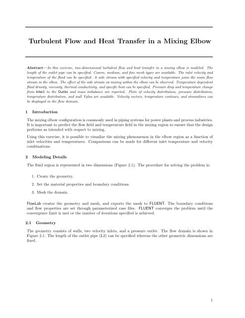
Abstract—In this exercise, two-dimensional turbulent flow and heat transfer in a mixing elbow is modeled. The
length of the outlet pipe can be specified. Coarse, medium, and fine mesh types are available. The inlet velocity and
temperature of the fluid can be specified. A side stream with specified velocity and temperature joins the main flow
stream in the elbow. The effect of the side stream on mixing within the elbow can be observed. Temperature dependent
fluid density, viscosity, thermal conductivity, and specific heat can be specified. Pressure drop and temperature change
from Inlet1 to the Outlet and mass imbalance are reported. Plots of velocity distribution, pressure distribution,
temperature distribution, and wall Yplus are available. Velocity vectors, temperature contours, and streamlines can
be displayed in the flow domain.
1 Introduction
The mixing elbow configuration is commonly used in piping systems for power plants and process industries.
It is important to predict the flow field and temperature field in the mixing region to ensure that the design
performs as intended with respect to mixing.
Using this exercise, it is possible to visualize the mixing phenomenon in the elbow region as a function of
inlet velocities and temperatures. Comparisons can be made for different inlet temperature and velocity
combinations.
2 Modeling Details
The fluid region is represented in two dimensions (Figure 2.1). The procedure for solving the problem is:
1. Create the geometry.
2. Set the material properties and boundary conditions.
3. Mesh the domain.
FlowLab creates the geometry and mesh, and exports the mesh to FLUENT. The boundary conditions
and flow properties are set through parameterized case files. FLUENT converges the problem until the
convergence limit is met or the number of iterations specified is achieved.
2.1 Geometry
The geometry consists of walls, two velocity inlets, and a pressure outlet. The flow domain is shown in
Figure 2.1. The length of the outlet pipe (L2) can be specified whereas the other geometric dimensions are
fixed.
1

2.2 Mesh
Figure 2.1: Geometry
Coarse, medium, and fine mesh types are available. Mesh density varies based upon the assigned Refinement
Factor. The Refinement Factor values for the mesh densities are given in Table 2.1.
Mesh Density Refinement Factor
Fine 1
Medium 1.414
Coarse 2
Table 2.1: Refinement Factor
Using the Refinement Factor, First Cell Height is calculated with the following formula:
F irst Cell Height = Refinement F actor
� Y plus × (Characteristic Length 0.125 × V iscosity 0.875 )
(0.199 × V elocity 0.875 × Density 0.875 )
2 c○ Fluent Inc. [FlowLab 1.2], April 12, 2007
�
(2-1)

Reynolds number is used to determine Yplus. The Yplus values for turbulent flow conditions are summarized
in Table 2.2.
Reynolds Number Flow Regime Yplus/First Cell Height
Re > 20000 Turbulent, Standard Wall Functions Yplus > 30
Table 2.2: Flow Regime Vs. Reynolds Number
The number of intervals along each edge is determined using geometric progression as follows:
⎡
Intervals = INT ⎣ Log
� Edge length×(Growth ratio−1)
F irst Cell Height
Log(Growth ratio)
�⎤
+ 1.0
⎦ (2-2)
The edges are meshed using the First Cell Height and the calculated number of intervals. The entire domain
is meshed using a map scheme. The resulting mesh is shown in Figure 2.2.
2.3 Physical Models for FLUENT
Figure 2.2: Mesh Generated by FlowLab
Based on the Reynolds number, the following physical models are recommended:
Re Model Used
Re > 20000 k − ɛ model
Table 2.3: Turbulence Models Based on Pipe Reynolds Number
Note: The turbulent flow conditions are specified even if the exercise is run using a Reynolds number less
than 20000.
c○ Fluent Inc. [FlowLab 1.2], April 12, 2007 3

2.4 Material Properties
The default properties provided in this exercise represent water. Temperature dependence for material
properties, including density, viscosity, specific heat, and thermal conductivity can be specified through the
following second order polynomial equation:
Property = A0 + (A1 × T) + (A2 × T 2 )
where, A0, A1, and A2 are fluid dependent constants.
Two materials (air and water) are readily available in the exercise. A user-specified option is available for
defining any additional material. The default values for the constants provided in the exercise are listed in
Table 2.4. All the properties in the table are in SI units.
A0 A1 A2
Air
Density 1.6762173930448108 -2.1923479098913349e-03 8.1439756283488314e-07
Viscosity 7.0587110995982522e-06 4.1957623160204437e-08 -6.3559854911267468e-12
Specific Heat (Cp) 9.4235900447551762e+02 1.9317284714300231e-01 -9.0424058617075095e-07
Thermal Conductivity (K) 1.2342068184925949e-02 5.1944011288572976e-05 3.5801428546445151e-09
Water
Density 8.9696916169663916e+02 1.0033551606212396 -2.2382670604180386e-03
Viscosity 1.2788719593450531e-02 -6.5107718802936428e-05 8.4504799548279901e-08
Specific Heat (Cp) 4.9535071710897391e+03 -5.0376115189154564 8.1953698475433333e-03
Thermal Conductivity (K) -4.8376708074539942e-01 5.8597967250142054e-03 -7.3404856013554481e-06
2.5 Boundary Conditions
Table 2.4: Polynomial Constants for Air and Water
The following boundary conditions can be specified at both the inlets:
• Inlet fluid velocity
• Inlet fluid temperature
• Wall Roughness
The following boundary conditions are assigned in FLUENT:
Boundary Assigned as
Inlet 1 Velocity inlet
Inlet 2 Velocity inlet
Outlet Pressure outlet
All the walls including Wall 3 Wall
Table 2.5: Boundary Conditions Assigned in FLUENT
4 c○ Fluent Inc. [FlowLab 1.2], April 12, 2007

2.6 Solution
The Reynolds number at both inlets is calculated based on the specified boundary conditions and material
properties.
The mesh is exported to FLUENT along with the physical properties and the initial conditions specified.
The material properties and the initial conditions are read through the case file. Instructions for the solver
are provided through a journal file. When the solution is converged or the specified number of iterations
is met, FLUENT exports data to a neutral file and to .xy plot files. GAMBIT reads the neutral file for
postprocessing.
3 Scope and Limitations
This exercise is designed to compute turbulent flow and heat transfer in a mixing junction for Reynolds
numbers greater than 20000. The k − ɛ turbulence model will be applied even if boundary conditions are
specified such that Reynolds number is less than 20000. It is recommended to use this exercise only to
simulate flows where Reynolds number is greater than 20000 at both inlets.
Difficulty in obtaining convergence or poor accuracy may result if input values are used outside the upper
and lower limits suggested in the problem overview.
4 Exercise Results
4.1 Reports
The following reports are available:
• Total pressure drop from Inlet1 to Outlet.
• Temperature change from Inlet1 to Outlet.
• Mass imbalance
4.2 XY Plots
The plots reported by FlowLab include:
• Residuals
• Velocity distribution at Outlet.
• Static pressure distribution at Wall3
• Temperature distribution at Outlet.
• Wall Yplus distribution.
Figures 4.1 and 4.2 show velocity distribution and temperature distribution respectively at the outlet section
(Outlet).
c○ Fluent Inc. [FlowLab 1.2], April 12, 2007 5

Figure 4.1: Velocity Distribution at Outlet
Figure 4.2: Temperature Distribution at Outlet
6 c○ Fluent Inc. [FlowLab 1.2], April 12, 2007

4.3 Contour Plots
Contour plots of pressure, temperature, velocity, and stream function are available. Velocity vector plots
can also be displayed.
5 Comparative Study
Figure 4.3: Contours of Static Temperature
Figure 5.1 shows temperature distribution at the outlet section for various Inlet2 velocities. Temperature
gradient at the outlet is shown to be dependent upon Inlet2 velocity.
Figure 5.1: Temperature Distribution at Outlet for Different Inlet2 Velocities
c○ Fluent Inc. [FlowLab 1.2], April 12, 2007 7

6 Reference
[1] Incropera F. P. and DeWitt David P., “Fundamentals of Heat and Mass Transfer”, John Wiley and
Sons, Fourth Edition.
8 c○ Fluent Inc. [FlowLab 1.2], April 12, 2007