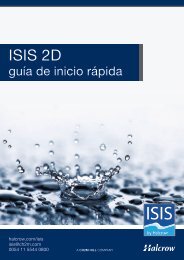
ISIS 2D Quick Start Guide - Halcrow

Cost effective, integrated modelling solutions
Think saving, think ISIS, think Halcrow
ISIS 2D
quick start guide
0845 094 7994
halcrow.com/isis
isis@halcrow.com
A CH2M HILL COMPANY
by Halcrow
TECHNOLOGY
Technology

Table of Contents
ISIS 2D Quick Start Guide..................................................................................................... 2
Overview ......................................................................................................................... 2
Overview ......................................................................................................................... 2
Starting ISIS 2D and Basic Concepts .................................................................................... 2
Starting ISIS 2D............................................................................................................. 2
Principles of Working with ISIS 2D .................................................................................... 3
Basic Concepts............................................................................................................... 3
Files ............................................................................................................................. 4
Example files ................................................................................................................. 4
How to Run an ISIS 2D Model ............................................................................................. 5
Introduction .................................................................................................................. 5
Description of the steps for setting up a single domain ISIS 2D model..................................... 5
Example data................................................................................................................. 6
Preparation of the GIS data (steps 1-5).............................................................................. 6
Preparation of the data for the boundary and initial conditions and roughness (steps 6 - 7)......... 7
Setting up the run parameters for your simulation (step 8).................................................... 9
Setting up the parameters for the results output (step 9)...................................................... 9
Running the ISIS 2D Simulation...................................................................................... 10
Viewing the Results Files of the ISIS 2D Simulation............................................................ 10
How to Run an ISIS 2D 1D - 2D Linked Model ...................................................................... 13
Running an existing ISIS 1D-2D model using the ISIS 2D Interface Tool................................ 13
Viewing ISIS 2D Model Results ....................................................................................... 15
How to Build a New ISIS 2D Model..................................................................................... 15
How to View the ISIS 2D Results Files ................................................................................ 29
1. Viewing the Mass Balance File ..................................................................................... 29
2. Viewing a time series plot at a particular point............................................................... 31
3. Viewing a Cross-section Plot using ISIS Mapper ............................................................. 35
4. Animation of the 2D Model Results in ISIS Mapper.......................................................... 37
5. Generation of a Flood Extents Map in ISIS Mapper.......................................................... 38
1

ISIS 2D Quick Start Guide
ISIS 2D Quick Start Guide
Overview
This quick start guide enables first time users to understand how to use ISIS 2D, to construct and run
simple 2D and linked ISIS 1D-2D models and how to view ISIS 2D model results. The guide also
explains some of the basic concepts of ISIS 2D model construction and the various files used to run a
model.
• Chapter Starting ISIS 2D and Basic Concepts explains how to start using your ISIS
2D software and goes through some basic concepts.
• Chapter How to Run an ISIS 2D Model illustrates the principles of building and
running an ISIS 2D model and explains principles about viewing the obtained
results using ISIS Mapper.
• Chapter How to Run an ISIS 2D 1D - 2D Linked Model shows an example of
running an already prepared linked model.
• Chapter How to Build a New ISIS 2D Model shows an example of creating the files
that define a new ISIS 2D model starting from a DEM and using tools provided in
ISIS Mapper
• Chapter How to View the ISIS 2D Results Files describes the steps needed for the
visualisation of the results of the ISIS 2D simulation.
Overview
This quick start guide enables first time users to understand how to use ISIS 2D, to construct and run
simple 2D and linked ISIS 1D-2D models and how to view ISIS 2D model results. The guide also
explains some of the basic concepts of ISIS 2D model construction and the various files used to run a
model.
• Chapter Starting ISIS 2D and Basic Concepts explains how to start using your ISIS
2D software and goes through some basic concepts.
• Chapter How to Run an ISIS 2D Model illustrates the principles of building and
running an ISIS 2D model and explains principles about viewing the obtained
results using ISIS Mapper.
• Chapter How to Run an ISIS 2D 1D - 2D Linked Model shows an example of
running an already prepared linked model.
• Chapter How to Build a New ISIS 2D Model shows an example of creating the files
that define a new ISIS 2D model starting from a DEM and using tools provided in
ISIS Mapper
• Chapter How to View the ISIS 2D Results Files describes the steps needed for the
visualisation of the results of the ISIS 2D simulation.
Starting ISIS 2D and Basic Concepts
Starting ISIS 2D
Once you have installed the ISIS software, you are ready to use ISIS 2D. To open the ISIS 2D
Interface please go to the Start menu, select Programs, then select the ISIS group and click on the
ISIS 2D item. Alternatively you can click on ISIS icon and then open the ISIS 2D Interface from
the Run menu, the menu item ISIS 2D. Please note that you can also open ISIS 2D Interface Tool by
clicking on the button on the toolbar of the Network Properties window of ISIS. If you have any
questions please do not hesitate to contact ISIS support (details are at the foot of this page).
2

ISIS 2D Quick Start Guide
Principles of Working with ISIS 2D
There are several phases when working with ISIS 2D models and various parts of the ISIS 2D
software are used during the process.
The main phases of working with the 2D models are:
1. Pre-processing of the input files for running ISIS 2D simulation;
2. Preparation of the ISIS 2D control XML file;
3. Running the ISIS 2D simulation;
4. Viewing ISIS 2D results files;
ISIS Mapper can be used for pre-processing of the input files for running the ISIS 2D simulation and
for viewing ISIS 2D results files; ISIS Mapper can be accessed by clicking the ISIS Mapper icon or
selecting > Tools > ISIS Mapper in ISIS Network Properties window of ISIS. ISIS Mapper is a GIS
tool specially designed for doing the pre & post processing of ISIS 1D, ISIS 2D and TUFLOW 2D
models.
Other GIS software can also be used to generate input files for ISIS 2D.
There are two ways of running the calculations using ISIS 2D models: using the command prompt or
the ISIS 2D Interface Tool.
ISIS 2D Interface Tool can be accessed by selecting > Run > ISIS 2D in the ISIS Network Properties
window. This option is described in more details in ISIS 2D Manual. The ISIS 2D Interface is a special
application designed for making the creation of ISIS 2D XML control files easier for the users.
Preparation of the ISIS 2D control XML file is done by using both ISIS Mapper and the ISIS 2D
Interface. More details about this can be found in ISIS 2D Manual.
Basic Concepts
ISIS 2D is a shallow water flow model which predicts depths and velocities on a regular square grid,
and can link to an ISIS 1D model representing flows in a channel. It has been designed to model flows
in coastal, estuary and floodplain environments. At the core of ISIS 2D, there are two numerical
schemes that are specifically developed to tackle different types of hydraulic conditions: ADI
(Alternating Direction Implicit) and TVD (Total Variation Diminishing).
The main differences between these two themes are listed in the Table 1 below:
Modelling rapidly varying
flows
ADI
May not represent higher Froude
number flows correctly
TVD
Accurate representation
of high Froude number
flows, shocks and jumps
Computation Times Short run times Longer run times
Time steps Long time steps possible Shorter time steps
needed for model to run
Stability
Mass Conservation
Some instabilities/oscillations in the
solution may become apparent for
simulations with Froude numbers
approaching or exceeding one, or
too large a time step
Generates acceptable mass balance
errors for well set up 2D and linked
1D-2D models
Generates more stable
and smoother solutions
Can lead to larger (but
still acceptable) mass
balance errors for linked
1D-2D models
3

ISIS 2D Quick Start Guide
Table 1. Differences between the ADI and the TVD schemes used in ISIS 2D.
In order to run an ISIS 2D model the following information is needed:
4
• A geographic model domain extent: to represent an extent of the possible
flooding;
• Topography (ground level data and information of the locations of defences) of
the area under consideration;
• Hydrological data in the form of the boundary and initial conditions: to represent
the flows entering and leaving the model extent and the water levels passed to
the model as well as the initial state of the system;
• Roughness coefficients: to describe variation of roughness coefficients in different
parts of the model (can be represented by one value for all the domain extent);
• Such data as duration of a simulation period, time step, grid cell size etc: to
represent various run parameters of the model;
ISIS 2D uses an XML (Extensible Markup Language) control file to describe the model composition.
The locations of the model input and output files and various parameters are described by an XML
control file. This control file provides all the necessary information for running ISIS 2D numerical
engine.
As mentioned earlier, the ISIS 2D Interface Tool helps the user build 2D models and do the pre & post
processing work. ISIS Mapper, a GIS tool specially designed for doing the pre & post processing of
ISIS 1D, ISIS 2D and TUFLOW 2D models, is supplied together with ISIS 2D Interface Tool as part of
ISIS 2D product.
Setting up an ISIS 2D model effectively means completing a valid ISIS 2D XML control file (validate
against the predefined XML schema) and preparing the associated data files.
Files
ISIS uses a range of different files to manage model data and results. The data formats that ISIS 2D
uses are:
XML file (.xml file): this is the format in which ISIS 2D control file is written;
Comma Separated Values format (.csv file): The mass balance ISIS 2D output files, and depth,
elevation, flow or velocity at user specified points in the domain are saved in this format;
ESRI ASCII raster grid file (.asc file): model domain extents, topography, boundary & initial
conditions, roughness coefficients can be represented by an ASCII grid.
ESRI shapefile (point, polyline, and polygon) (.shp file): active computation area, boundary & initial
conditions and topography, link lines are represented by shapefiles.
2D Model Results Data file (.dat file, .2dm and .sup files): ISIS 2D model results are written in such a
format that enables them to be viewed, visualised and analysed by ISIS Mapper. The files with the
extension .dat contain all the results of ISIS 2D simulation, the files with the extension .2dm contain
the geographic information about the 2D mesh. The .sup file, which contains a list of the .2dm and
.dat files associated with the model results, is provided for compatibility with other software which
reads this file format.
Standard text file: the boundary condition file for ISIS 1D simulation (.ied file), ISIS 2D log file are
saved in this format (normally .log or as specified by the user in the ISIS 2D Control XML file) and
ISIS 1D event file (.ief file). The last file contains the information regarding the parameters and input
and results file for ISIS 1D simulation.
Example files
The "isis" folder of your machine (upon the installation of ISIS) should already contain some example
files. Some of them will be used in this Chapter. The default location for your ISIS data is C:\isis\data
(if ISIS is installed at a location other than the default folder, it will be xxx\xxx\isis\data where xxx
stands for where ISIS is installed). The ISIS 2D related examples are placed into ISIS 2D subfolder
(eg C:\isis\data\examples\ISIS 2D). Some of these files are used when describing various operations
in this Quick Start Guide.

ISIS 2D Quick Start Guide
Digital Terrain Models (DTMs) and digital aerial photography for the ISIS 2D example data have been
kindly supplied by Bluesky. These data are provided for demonstration purposes only, and should not
be used for commercial or fee earning work. For further details and acknowledgements, please see the
file Sample Data ReadMe.doc, installed with the examples data, or visit www.bluesky-world.com.
How to Run an ISIS 2D Model
Introduction
This Chapter illustrates the process of setting up a single domain ISIS 2D model.
Building of the ISIS 2D model can be divided into two actions:
• Preparation of the model data;
• Creation of the ISIS 2D control XML file.
ISIS 2D control XML file is a project file that tells the ISIS 2D software where all the input files are,
what the run parameters are and where the output files should be placed. There are certain tags
allocated for each piece of information the file contains.
ISIS 2D control XML file can be created using ISIS Mapper and ISIS 2D User Interface.
This Chapter explains which the input files for the ISIS 2D simulation are and the steps needed to run
the prepared file. The example files are located in ISIS 2D\Site 1 folder
(XXXXX\data\examples\ISIS2D\Site 1 where XXXXX stands for the folder where ISIS has been
installed i.e. c:\isis). Please note the ISIS 2D control XML file is already prepared for the model as well
as the other input files, so there is no need for the users to draw the files themselves, however they
are welcome to open the files in ISIS Mapper as described in the chapter below.
Description of the steps for setting up a single domain ISIS 2D model
ISIS 2D simulation needs geographical information (such as domain model extent, topographical data
etc), hydrological data (boundary and initial conditions and roughness) and run parameters for a
particular model. Preparation of the model data comprises 9 steps (mentioned below). Steps 1-5 are
related to preparation of the GIS files needed for the model and steps 6-9 describe the way how the
hydrological input data and the parameters of the simulation and the results output are set up. The
steps for setting up a single domain ISIS 2D model are:
1. Setting up a ground level data. This data is in a form of an ASCII grid.
2. Setting up a shapefile that represents a computational area. This file should be
an ESRI polygon shape file. This is known as a computational area shapefile. This
file can be created in ISIS Mapper. Alternatively, the user can supply geographic
coordinates for the computational area, or they are derived from the topography
data (see below).
3. Setting up a shapefile that represents an active area (if necessary). This file
should be an ESRI polygon shape file. This is known as an active area shapefile.
This file can be created in ISIS Mapper. This shapefile defines an area within a
computational area which will be used for calculating ISIS 2D model results. If
the file is not setup and not specified in the ISIS 2D control XML file, than the
ISIS 2D model results calculations will be carried out on the computational area.
4. Setting up a shapefile that represents a line with locations for introducing flows
into the 2D system (i.e. boundary conditions). This file should be an ESRI
polyline shapefile. This file is also known as an ISIS 2D model boundary line file.
This line can be created in ISIS Mapper.
5. Setting up a shape file that represents topographic features (defence systems).
This file can be a point, a polyline or a polygon shapefile depending on a shape of
the defence system. This file is also called a topographic feature file. This file can
be created in ISIS Mapper.
6. Setting up the boundary conditions data for the model. The boundary conditions
can be represented by a time series or a fixed value. This information can be
5

ISIS 2D Quick Start Guide
Example data
either mentioned in the ISIS 2D XML file or provided in an ISIS boundary
conditions .ied file, which is referenced in the ISIS 2D XML file.
7. Setting up the data for roughness and for initial conditions for your model. This
information can be either mentioned in the ISIS 2D XML file or provided in an
ISIS boundary conditions .ied file, which is referenced in the ISIS 2D control XML
file.
8. Setting up the run parameters for your simulation (e.g. start time and date, run
time etc). This information should be mentioned in the ISIS 2D control XML file.
9. Setting up the parameters of the results output (e.g. locations and the format of
the result files).
For the purposes of illustration some of these files have already been created and have been placed to
the examples folder: C:\ isis\data\examples\ISIS2D\Site 1\GIS
The ISIS 2D control XML file (DefenceBreach.xml) has also been created and is located in the
folder: C:\ isis\data\examples\ISIS2D\Site 1
If you open the example XML file in the ISIS 2D Interface Tool, you will be able to see most of the
data explained below under certain tabs of the tool. The paragraphs below will explain which tab to
look at in the ISIS 2D User Interface Tool (All the tabs mentioned are located on the Domains tab).
The tool can be opened by going to Start menu, selecting Programs, then selecting the ISIS group
and clicking on the ISIS 2D item. In order to open the file you need to go to menu File and then
Open in the ISIS 2D User Interface Tool and select the file DefenceBreach.xml.
More details about this tool can be found in the Chapter "Preparation of the ISIS 2D Control XML file".
Preparation of the GIS data (steps 1-5)
The Chapter "Preprocessing of the ISIS 2D GIS Input Files" of ISIS 2D Manual and the Chapter How to
Build a New ISIS 2D Model of this Quick Start Guide provide some guidelines on how to use ISIS
Mapper to create the shapefiles mentioned above (Steps 1-5).
The data that you need now comprises the following files:
1. An ASCII raster grid: 5M_DTM.asc (with the ground elevation data for the whole domain);
2. An ESRI polygon shapefile: River_Active_Area.shp (with the information about the active area)
3. An ESRI polyline shapefile: Defence_BC.shp (representing an ISIS 2D model boundary line)
If you load these three files (in the ISIS Mapper user interface, in the Layer Tab of the main toolbar in
the ISIS Mapper Interface select Add Layer. The Figure 1 below shows the files mentioned above
loaded into ISIS Mapper:
6

ISIS 2D Quick Start Guide
Figure 1. ISIS 2D model domain extents and the corresponding ISIS 2D model input files for the
example
described in this Chapter How to Run an ISIS 2D Model
Please note that on the tabs "Grid Data" and "Boundary Conditions" of ISIS 2D Interface Tool you can
see the names of some of the files mentioned at this section of the Chapter. Figure 2 shows the
Boundary Conditions tab of the ISIS 2D Interface Tool (found within the Domains tab) where the
user can see the Defence_BC.shp file mentioned in the field Boundary Filename.
Preparation of the data for the boundary and initial conditions and roughness
(steps 6 - 7)
This Section of the Chapter continues to describe the ways of preparing the input data for the ISIS 2D
simulation.
You need to make sure that you have the boundary conditions for your model. The boundary
condition (BC) shows how much water is entering the domain at a certain time. There are 5 types of
boundary conditions that users can choose from:
1. Total Flow BC (Total flow);
2. Flow per Unit Width BC (Flow per unit width);
3. Vertical Flow BC (Vertical flow)
4. Vertical Flow per Unit Width BC (Vertical flow per unit width)
5. Elevation BC (Elevation).
The BC can be represented by a time series or by a fixed value. The values can be "hard-coded" within
the ISIS 2D project XML file or could be taken from an ISIS boundary conditions .ied file. For this
7

ISIS 2D Quick Start Guide
example, we use the Vertical Flow BC and the values for this BC are shown in a flow hydrograph in the
Table 2 below:
Time (second) 0 900 3600
Flow (m^3/s) 0 100 0
Table 2. Hydrograph used as a boundary condition for the Site 1\DefenceBreach model example
On Figure 2 the user can see the hydrograph used as a boundary condition for this model. If creating
the model from scratch the user can enter the values on this tab of the ISIS 2D Interface tool.
Figure 2. The Boundary Conditions Tab of the ISIS 2D User Interface showing the BC parameters for
the sample simulation
The roughness and the boundary and initial conditions values for ISIS 2D simulation can be set up in
ISIS 2D Interface tool as well, however for the purposes of the Quick Start Guide these values have
already been set up in the ISIS 2D control XML file (DefenceBreach.xml). More information about
using the ISIS 2D Interface for setting up these values can be found in Chapter Preparation of an
ISIS 2D Control XML File Using the ISIS 2D Interface
8

Setting up the run parameters for your simulation (step 8)
ISIS 2D Quick Start Guide
In this example we use ADI scheme as the numerical Scheme for calculations. Regarding the choice
of time step there are some guidelines that take into account the relationship between the space step
(dimension of the grid with ground elevation data) and the time step (dt/dx): these schemes work
best if dt/dx is in the range 1/2 to 1/40 for ADI scheme and 1/10 to 1/100 for TVD scheme. Based on
these recommendations the time step will be set to be equal to 2 s. Please note the value for the
space step (dx) used in this example is 10 m which is shown in the Grid Size field of the Grid Data
tab of the ISIS 2D Interface Tool. The value of 10 m is one of the extent parameters for the
computational area specified when the rectangular extent computational area is drawn.
We will set Run Time (simulation period) for this model to be 1 hour; the initial conditions for this
model are set as water level of 0 m all over the computational area ("globally" if using the terminology
of the XML file). Please note that for cells where the ground is above this water level, zero depth is
used. The roughness will be set as Manning's coefficient n=0.05 in all cells of the computational area
("globally").
Figure 3. The Run Details Tab of the ISIS 2D User Interface showing the run parameters for the
sample simulation
All these parameters except the Manning's coefficient (roughness) can be seen on the tab Run
Details of ISIS 2D User Interface Tool (Domains Tab) as shown on Figure 3. The roughness values
are set up on the Grid Data Tab of the Domains Tab.
Setting up the parameters for the results output (step 9)
9

ISIS 2D Quick Start Guide
The user has the ability to specify such output parameters as locations and names of the result files,
the variables within the data to be contained in the result files (water level, velocity etc). The user can
choose the period between model outputs being saved to disk. A longer period will result in smaller
output files and save disk space. These parameters can be seen on the tab "Model Outputs" of the
ISIS 2D User Interface.
Running the ISIS 2D Simulation
Normally after you have set up the data or made sure that it is all in place, you can start the ISIS 2D
Simulation. As it was mentioned earlier the ISIS 2D control XML file DefenceBreach.xml has already
been prepared and supplied with the ISIS installation. See the Example Files Section of this Chapter
for more details about opening the tool and this particular file. In order to start the ISIS 2D Simulation
in ISIS 2D Interface please go to the menu Run and then select the item ISIS 2D Simulation. After
the simulation has been run you should get a command prompt message saying "Run successful -
stopping. Press return to close".
Now you should be able to see the results in a new folder in C:\isis\data\examples\ISIS 2D\Site 1
(The location will vary if ISIS is installed somewhere else). The next section explains how the user can
view the results of the ISIS 2D Simulation.
Viewing the Results Files of the ISIS 2D Simulation
1) Launch ISIS Mapper and load the ground grid.
In order to view the 2D model results, launch ISIS Mapper and load the ground grid.
ISIS Mapper can be launched from:
• within the main ISIS interface (Network Properties window) by clicking on the
Mapper icon located in the upper right of the main toolbar
• within the ISIS 2D interface by selecting ISIS Mapper from the Run menu
The ground grid for this example is 5M_DTM.asc stored in the Site 1\GIS folder. In the main toolbar of
the ISIS Mapper interface, select Layer Tab and then Add Layer to add a new GIS file to the map
view. When prompted, navigate to the Site 1/GIS folder and select the 5M_DTM.asc grid (see Figure
4).
Figure 4. Loading a ground grid into ISIS Mapper
The image (aerial photo) which you can see on Figures 1 and 7 is Airphoto.jpg, which you can find in
the Site 1\GIS folder. This image file can be loaded into ISIS Mapper in the same manner as the
ground grid data.
For more details on how to load a grid, please consult the section "How Do I Load a New Layer" in the
ISIS Mapper manual. The details on how to load a shapefile are described in the Chapter "How Do I
Create a TIN to Display 1D Model Results" in ISIS Mapper manual.
2) Load the 2D Model Results Data into ISIS Mapper.
Loading 2D model results is initiated using the same method as loading any other layer, i.e. select Add
Layer from the Layer Tab of the main toolbar (see Figure 4 above). When prompted, browse to the
results folder (in this example this is folder: Site 1\DefenceBreach_01) and select either the 2dm or
sup file that relates to the results. The method for loading results varies slightly depending which file
type is selected. This is described as follows:
10

ISIS 2D Quick Start Guide
• sup file selected - the associated data files for the available output parameters (e.g. flow,
depth, etc) are automatically loaded into a new window, as shown in Figure 5 (a) below.
The window displays the available timesteps in the selected results (for information
only). It enables the user to select the parameters they require and then click OK to load
them into the viewport.
• 2dm file selected - user is then prompted to browse to and select which associated .dat
files to load (one for each output parameter, i.e. flow, velocity, depth and water level).
The selected files are then displayed in the 2D data selection window, as shown in Figure
5 (b) below. This is similar to that displayed for sup files except that the user has the
additional option to add or remove dat files from the displayed list.
(a)
(b)
Figure 5 (a) and (b) Parameter selection when loading (a) sup file or (b) 2dm file for 2D model results
in ISIS Mapper
In the area called Available Layers make sure all parameters have a tick alongside them (to signify
they will be loaded into the ISIS Mapper viewport). Click OK to proceed to load these data into ISIS
Mapper (this may take several seconds to complete). The two small buttons on the top of the window
allow selecting or unselecting all the available layers.
3) Animate the 2D results .
To animate the 2D dataset select the animate option from the menu displayed when right-clicking on
any of the parameter layers of the 2D data file that are displayed in the ISIS Mapper table of contents
(TOC, located to the left of the map view). The animation toolbar is then displayed along the base of
the viewport. This offers the controls shown in Figure 6 below:
11

ISIS 2D Quick Start Guide
Figure 6. Animation toolbar functionality in ISIS Mapper
When the play button is depressed in the animation toolbar the selected 2D results will cycle through
all loaded timesteps. The scalar data, i.e. depth or water level, will be represented by solid colours.
The vector data, i.e. flow or velocity, will be represented by arrows. Only one of each type of data can
be loaded at any one time, i.e. one scalar (e.g. water level) and one vector (e.g. flow). The
appearance of these can be adjusted and you should refer to the ISIS Mapper user guide for details on
how to do this.
By default the animation will cycle through all timesteps in order. However, if the toolbar is expanded
to show the full animation controller then there is an additional option to move straight to a specific
timestep. The displayed timestep is shown in the time bar displayed in the lower right corner of the
map, as shown in Figure 7 below.
Figure 7. Animation of 2D results (depth and flow) at different time steps using ISIS Mapper
For more information regarding animating 2D results and also loading 2D data please refer to the
Chapter "How Do I Load and Animate 2D Model Results Data" in the ISIS Mapper help text.
Viewing 2D results including creation of a point time series plot and a cross section plot, generation of
a flood map etc is described in Chapter How to View the ISIS 2D Results Files of this ISIS 2D Quick
Start Guide.
12

ISIS 2D Quick Start Guide
How to Run an ISIS 2D 1D - 2D Linked Model
This Chapter illustrates an example of running an existing linked ISIS 1D and 2D model using the ISIS
2D Interface Tool. ISIS 1D-2D linked models combine the advantages of 1D modelling in the channel
and 2D floodplain modelling. In a linked model, the 2D model will represent complex flow paths and
1D river model will represent channel conveyance and the hydraulic structures in a river. Being able to
link models, you can now reuse your 1D channel models and let ISIS 1D do what it is best at
(modelling of channel flow and flow through various structures) and let ISIS 2D show its strength at
representing out of bank flows on the floodplain.
Running an existing ISIS 1D-2D model using the ISIS 2D Interface Tool
Basic information about the files needed for the ISIS 2D simulation
As mentioned in Chapter 1 "Starting ISIS 2D and Basic Concepts", ISIS 2D simulation requires several
files. Figure 1 (below) shows the domain extents (computational area) of this model as well as some
other input files which are needed for starting an ISIS 2D simulation. The example files used for this
Chapter are the Site 1 model files located in the folder C:\isis\data\examples\ISIS 2D\Site 1 (the
location will vary if ISIS is installed somewhere else). The files shown in Figure 1 are located in this
folder as well.
Figure 1. Representation of the main components of a 1D-2D linked model
On Figure 1 above the polygon marked by points (active area) is the ISIS 2D active area; alongside
the 2D active area there is a polyline (link line) showing the locations where the 1D and 2D models
are linked.
The active area shapefile and the link line shapefile have already been prepared. These files are
River_Active_Area[.shp,.dbf,.shx] and Link [.shp,.dbf,.shx] respectively. Figure 1 also shows the river
sections and the river centre line, which are not currently in any of the shapefiles provided, however
they represent the cross sections from Linked1D2D.ief file located in C:\isis\data\examples\ISIS
2D\Site 1\ISIS (The location will vary if ISIS is installed somewhere else). Please note Linked1D2D.ief
file is not a georeferenced model and therefore it is not possible to create a shapefile with the river
13

ISIS 2D Quick Start Guide
nodes, but the locations of these river nodes is provided in the shapefile CS_Centres. The files
provided enable running an ISIS 2D 1D-2D linked simulation as specified and obtain the results.
There is a ground data file available for this model which is called 5M_DTM.asc. This file can also be
loaded in ISIS Mapper in order to view the whole computational area of the model. In order to load a
grid or a shapefile, in the ISIS Mapper user interface, on the Layer Tab, select Add Layer and then
browse to the required file.
The link line is a HX line which describes linking between ISIS 1D model and ISIS 2D model. When the
models are linked using an HX line, the 2D model takes water level information from the 1D model
and returns the information about flows back to the 1D model.
1. Open ISIS 2D Interface Tool.
Open ISIS 2D Interface Tool by going to Start menu, select Programs, then select the ISIS
group and click on the ISIS 2D item.
2. Load an ISIS 2D Control XML File for a Sample ISIS 2D 1D-2D model.
Please load the prepared ISIS control XML file Linked1D2D.xml which is contained in
C:\isis\data\examples\ISIS 2D\Site 1 folder (The location will vary if ISIS is installed somewhere
else) into the ISIS 2D Interface tool by going to menu File and then Open
The sample file loaded in ISIS 2D Interface tool is shown on Figure 2.
Figure 2. A screenshot of ISIS 2D Interface showing the Linked1D2D.xml file loaded
14

ISIS 2D Quick Start Guide
3. Start the ISIS 2D Simulation
In order to start the ISIS 2D Simulation please go to the menu Run and then select the item ISIS
2D Simulation. After the simulation has been run, you should get a window saying "Successfully
ran the ISIS model file".
Now you should be able to see the results in C:\isis\data\examples\ISIS 2D\Site 1 folder (The
location will vary if ISIS is installed somewhere else).
The ISIS 2D linked model simulation generates the following files:
• Two .csv files with mass balance information for the 1D and 2D models. You can view
this file either using a normal text editor or Microsoft Excel. For this example the files
generated are: Linked1D2D_MB1D.csv (for 1D model) and Linked1D2D_MB2D.csv
(for 2D model) . The file is saved in the same folder where the ISIS 2D control XML
file is located.
• ISIS 2D model results. They can be viewed using ISIS Mapper. For this example, the
files generated are located in a separate folder called Linked1D2D_01 . The files:
01_depth.dat, 01_flow.dat, 01_velocity.dat and 01_waterlevel.dat are stored in this
folder.
• ISIS 1D model results: ISIS binary format (.zzn files) and can be viewed using ISIS
or ISIS Mapper (if the cross sections in your .dat file are georeferenced). For more
information about viewing .zzn files in ISIS, please refer to the ISIS manual. For
more information about viewing georeferenced .zzn files in ISIS Mapper, please refer
to the ISIS Mapper manual). The ISIS 1D model results will be saved in ISIS subfolder
of the Site 1 folder mentioned above.
Viewing ISIS 2D Model Results
The ISIS 2D Model Results of the ISIS 2D linked simulation can be viewed in the same manner as
described in Chapter 2. More details about this can be found in Chapter How to View the ISIS 2D
Results Files of this Quick Start Guide. For details on viewing ISIS 1D Model Results please refer to
the ISIS Manual.
How to Build a New ISIS 2D Model
This Chapter explains how to build a new ISIS 2D model using the ISIS 2D specific tools provided
within ISIS Mapper. The chapter is divided into sub-sections, each one covering a different ISIS 2D
input file. This Chapter contains general instructions and is not based on a particular example file,
however the DEM grid used is from Site 1 example contained in C:\isis\data\examples\ISIS 2D\Site 1.
Most of the files mentioned in this Chapter have to be drawn by the user using the recommendations
mentioned in this Chapter.
1. Launch ISIS Mapper
ISIS Mapper can be launched from:
• within the main ISIS interface (Network Properties window) by
clicking on the Mapper icon located in the upper right of the
main toolbar
• within the ISIS 2D interface by selecting ISIS Mapper from the
Run menu
The ISIS Mapper GUI will then be launched with no data visible in either the viewport or
table of contents, as shown below:
15

ISIS 2D Quick Start Guide
2. Load DEM into Viewport
Click on the Add Layer button in the main ISIS Mapper toolbar.
Then in the Add Layer window, which opens, navigate to the location of your DEM and
double-click on the appropriate grid file.
16

ISIS 2D Quick Start Guide
The DEM should appear in the ISIS Mapper viewport and the DEM filename will be visible
in the TOC.
17

ISIS 2D Quick Start Guide
The colours used to display the ground data can be changed by editing the colour legend.
Furthermore if a georeferenced image file, e.g. aerial photo, is available it can be draped
over the grid to produce a more real world display. Details of how this is done are
provided in the ISIS Mapper User Manual.
3. Define ISIS 2D Computational Area
In ISIS 2D the computational area defines the extent of your model. It is defined by a
series of parameters, i.e. lower left corner coordinates, grid cell size, number of rows and
columns and grid orientation angle. In a GIS environment these parameters define a
rectangular grid. The size of the grid needs to encompass the entire area that is expected
to be affected by flooding. The selected grid size will affect the resolution of the model
and also the runtime. A very small grid size will ensure all flow pathways are included
(and not averaged out by adjacent features, e.g. buildings). However this is offset
against the increased runtimes required for fine resolutions. A grid size smaller than the
underlying DEM may be required, if the model needs to represent small scale hydraulic
features.
ISIS Mapper provides a function to draw a rectangular outline to represent the
computational area. This is saved as an ESRI format polygon shapefile. The relevant
parameters required by ISIS 2D are calculated by ISIS Mapper and saved as attributes of
the shapefile.
After loading a DEM, access the 2D Model Build menu by going to Window Tab of the
main toolbar > Modelling Toolbox and then go to the 2D Model Build menu, then select
Create Computational Area, i.e. Window Tab > Modelling Toolbox > 2D Model Build >
Create Computational Area. ISIS Mapper will switch to shapefile drawing mode, which
means:
• The view will be fixed to top down by layer, i.e. layers are
displayed in the order they appear in the TOC irrespective of
elevation. This ensures new shapefiles drawn will be on top of the
layers already loaded and hence visible in the viewport
• You will be prompted to define a filename for the new shapefile
that you are creating. Note, although at this stage the defined
filename appears in the TOC, this file will not actually exist until
you choose to save after drawing your new shapefile.
• The Editor Tab tool bar will be activated above the viewport, as
shown in the figure below:
18

ISIS 2D Quick Start Guide
Make sure you can see the area you want to set as your model extent on the viewport
(i.e. use ISIS Mapper zoom and pan tools accordingly).
Activate the Rectangle Drawing tool by clicking on the Draw button and then
selecting Draw Rectangle menu item from the drop-down menu, which opens (as shown
on the screenshot below).
As the key point for ISIS 2D is the lower left corner, rectangles are generated by
dragging a shape out from the desired location for this point. Left click on the viewport to
locate the lower left corner then, while holding the left mouse button down, drag the
cursor across the screen. A rectangular green polygon will appear on screen defined by a
red/yellow outline, as shown below. Note that for this initial drawing process the
orientation angle is fixed at zero (this can be changed later). To finish drawing the
rectangle, double-click the left mouse button.
19

ISIS 2D Quick Start Guide
The properties of the rectangle can be changed after the initial draw process by selecting
one of the menu options accessed by clicking on the drop down menu just to the right of
the Draw button or by using the mouse:
The editing operations which can be done with the rectangle are described below:
• Move Extent Polygon - Move rectangle to new location by holding
down the left mouse button over any point of the rectangle
(cursor changes when mouse is in right position) and dragging
20

ISIS 2D Quick Start Guide
across the viewport. The option Move Selected Feature
must first be clicked (in the Default Action section of Modify)
and then the rectangle chosen, by using the Select Tool.
• Rotate Extent Polygon - Lower edge of rectangle can be
orientated between 0 and 90 degrees from the horizontal. To
rotate open the drop down menu associated to the Draw button,
select the menu item Modify Rectangle as shown on the
screenshot above, the window as shown below will open.
After this, move the scroll cursor to the right on the scroll bar on
top of the window under the Orientation Angle Text Box, the
value in the Orientation Angle Text Box will start to increase and
the rectangle in the viewport will rotate respectively. Click on the
Close button on Rectangle Params window. Please note that
rectangle will pivot around the lower left corner.
• Resize Extent Polygon – The size of rectangle can be changed, in
2 ways.
1. Using the Modify Rectangle Tool - open the Rectangle
Params window as described above, un-tick the box Fix
rectangle size and change the value in the Cell Size Text
Box. This will increase the Cell Size of the cells which make
up the rectangle, thus increasing the size of the rectangle
(the information about the cell size is needed for ISIS 2D).
Click on Update and then Close on Rectangle Params
window. If the cell size should subsequently stay the same
or different, the user can tick the box Fix rectangle size on
Rectangle Params window and this will recalculate the
number of cells (the number of columns and rows
respectively).
21

ISIS 2D Quick Start Guide
2. Resizing the rectangle by dragging its corners – First select
the Move Selected Feature Point (in the Default Action
section of Modify) and then the rectangle chosen, by using
the Select Tool. The top right corner of the rectangle can
be moved by the user to resize the shape.
• Modify Extent Parameters - If needed, the user can change the
parameters manually by opening the Rectangle Params window
as described above. The window Rectangle Params displays the
current ISIS 2D computational area parameters. These can be
edited by typing into the appropriate text boxes. After all the
changes are done, the user should click on the Update button
and then Close button. When changes are updated the rectangle
on screen will change accordingly.
• Export as ISIS 2D XML file - This operation allows the user to
save the associated ISIS 2D parameters for the rectangle to an
xml file with the format required by ISIS 2D. This can be used
when pasted into an ISIS 2D project xml file if you are creating
one manually. In order to do this, the user should click on the
drop down box next to Editor button on the Editor tab of the
main toolbar, then go to the Tasks menu, then select the menu
item Export as ISIS 2D XML file. Then the user will be asked to
specify the name of the .xml file to save the parameters data
into. Click Save. Specify the name and the path and click Save.
The current parameters are saved in the .xml file in the location
specified earlier.
While performing these operations, there may be a need to select the rectangle again,
which can be done by either double-clicking on the shape (the shapefile should be in the
Editing mode (selecting shapefile layer in the TOC, clicking on Edit Layer in the Editor
Tab of the main toolbar)) Before selecting the Draw button, there may be a need to click
on the Default Cursor button on the View tab of the main toolbar.
Once the rectangle has been defined, save and exit the shapefile drawing mode using the
menus Save or Save As from the Editor button on the Editor tab of the main toolbar.
22

ISIS 2D Quick Start Guide
A new shapefile will then be generated with the ISIS 2D required parameters saved to
the associated dbf file. Note that unless set using the modify extent parameters window,
ISIS Mapper will save a default grid cell size of 10m.
After the shapefile has been saved, you can exit the Shapefile Drawing Mode by selecting
Stop Edit from the Editor button drop-down menu (as shown above).
A computational area shapefile generated in ISIS Mapper can be imported directly into
the ISIS 2D user interface. Alternatively a computational area shapefile can be included
in the data that can be exported from ISIS Mapper to an ISIS 2D xml project file. In this
case ISIS Mapper automatically extracts the required parameters and writes them to the
xml file in the required format.
4. Other ISIS 2D Datasets Created by ISIS Mapper
After the computational area has been defined by the user, the user should define at
least a boundary line. Boundary lines represent a location where boundary input data,
i.e. flows or levels, are applied to the model. Boundary lines are defined by ESRI polyline
shapefiles.
The following procedure enables the creation of a standard boundary polyline:
• Open the Modelling Toolbox by going to Window Tab > Modelling
Toolbox
• Go to 2D Model Build section of the Modelling Toolbox, then double left-click
on the Create Boundary Line tool.
• Provide a filename for the new shapefile and click the OK button.
• The Editor tab of the main toolbar is now activated. Click on the Draw
button drop-down menu > Draw Polyline to start drawing the new
boundary.
23

ISIS 2D Quick Start Guide
ISIS Mapper also provides functionality to define other ISIS
2D model files, which aren't covered in this basic example.
These are as follows:
• Active areas - ISIS 2D allows an active
area to be specified within the
computational area. During a
simulation ISIS 2D will only consider
cells that lie within the active area.
Those outside the area are ignored
thus streamlining the model and
reducing simulation run times. Active
areas are defined by an ESRI polygons
shapefile.
• 1D / 2D Link Lines - specifies linkages
between ISIS 2D model and nodes
within an ISIS 1D model, thus enabling
the 1D model to provide a boundary
input for the 2D model. Link lines are
defined by an ESRI polyline shapefile.
• Additional topographical features -
provides ISIS 2D with ground level
information additional to the DEM, e.g.
could represent the addition of a flood
defence wall to a model. Topographical
features are defined by ESRI shapefiles
containing points, polylines or
polygons.
The methods for defining these ISIS 2D model files are
explained in detail in the ISIS 2D and ISIS Mapper sections of
the user guide.
5. Uploading ISIS 2D datasets to ISIS 2D Interface
24

ISIS 2D Quick Start Guide
A number of methods are available for incorporating the ISIS
2D files created using ISIS Mapper into your ISIS 2D model:
• An ISIS 2D model is defined by the
ISIS 2D project file. This is an XML
format file. The ISIS 2D section of the
user guide describes the format of the
XML schema for the project file. This
can be utilised to generate a new
project file manually using a text
editor.
• The ISIS 2D user interface can be used
to define a new project xml file. The
files generated in ISIS Mapper can be
loaded individually into the appropriate
locations in the user interface using
the user interface functionality.
• The ISIS 2D control XML file which has
necessary GIS information (ground
grid file, ISIS 2D computational area
shapefile etc) but does not have non-
GIS information can be created by ISIS
Mapper. This XML file will be populated
with the selected data from ISIS
Mapper viewport. Please note that the
ISIS 2D Interface can be accessed
from ISIS Mapper.
This guide considers the last of these options. The menu for
the creation of the ISIS 2D control XML file can be accessed by
going to Window Tab of the main toolbar > Modelling
Toolbox > 2D Model Build > Create ISIS 2D Project File.
A new window is then activated which displays a table listing
the files currently loaded into the ISIS Mapper TOC.
25

ISIS 2D Quick Start Guide
The table headings are:
• Theme name - as it appears in the
ISIS Mapper TOC
• Include checkbox - signifies which files
to include in your ISIS 2D model. By
default all files are initially included.
• ISIS 2D data type - signifies how the
data will be used in the ISIS 2D model.
ISIS Mapper automatically selects the type for the Topography
(DEM), computational area and 1D/2D link line files in your
model. The remaining shapefiles are all given the type
Topography (Feature) by default. This type is correct for
additional ground level data, e.g. defence lines. However, the
Active Areas and Boundary Lines in your model must be
assigned the appropriate type by selecting from the dropdown
list provided for each entry in the table. Also if you have data
loaded into the ISIS Mapper viewport that is not required as
part of your ISIS 2D model it can be excluded from the export
to ISIS 2D by un-checking the file in the Include column.
When the data that will define your ISIS 2D model is specified
correctly in the window it is uploaded into the ISIS 2D
interface by clicking the Launch button. You will be prompted
to provide an XML filename for ISIS Mapper to save your data
to. If the selected filename already exists then you will have
26

ISIS 2D Quick Start Guide
the choice to either append your new data to this file or to
overwrite the existing file.
The ISIS 2D Interface will then open with your new data added
to the appropriate locations within the interface.
Note if the ISIS 2D interface is already open then the current
data present in that will not be overwritten by these new data.
Instead the new data will have to be added manually from
within the ISIS 2D Interface. This is also the case if you
choose to save your ISIS Mapper data to an ISIS 2D XML file
without launching ISIS 2D interface, i.e. you select the Save
XML button instead of the Launch button in ISIS Mapper.
6. Running ISIS 2D Model
ISIS Mapper is used to generate the GIS aspects of an ISIS 2D model.
These in combination with the default settings built into the ISIS 2D
interface are sufficient to run a model. However, the initial settings do
not instruct ISIS 2D to produce any output data. Therefore, after loading
in your data from ISIS Mapper, select the Domains tab at the top of the
screen and then the Model Outputs tab located within this.
27

ISIS 2D Quick Start Guide
Click on the Add button to define a new results file. A new window will
appear to define the name, data frequency and data format of your
model output. Type in a suitable name and click the OK button (the
default frequency and format are okay for this example).
A new row is automatically entered in the specified outputs table.
Initially no parameter will be specified for this new output. Available
output parameters are: depth, elevation, flow and velocity. For this
example we will just specify elevation as an output parameter. Highlight
the new row in the output table and ensure the elevation checkbox in the
lower left corner of the window is checked.
28

ISIS 2D Quick Start Guide
The ISIS 2D Model results will be placed in the folder XXXX_NN, where
XXXX is the name of the ISIS 2D Control XML file and NN stands for
either a numeric number of the line this particular output is mentioned
on the Domains Output section of Model Outputs Tab of the ISIS 2D
Interface (if no output name is given) or the output name mentioned on
the Model Outputs Tab.
The model is now ready to run. Click on the Run button to start the
simulation.
For reviewing the results generated refer to Chapter: How to View the
ISIS 2D Results Files.
How to View the ISIS 2D Results Files
This Chapter explains the ways of viewing and analysing the ISIS 2D model results obtained after
running the Site 1 example mentioned in Chapter How to Run an ISIS 2D Model
1. Viewing the Mass Balance File
It is highly recommended that after a 2D simulation has completed, the user takes a look at the mass
balance files. Please note that during the ISIS 2D linked model simulation two mass balance files are
created and placed into the same folder or elsewhere if a complete path to the folder is specified by
the user at Model Outputs tab within the Domains tab of ISIS 2D Interface. Problems with the
29

ISIS 2D Quick Start Guide
model set up will often be apparent as a mass balance error, where water is lost or created by the
model The mass balance file is a CSV format file with the name specified by the user in the ISIS 2D
control XML file, and can be opened in a normal text editor, Excel or other spreadsheet software. The
Table 3 below shows an example.
Table 1. Example of the mass balance file opened in Excel.
The columns represent as follows:
• The first column T means time in seconds. The frequency for output for this column and
the simulation is defined by the user in the ISIS 2D control XML file (See the Description
of the Format of the ISIS 2D Control XML file Section of the ISIS 2D manual).
• The second column Percentage Vol Err indicates the mass balance error in term of
percentage of the volume in the model domain.
• The third column Wet Cells indicates the number of wet cells for this time step.
• The fourth column Q->1D indicates the inflow into the linked 1D model (e.g. water spills
from the floodplain into the river). In this case, it is a pure 2D model, so Q->1D is zero
value throughout the model run.
• The fifth column Q BC->2D shows the 2D model boundary inflows onto the 2D domain
(the values normally are the linear interpolation of the inflow Hydrographs).
• The sixth column Q BC

ISIS 2D Quick Start Guide
• The seventh column 2D DV/Dt shows the rate of change of volume in the model over
each time step.
• The eighth column 2D V records the total water volume accumulated in the 2D domain.
• The ninth and tenth columns, Trapped (+) and Trapped (-) show the volume loss or
gain due to the dry depth threshold. T
• The last column Q e is the mass balance error, defined as:
The mass balance error indicates the amount of water created (positive value) or lost (negative value)
by the model per second.
It is important that the user checks the mass balance file carefully to ensure the model is behaving
correctly. The total water volume, boundary inflow, and mass balance error are good indication of
whether the model is healthy or not.
After checking mass balance file, the user may want to view the 2D model results and do some postprocessing
of the data. The following list shows the items which modellers normally are interested in
when doing post-processing of the ISIS 2D results data:
• Time series plot for water level and velocity for any active cell in the domain;
• Cross-section plot for water level and velocity, and total water volume pass a
defined cross-section;
• Animation of water levels and velocities for the entire 2D results;
• Maximum flood extent map;
The ways to produce the plots or fulfil the actions mentioned above are described in the sections
below.
2. Viewing a time series plot at a particular point
Time series plot for water levels and velocities at a particular point are important for the modellers in
order to carry on model calibration and validation. There are two ways for creating and viewing time
series of ISIS 2D results:
1. The time series of ISIS 2D results can be viewed using ISIS Mapper;
2. The .CSV file with ISIS 2D results at a user-specified frequency at a particular
point can be created during the ISIS 2D simulation. The parameters for the
output of the results are specified in the ISIS 2D control XML file.
Viewing a time series plots at a particular point using ISIS Mapper
In order to plot the time series of certain variables at a particular point, the user has to load the
model results into ISIS Mapper first. The following four variables can be output: water depth, water
level, flow, and velocity. However, only two variables (one scalar and one vector) can be loaded into
ISIS Mapper at the same time. The example shown on Figure 1 shows a flood map for the same
example model as mentioned in Chapter 2 of this Quick Start Guide. The process of creating such a
flood map is described in Chapter 2 of this Guide (Step "Load the 2D Model Results Data into ISIS
Mapper" of the Sub-Chapter "Viewing the Results Files of the ISIS 2D simulation"). It is recommended
to load an appropriate ground elevation grid in order to overlay the visualised ISIS 2D results with and
to actually see the extents of flooding.
31

ISIS 2D Quick Start Guide
Figure 1. Map of the flooding extent based on the ISIS 2D results shown in ISIS Mapper.
32

ISIS 2D Quick Start Guide
Figure 2. A screenshot showing water depth point plot where the yellow square on the map
shows the location of the point
Figure 3. A screenshot showing velocity plots. The yellow square on the map shows the location of the
point.
In order to produce a time series plot at a particular point on the water surface the user should have
the results loaded into ISIS Mapper viewport and preferably have the ground grid loaded as well.
Then the user has to activate the Time Series Plot tool from the main toolbar of ISIS Mapper:
33

ISIS 2D Quick Start Guide
Figure 3b. A screenshot showing the location of the icon for opening Time Series Plot tool
After this, the user will see the Time Series Plot screen with no graphs on it. Then the user has to click
on any point where the results of the model are/can be. Then one of the results variables (depth,
waterlevel, velocity, flow) has to be selected. If there are valid results at this particular point, then the
user will see the graphs similar to the ones shown in Figures 2 and 3.
There may be a need to use the Refresh button to refresh the graphs when the user moves to a new
point in the Results domain.
The time series plots on Figure 2 and Figure 3 show the results for water depth and velocity
respectively per each time step at which the ISIS 2D results have been produced. You can switch
between the selected scalar and vector results by selecting/deselecting the buttons for the results
variables (depth, elevation etc) on the Time Series Plot. The time step for the results for this model is
much larger than the actual 2D model time step. This is done for the reasons of keeping the output
results file relatively small. If the modeller intends to have a much finer time series plot, it is
recommended that he does it using the second option of viewing a time series plot at a particular
point by means of creating a CSV file during the ISIS 2D simulation. See the next section for more
details.
Viewing a time series plots at a particular point using a CSV file produced during the ISIS
2D simulation
If the modeller intends to have a much finer time series plot, it is recommended that they produce a
results CSV file during the ISIS 2D simulation and uses Microsoft Excel for viewing the plots. In order
to do this, the modeller has to open ISIS 2D Interface Tool (Start menu - Programs - ISIS - ISIS
2D) and then on the Domains Tab, Model Outputs sub - tab, drop down box Output Format,
select CSV. This window is shown on Figure 4.
34

ISIS 2D Quick Start Guide
Figure 4. A screenshot of the Model Outputs Tab of the Domains Tab of the ISIS 2D Interface Tool.
On the Model Outputs Tab shown on Figure 4 the user can specify which variables the user wants the
results at a specific location for: depth, elevation, flow, and velocity, the location of these specific
locations (by mentioning the X and Y coordinates) and the frequency of the results. After the
simulation finishes, the user can open the CSV file using Microsoft Excel and plot the values using the
Excel's plotting functionality.
3. Viewing a Cross-section Plot using ISIS Mapper
Modellers may also be interested in producing a cross section plot of the results at a particular time.
The following steps should be done in order to view a cross-section plot:
1. Load the model results into ISIS Mapper for the variables you want to plot. The
following four variables can be output: water depth, water level, flow, and
velocity. However, only two variables (one scalar and one vector) can be loaded
into ISIS Mapper at the same time.
2. Create a polyline shapefile with the cross section drawn at the location for which
you need to have a cross section plot. Using the Shapefile Toolbar, draw a cross
section and save the shapefile.
3. Make sure that polyline shapefile with the cross section created at Step 2 is
loaded into ISIS Mapper.
35

ISIS 2D Quick Start Guide
4. Plot the results using this Cross Section Plot tool.
For more information regarding step 1 please refer to the ISIS Mapper manual or Chapter 2 of this
Quick Start Guide. Details for Steps 2 - 4 are described below.
It is recommended to load a background grid when plotting cross sections as it makes it easier to see
the extents of flooding and various features of the landscape.
In order to draw a cross section and save it a shapefile, you need to go to Layer tab, then Create
Layer button, then Shape File. The window shown in the figure below will then be displayed.
Figure 5: Shapefile type selector window.
From this window the Polyline option should be displayed. The name and location of the shape file to
be created should be specified by selecting the open folder icon towards the bottom of the window.
Once this information has been input, select Save and then OK. It is important to complete this step,
as the default setting for Mapper is to have the last shapefile edited as the default path at the base of
the Shapefile Type Selector window.
ISIS Mapper will then be put into edit mode. This can be seen by the launching of the Editor tab at
the top of the screen. Located under this tab are the tools required to draw the new polyline. Select
Draw and then Draw Polyline from the drop down menu. Drawing can be started by left clicking on
the map in the appropriate location to start drawing. Each point after that is specific with a left click.
To stop drawing, right click on the map and select Finish Shape, or double left click for the final
point.
Once the cross section has been drawn, it should be saved by selecting Editor > Stop Edit where the
user will be prompted to save, or select Save first and then Stop Edit. This will then bring Mapper out
of edit mode.
In order to view the Cross Section Plot you need to first make sure that the shapefile you have your
cross section information in is loaded into ISIS Mapper and is shown in the Table of Contents (The file
is loaded automatically after it was created). If you plan to use the file created in the earlier sessions
of ISIS Mapper, you need to use the Add Layer function under the Layer tab and browse to the
required file.
Then you can access the Cross Section Plot Tool from the main toolbar of ISIS Mapper by clicking the
Cross Section Graph button (shown on Figure 5).
36

ISIS 2D Quick Start Guide
Figure 5. A screenshot of ISIS Mapper window showing the menu item "Trace Cross Section" needed
for viewing a cross section plot in ISIS Mapper.
You will see Select Shapefile window offering you to select any of the shapefiles currently loaded in
the TOC. After the cross section file has been specified you will see the Cross Section Plot window in
which you need to specify the ISIS 2D results variable for plotting. As a result, a graph diagram as
shown on Figure 6 should be on your screen.
Figure 6: Cross section plot window. The available data to load can be selected using the tick boxes in
the left column.
If the cross section graph is not needed to be permanent then the user can obtain a quicker result
using the Measure tool, located under the View tab towards the top left of the Mapper interface. The
measure tool allows the user to draw a line using a similar functionality to the shapefile editor.
On selecting the Measure button, the cursor will change. The user should then left click to start the
line and double left click to complete the line. The X-Section tool can then be accessed immediately,
as described above. The user will not be asked to identify a shapefile, as the measure line will act as a
substitute.
More details about how to perform these operations and the tools used is contained in the ISIS
Mapper manual.
4. Animation of the 2D Model Results in ISIS Mapper
The 2D model results can be animated in ISIS Mapper. For this you need to make sure that the 2D
Model Results are loaded into ISIS Mapper and are highlighted in the TOC. To launch the Animation
Toolbar the user should right click the appropriate layer in the TOC and select Animate from the
menu.
In order to start the animation, you need to click on Run Animation button and in order to finish
the animation you need to click on Stop Animation button . It is possible to have only either of the
scalar results (Water Level or Depth) or vector results (Flow or Velocity) animated at the same time.
Scalar results are normally shown using a layer changing its dimensions and vector results are shown
by arrows.
It is also possible to record the animation into a video file, which can be played on a video player (.avi
file).
Figure 7. A screenshot of the Animated Controller toolbar showing the Activate Multi-Animation
Controller button
37

ISIS 2D Quick Start Guide
This can be done by clicking on the Start Recording Animation button before you start the
Animation. The user will be prompted to specify a name and location for the video file to be output,
and also given the option to edit the video settings: Video Size and Frames per Sec. need to specify
the video settings or agree to the default values, specify the name of the .avi file to be created. After
this, it is sufficient just to click on Run Animation button to start the video recording and Stop
Animation to stop the video recording.
More details about results animation in ISIS Mapper are described in the Chapter "How Do I Load and
Animate 2D Model Results Data in ISIS Mapper" of ISIS Mapper Manual.
5. Generation of a Flood Extents Map in ISIS Mapper
ISIS Mapper provides functionality to generate a map of the flood extents for any of the time steps
the results for which are stored in ISIS 2D Model Results files. ISIS Mapper also provides an option for
generating a map with a maximum flood extent. The flood extent map can be produced in the form of
an ASCII grid, a binary grid or a shapefile. These files can be viewed both by ISIS Mapper and other
GIS packages.
In order to generate a flood extents map in ISIS Mapper, the user needs to open 2D Flood
Calculator by going to Window tab of the main toolbar > Modelling Toolbox > 2D Flood Map >
Generate Map. Also the tool can be accessed by clicking the 2D calculator under the Tools tab.
Figure 8. A screenshot showing the menu items for Flood Map Generation process in ISIS Mapper
Figure 8 shows the 2D Flood Calculator window. On a 2D Flood Calculator window the user has to
specify the folder where the results will be placed, the name for the file containing the flood extent
map and the type of the output file to be produced. Also the user has to select the time step of the
simulation for which the user would like to produce the map of the flood extents. In order to generate
a flood map the radio button Export Selected Layer should be clicked.
After these parameters have been specified, the user has to click on Run. After the file with the flood
extents has been generated, the user can view it either in ISIS Mapper or another GIS package.
More details about using the 2D Flood Calculator are described in the Chapter How Do I Export Model
Results as a Flood Map of ISIS Mapper Help.
38