Source and Channel Encoder and Decoder Modeling

S-72.333 Postgraduate Course in Radiocommunications
Fall 2000
Source and Channel Encoder and Decoder Modeling
Markku Pukkila
Nokia Research Center
markku.pukkila@nokia.com
HUT 12.12.2000

Contents
I. INTRODUCTION....................................................................................................................................................3
II.SOURCE CODING [1] ...........................................................................................................................................4
A.QUANTIZATION......................................................................................................................................................4
B.DIFFERENTIAL QUANTIZATION...............................................................................................................................5
C.ENCODING DISCRETE INFORMATION SOURCES .......................................................................................................6
D.SIMULATION OF SOURCE CODING...........................................................................................................................7
III.CHANNEL CODING [1] ......................................................................................................................................8
A.BLOCK CODES .......................................................................................................................................................9
B.CONVOLUTIONAL CODES.....................................................................................................................................10
C.EXAMPLE (GSM SPEECH)....................................................................................................................................12
D.INTERLEAVING, NONBINARY CODES, CONCATENATION .......................................................................................12
E.SIMULATION OF CODED SYSTEM...........................................................................................................................14
IV.SUMMARY..........................................................................................................................................................15
V.REFERENCES ......................................................................................................................................................16
VI.HOMEWORK......................................................................................................................................................17
2

I. Introduction
This report is concentrating on source and channel coding issues and especially their modeling
in simulation platforms. Source encoding and decoding issues are first described. A/D conversion
is the key operation in the transmitter side, so an analog signal is sampled, quantized and then
encoded into groups of k bits. In the receiver there is D/A conversion, so the discrete signal is
decoded and filtered back to analog signal. Both uniform and nonuniform quantization methods are
described as well as differential quantization, which is beneficial for correlated sequence. Also one
method to encode discrete information is presented. The section concludes to some general
remarks about how to simulate source coding systems.
Channel coding is used to achieve more reliable transmission by adding redundancy in the
information bits. The most common channel encoding techniques are block and convolutional
codes, although so called iterative turbo codes have recently got a lot of interest among
researchers. The block encoders are processing a block of data at a time and calculating the parity
check bits for this block after which they read the next input bits to replace the current block.
Convolutional encoders instead introduce memory into the code by using the previous time
instants as well to calculate the current encoder output. Convolutional decoders can be based for
example on MLSE or MAP principles, the former solving minimum sequence error and the latter
minimum symbol error. For instance in Full Rate GSM Speech both block and convolutional
encoding are used, but on the other hand, the end of each burst is kept uncoded as it is not so
critical for human’s ear. Another methods to improve link performance is to use interleaving,
nonbinary codes (more than 2 different symbols available) or concatenate at least two codes
serially or parallel.
The coded system can be divided into encoder/decoder pair and a discrete channel between
them. Typically more samples are needed to represent the channel part in a simulation.
Sometimes it is enough to calculate bounds for a codec and one can so avoid long and complex
simulations. At least with large SNR values one can get reliable bounds.
3

II. Source Coding [1]
In Fig. 1 a general source encoding and decoding system is presented. Analog information
source is sampled and quantized and finally represented with binary (or M-ary) symbols b(kT s ). In
the receiver side the received symbols b ˆ( kT s
) are decoded and filtered back to analog signal. So
there is an analog-to-digital (A/D) conversion in the transmitter and digital-to-analog (D/A)
conversion in the receiver. Typical values in the case of speech are:
• 8000 analog samples per second
• each sample quantized into 2 k levels, k ∈ [ 6,10]
• each quantized sample encoded by a group of k binary values
• total bit rate between 48000 and 80000 bits per second
• decoder maps groups of k bits into 2 k levels and filters analog signal from that
Analog
Samples
Quantized
Samples
Binary
Digits
Binary
Digits
Quantized
Samples
Analog
Signal
Analog
source
Sample Quantize Encode
Decode
Filter
X(t) X(kT s
) X q
(kT s
) b(kT s
) b ˆ( kT ) ˆ
q
( )
s
X kT ˆ ( )
s X t
Figure 1. Block diagram for source coding system.
The quantization operation typically transforms an analog signal X into a discrete signal X q . This
operation introduces some quantization noise X q -X into the system and the system designer tries
to minimize the mean squared error E{(X-X q ) 2 }. If the samples X(kT s ) are uncorrelated, then they
can be quantized independently, but otherwise some data processing is needed to remove
correlation between samples before quantization.
A. Quantization
Classical uniform quantization divides the input voltage into equal intervals, thus ith interval
corresponds to range i∆+(∆/2). When input voltage falls into this range, quantizer gives an output
integer i. Nonuniform quantizer divides the input range into unequal intervals. The input signal is
first processed by a compressor and after that with a uniform quantizer. So called µ-law for a
compressor gives x c =v c /V as a function of x=v/V as follows
log(1 + µ x )
x c
= (sgn x)
(1)
log(1 + µ )
4

where v c is the compressor output, v the input,V the maximum input and µ is typically 255. So
called A-law is given by
x
c
A x
= (sgn x)
,
1+
ln A
1+
ln A x
= (sgn x)
1+
ln A
0 ≤ x
-1
, A
−1
≤ A
. (2)
≤ x ≤ 1
The source decoder estimates x c by performing simply inverse mapping from the integer i as
follows
−m
m
x ˆ = (sgn x)(
∆ / 2 + i∆),
∆ = 2 , i = 0,1,...,2 −1
. (3)
c
Finally, an estimate on the original input is given by the expander as follows
−1
xˆ
= sgn( xˆ
) g ( ˆ ) , (4)
c
x c
where (sgn x)g(x) describes the used compressor law (1) or (2).
B. Differential quantization
If the sequence {X(kT s )} is correlated, the variance of the difference X(kT s ) - X((k-1)T s ) is smaller
than the original variance of X(kT s ). Therefore it is beneficial to quantize the difference instead of
the original sequence to achieve lower MSE. In general a predictor uses a linear combination of M
previous values as follows
M
∑
X ˆ ( k)
= a X ( k − i)
. (5)
i=
1
The predictor coefficients a i can be solved from
R
XX
M
i
∑
( j)
= a R ( j − i)
. (6)
i=
1
i
XX
In Fig. 2 transmitter and receiver with differential quantization are shown.
5

Transmitter
X(k)
+
Quantizer
-
+
X ˆ ( k )
+
X ( k)
− Xˆ
( k)
Predictor
X ( k)
− Xˆ
( k )
+
-
Receiver
X ˆ ( k )
Predictor
Figure 2. Differential encoding.
C. Encoding discrete information sources
In the case of discrete information source, there are only a limited number of possible symbols
that could be transmitted. Source encoding is now transforming original information into a binary or
M-ary sequence. In order to conserve system bandwidth it is beneficial that encoding utilises as
low bit rate as possible and that the encoding is unique, hence the original message can be
recovered without errors.
There are many possible algorithms to encode discrete source. Here is given an algorithm that
was first proposed by Shannon and which maps M-ary alphabet into binary digits. Let us assume
that the encoder input consists of blocks of N symbols and there are q(N) possible messages of
that length. Let p 1 ,p 2 ,…,p q(N) be the probabilities of these messages, and p 1 +p 2 +…+p q(N) =1, p 1 > p 2
>…> p q(N) . Then the minimum average number of bits per symbol for these blocks is
H
N
q(
N )
1
= ∑ pi
log
2
(1/ pi
) . (7)
N
i=
1
Shannon proposes the following encoding for the blocks of N symbols. Let
i 1
= ∑ − F
i
p k
and F 1 = 0 . (8)
k = 1
Let also n i be a following integer
log
2
(1/ p
i
) ≤ ni
< 1+
log
2
(1/ pi
) . (9)
6

Then the binary encoding for message m i is the binary expansion of F i using up to n i bits. This
algorithm assigns shorter codes for messages of higher probability, which decreases the average
number of bits per symbol.
D. Simulation of source coding
We can observe that idealized A/D operation, uniform or nonuniform quantization, is a simple
memoryless transformation. So it is enough to read input value and calculate the corresponding
output. Real A/D converters have many different properties, but very often idealized models will do.
In the receiver end an inverse D/A conversion is performed. Usually first the binary sequence is
mapped into quantized digital sequence and after that the sequence is filtered into an analog
signal.
Hence, as we have presented source encoding and decoding steps, we can now assume that
encoded binary sequence consists of ’0’ and ’1’ with equal probabilities or M-ary sequence with
each symbol equally probably. As we have this assumption, we can replace the actual source
encoder with a (pseudo) random binary sequence, if we are not particularly interested in source
encoding/decoding, sampling or quantization operations.
7

III. Channel Coding [1]
The famous Shannon capacity sets the maximum transmission rate C, where information can
be transmitted with arbitrarily high reliability. For example, in additive white Gaussian noise
channel this capacity is given by
C = B log 2
(1 + S / N)
(10)
where B is the channel bandwidth, S and N are signal and noise powers, respectively. One method
to approach Shannon limit is to use error control coding in the system, since it enables far more
reliable transmission, although more energy per information bit is needed. The general system
model is given in Fig. 3, where the source data is encoded in the transmitter side and the equalised
signal is decoded in the receiver.
Signal
source
Channel
encoder
Interleaver
Modulator
Multipath
channel
noise
Channel
decoder
Deinterleaver
Equaliser
Receiver
filter
Figure 3. Block diagram for a system utilising channel coding.
Channel coding methods are divided into two different classes, which are block and
convolutional codes. Block coding is more straightforward to implement, as it is comprised of a
block of information bits and some check (parity) bits dependent on the information part. The
convolutional coding uses a continuous data stream, which is processed by a specific finite state
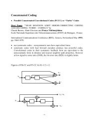
machine. In the recent years so called turbo codes have been a popular research topic, since they
actually can reach very close to Shannon limit. Turbo codes are based on parallel or serial
concatenation of basic (convolutional) codes and they were introduced by Berrou et al. 1993 [2].
The benefit of channel coding is usually given as coding gain, which is the difference in SNR
between uncoded and coded systems at a certain BER level. Unfortunately, this gain is often very
difficult to calculate analytically (at least in realistic situations), thus the performance is usually
found out by computer simulations.
8

A. Block Codes
In general, a block channel encoder takes a block of k information bits in and adds n-k parity
bits in the end of block, thus providing as output n-bit block, which is called a codeword. These
codewords should be carefully designed, so that the channel decoder can recover the original
message, although some transmission errors may have occurred. Hence, the decoder can detect
and correct transmission errors, which improves the average bit error rate in the receiver. This kind
of coding methods are called forward error correction (FEC) schemes. To design a specific FEC
scheme, one has to choose values n and k, develop a good encoding method to construct parity
bits and select a decoding algorithm.
Of course when n is large compared to k, the code makes it possible to detect and correct
several transmission errors within a data block. The decoder just compares the received codeword
to all possible words and selects the best match. If d min is the minimum Hamming distance between
any pair of words, the code can recover all words having t or less errors, where
d min
⎢ −1⎥
t = ⎢ ⎥ . (11)
⎣ 2 ⎦
The code designer tries to maximise minimum distance d min but also the code efficiency R = k/n.
Large n values would be beneficial in design, but unfortunately they lead to complex
implementation of encoder and decoder, and therefore rather small values are usually favoured.
One simple example of generating a (7,4) binary block code is given as a shift register in Fig.4
The upper row is filled with input signal and then the parity bits in the lower row can be calculated.
Finally, all 7 bits are available at the output.
Input data
x 4
x 3
x 2
x 1
+ + +
Output data
c 7
c 6
c 5
Figure 4. Shift register for generating binary (7,4) code. [3]
Channel decoders for block codes are much more complex than encoders due to transmission
errors. A simple comparison between all possible code words and the received word becomes
impractical as the block length grows. Therefore different computationally efficient but still
9

easonably well performing decoding algorithms are developed. Part of the decoding methods are
nonalgebraic procedures, while some others exploit algebraic structure of the code. Decoding
performance improves further, if the decoder can use soft values as input. A soft value tells the
decision bit, but also reliability information on that. For example, value 0.8 can denote strong
probability of transmitting 1 and –0.9 strong probability of sending 0.
B. Convolutional Codes
In contrast to block codes, convolutional codes are operating with continuous stream of input
data instead of blocks. However, they are also based on the redundancy, which distinguish
different codes from each other and enables decoder to detect the correct transmitted sequence.
The convolutional decoders itself differ very much from block decoders, but they are still
characterised by a bit rate R=k/n and a distance measure between codes called minimum free
distance d f , which tells how far apart all possible sequences lie from each other.
So convolutional codes introduce some memory in the transmitted sequence, which is easy to
find from the Fig. 5 below. This encoder takes k=2 bits in at the time and outputs n=3 each time.
What is more, the same inputs are used to provide two sets of outputs; so called constraint length
L is also 2. Typically, k and n are between 1 to 8, and R is then between 1/3 (at least in data
services) and 7/8 and L is from 2 to 10. The convolutional codes are usually expressed with
polynomials that tell which inputs are added in each output. For instance, generator polynomials for
the given (2,3)-code would be 1+D 2 +D 3 , 1+D+D 3 and 1+D 2 , where D means one bit delay variable.
+
Input data
Output data
+
+
Figure 5. A 2/3-rate convolutional encoder with L=2, k=2, n=3. [3]
10

Alternative ways to describe encoder structure is to use state or trellis diagrams[3]. State
diagram shows the internal state of the encoder memory and its possible movements as time goes
by. Trellis diagram is more thorough, since it actually shows all the possible paths (movements), as
it presents each time instant on the right of the current time instant. In that way, the whole trellis is
saved when time goes on. Trellis diagram is especially handy, if one likes study what happens in
the decoding of the sequence.
The decoding problem of convolutional codes (and closely related equalisation problems) is
widely researched area. The two most common approaches (which are also very closely related)
are called the maximum-likelihood sequence estimation MLSE (usually implemented by the Viterbi
algorithm) and maximum a posteriori algorithm MAP. These are briefly introduced in the following,
more information is found for instance from [5] about MLSE and from [4] about MAP.
The MLSE problem is to find the sequence of transmitted information symbols û, which
maximises the likelihood function as follows
( cˆ
u)
uˆ
= arg max p , (12)
u
where ĉ is the received (encoded) signal from the equaliser. An equivalent problem is to maximise
the log-likelihood function log p(c|u), which is solved by minimising the path metric
PM
=
2 ˆ
( ) 2
c ˆ − UΨ
= ∑ c k
− t k
(13)
k
where the reconstructed encoder output assuming structure Ψ is given as
M
∑∑
− 1 L
m= 0 l=
0
t = u g . (14)
k
m,
k−l
m,
l
In MLSE-VA the trellis is spanned by all the L symbols in (14) and each transition is comprised
of M elements, which are describing different encoder outputs. Hence, MLSE finds minimum
sequence error.
The objective of the MAP algorithm is to minimise the bit error probability for each bit by
estimating a posteriori probabilities (APP) of states and transitions of the Markov source from the
received signal sequence. The MAP algorithm introduced by Chang and Hancock [4] uses the
information of the whole received sequence to estimate a single bit probability. In other words, the
MAP algorithm selects the bit ∈{ −1 , + 1}
uˆ
k
u at time instant k, which maximises the following APP
k
[ p( u ĉ)
]
= arg max . (15)
uk
k
The optimum MAP algorithm saves multiplicative transition probabilities in the trellis, which is
computationally difficult. Therefore in practical implementations the path metric is calculated in the
11

log-domain, which enables cumulative calculations. Since MAP requires both forward and
backward recursions, it is around two times more complex than MLSE-VA. The main advantage of
the MAP algorithm is more reliable soft information, since it is optimised for symbolwise decoding.
C. Example (GSM Speech)
To illustrate the two channel coding techniques the coding scheme of GSM Full Rate Speech is
presented in Fig. 6 [6]. The most important beginning of the speech block is protected by block
coding, so there is 3 parity bits for 50 first bits and 4 parity bits for the next 132 bits. Then these
189 bits are protected by ½-rate convolutional code. Finally, 78 last bits are added to the end as
such, because the end is not so important for human's ear.
20 ms of speech
260
BLOCK CODING
50 132 78
50 3 132 4
CONVOLUTIONAL
CODING
189
378 78
456
Figure 6. Coding scheme for GSM Full Rate Speech.
D. Interleaving, nonbinary codes, concatenation
In the presence of bursty error patterns, like in fading channels or interference, the normal error
control methods are not sufficient enough to recover transmission errors. There are three different
ways to improve coding results in this kind of situation; interleaving, nonbinary codes and
concatenation of several codes. A new research topic has also been iterative decoding and
equalisation, which can provide significant gains in some cases.
Interleaving is a simple method to break bursty errors far apart from each other. The bits of a
radio block are simply reordered, which enables decoder to detect and correct transmission errors,
12

ecause errors are not any more consecutively. Like in Fig. 3 is presented, interleaving is done
right after encoding and deinterleaving just before decoding. Block interleaver structure for (15,7)
code with m=5 and d min = 5 is shown in Fig. 7, although convolutional structures are also possible.
So channel coding system with this kind of block interleaving, where bits are read in row after row
and read out column after column (m bits in each column) can cope with up to
⎢d −1⎥
t = m min
⎢ ⎥
(16)
⎣ 2 ⎦
errors. The cost of interleaving is the inevitable delay and storage requirements both in the
transmitter and receiver side.
Output data
Input data
1
6
36
41
66
71
2
7
37
42
67
72
3
8
...
38
43
...
68
73
4
9
39
44
69
74
5 10 40 45
70
75
Figure 7. A block interleaver structure for a (15,7) code with m = 5 and d min = 5.
When nonbinary codes are used, there are more than 2 symbols available to be selected.
Usually there are q=2 k different symbols, which means that k information bits are mapped into one
of those q symbols. The most popular class of nonbinary codes are Reed-Solomon (RS) codes,
which have the following parameters for (N,K) code
• N = q - 1 = 2 k - 1
• K < N
• D min = N - K + 1.
Hence, an (N,K) RS code can correct up to (N-K)/2 symbol errors per block. RS codes are used a
lot due to their good distance properties and efficient decoding algorithms. Also bursty errors lead
to a small number of symbol errors, which often are easy to correct as long as there are less than
(N-K)/2 symbol errors to be corrected.
13

Concatenated code means a combination of two shorter codes that are either serially or parallel
combined, in Fig.8 serially concatenated system is presented. Often the outer code is nonbinary
and inner is binary, like the inner is (n,k) binary convolutional code and outer is (N,K) RS code. The
inner decoder then outputs soft or hard outputs onto k-bit symbols of the outer code. The minimum
distance for the concatenated code is d min D min , where d min and D min are the minimum distances of
the inner and outer codes. The bit rate is Kk/Nn. Also interleaver can be used between outer and
inner coders to handle bursty errors.
Signal
source
Outer
encoder
Inner
encoder
Modulator
Multipath
channel
noise
Outer
decoder
Inner
decoder
Equaliser
Receiver
filter
Figure 8. Block diagram of a system with serially concatenated code.
E. Simulation of coded system
Coded communication link can be divided into two independent parts; the encoder/decoder pair
(codec) and the discrete channel between them. By this way we achieve an efficient and flexible
simulation platform. Typical reason for this separation is that we need 4-16 samples per symbol to
represent the discrete channel, but for codec only one sample per symbol is enough. And if we like
to try another codec with the same discrete channel, it is enough to simulate it with the symbol
rate, which provides computational savings compared to sampling rate. Also this separation
provides useful system insight for the system engineer.
The explicit simulation of a codec is not always needed, since one can approximate or calculate
bounds for the codec performance. There are two clear advantages, if one can avoid simulation.
Decoding algorithms are often very complex and therefore simulations would take a lot of time.
Another thing is that the target bit error probability is set to very low level (like 10 -6 or even lower).
Hence, to achieve confidence in the estimated error rate, we need to simulate at least 10/p
symbols, where p is BER of the system. So the simulation time will be very long. Due to these
reasons codec simulation times are often reduced by statistical means or even calculated
analytically. We can derive quite good bounds for large SNR values and simulate shorter runs for
smaller SNR values. Sometimes an explicit simulation of a codec is required, if for instance some
parameter influence on the decoder is studied.
14

IV. Summary
In this report we have considered source and channel coding methods and how to simulate
them. Source encoding starts with sampling an analog audio signal, then quantization and
encoding into bit groups. In the receiver the digital signal is decoded and filtered back to analog
form. In uniform quantization the input signal is divided into equal intervals, while in nonuniform
methods unequal intervals are used. If correlated sequence is processed, it is useful to exploit
differential quantization. Shannon’s proposal for encoding discrete information is described. That
method allocates shorter codes for messages of higher probability, thus the average number of bits
per symbol decreases. Usually it is enough to simulate idealized and very simple A/D converter,
although real converter has many imperfections. With this assumption, we can actually replace
source encoding with (pseudo) random binary sequence in the simulation.
Channel coding is used to achieve more reliable transmission by adding parity check bits after
information bits. Typical channel encoding techniques are block and convolutional codes. The
block encoders are processing a block of data at a time and calculating the parity check bits for this
block. A code designer tries to maximise the minimum Hamming distance between any pair of
code words, but also transmit as little redundancy bits as possible. Convolutional encoders
introduce memory into the code by using the previous time instants as well to calculate the current
encoder output. Convolutional decoders are often based on MLSE principle, which finds the
minimum sequence error, or on MAP principle, which solves the minimum symbol error. For
instance in Full Rate GSM Speech both block and convolutional encoding are used, but on the
other hand, the end of each burst is kept uncoded as it is not so critical for human’s ear. Another
methods to improve link performance is to use interleaving, nonbinary codes (more than 2 different
symbols available) or concatenate at least two codes serially or parallel.
The coded system consists of encoder/decoder pair and a discrete channel between them.
Typically several samples per symbol are needed to represent the channel part in a simulation, but
only one sample per symbol in the codec. Sometimes it is enough to calculate bounds for a coded
system and thereby avoid long and complex simulations. Especially for high SNR values one can
calculate reliable bounds and save a lot of simulation time.
15

V. References
[1] M. C. Jeruchim, P. Balaban, and K. S. Shanmugan, "Simulation of Communication Systems",
Plenum Press, 1992, 731 p.
[2] C. Berrou, A. Glavieux and P. Thitimajshima, "Near Shannon Limit Error-Correcting Coding
and Decoding: Turbo-Codes", Proc. ICC’93, Geneva, Switzerland, May 1993, pp. 1064-1070.
[3] J.G. Proakis, "Digital Communications", 3 rd edition, McGraw-Hill, 1995, 929 p.
[4] R.W. Chang and J.C. Hancock, “On Receiver Structures for Channels Having Memory”, IEEE
Trans. on Inf. Theory, Vol. 12, No. 3, pp. 463-468, Oct. 1996.
[5] G. D. Forney, Jr., "Maximum-likelihood Sequence Estimation of Digital Sequences in the
Presence of Intersymbol Interference", IEEE Trans. Inf. Theory, Vol. IT-18, pp. 363-378, May
1972.
[6] ETSI specifications, GSM 05.03, Channel coding, March 1995.
16

VI. Homework
P4.20. Discrete Channel Model and Coding. Parity-check codes are frequently used in data
communications. In each byte (8 bits), 7 bits represents information and the eighth is a parity bit; it
is "1" if the number of "ones" in the information bits is odd, and it is "0" otherwise. Thus, the
number of "ones" in every byte should be even and the receiver detects errors if the number of
"ones" is odd. Find the probability of undetected errors for the Gilbert model given below (See ex.
4.3 and 4.4).
Gilbert model. According to Gilbert’s model, it consists of stochastic sequential machine (SSM),
which has two states: G (good) and B (bad) with transition probabilities
q 11 = 0.997, q 12 = 0.003, q 21 = 0.034, q 22 = 0.966.
The model state transition diagram is illustrated in Fig. 9 below. In state G errors do not occur,
while in state B the bit-error probability equals 0.16. Thus we have
p 00 (1) = 1, p 01 (1) = 0, p 10 (1) = 0, p 11 (1) = 1
p 00 (2) = 0.84, p 01 (2) = 0.16, p 10 (2) = 0.16, p 11 (2) = 0.84.
0.003
0.997 G
B
0.966
0.034
0
1.0
0
0
0.84
0
0.0
0.16
1
1.0
1
1
0.84
1
p ij
(G)
p ij
(B)
Figure 9. Gilbert model, state and channel transitions.
17