Fuzzy sliding mode control for discrete nonlinear systems

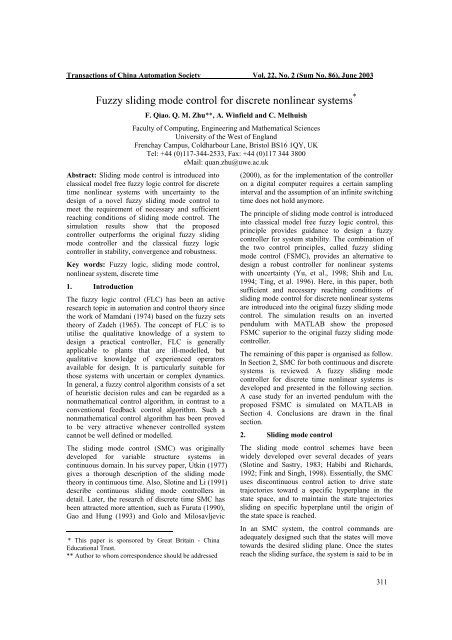
Transactions of China Automation Society Vol. 22, No. 2 (Sum No. 86), June 2003
Fuzzy sliding mode control for discrete nonlinear systems *
F. Qiao. Q. M. Zhu**, A. Winfield and C. Melhuish
Faculty of Computing, Engineering and Mathematical Sciences
University of the West of England
Frenchay Campus, Coldharbour Lane, Bristol BS16 1QY, UK
Tel: +44 (0)117-344-2533, Fax: +44 (0)117 344 3800
eMail: quan.zhu@uwe.ac.uk
Abstract: Sliding mode control is introduced into
classical model free fuzzy logic control for discrete
time nonlinear systems with uncertainty to the
design of a novel fuzzy sliding mode control to
meet the requirement of necessary and sufficient
reaching conditions of sliding mode control. The
simulation results show that the proposed
controller outperforms the original fuzzy sliding
mode controller and the classical fuzzy logic
controller in stability, convergence and robustness.
Key words: Fuzzy logic, sliding mode control,
nonlinear system, discrete time
1. Introduction
The fuzzy logic control (FLC) has been an active
research topic in automation and control theory since
the work of Mamdani (1974) based on the fuzzy sets
theory of Zadeh (1965). The concept of FLC is to
utilise the qualitative knowledge of a system to
design a practical controller, FLC is generally
applicable to plants that are ill-modelled, but
qualitative knowledge of experienced operators
available for design. It is particularly suitable for
those systems with uncertain or complex dynamics.
In general, a fuzzy control algorithm consists of a set
of heuristic decision rules and can be regarded as a
nonmathematical control algorithm, in contrast to a
conventional feedback control algorithm. Such a
nonmathematical control algorithm has been proved
to be very attractive whenever controlled system
cannot be well defined or modelled.
The sliding mode control (SMC) was originally
developed for variable structure systems in
continuous domain. In his survey paper, Utkin (1977)
gives a thorough description of the sliding mode
theory in continuous time. Also, Slotine and Li (1991)
describe continuous sliding mode controllers in
detail. Later, the research of discrete time SMC has
been attracted more attention, such as Furuta (1990),
Gao and Hung (1993) and Golo and Milosavljevic
* This paper is sponsored by Great Britain - China
Educational Trust.
** Author to whom correspondence should be addressed
(2000), as for the implementation of the controller
on a digital computer requires a certain sampling
interval and the assumption of an infinite switching
time does not hold anymore.
The principle of sliding mode control is introduced
into classical model free fuzzy logic control, this
principle provides guidance to design a fuzzy
controller for system stability. The combination of
the two control principles, called fuzzy sliding
mode control (FSMC), provides an alternative to
design a robust controller for nonlinear systems
with uncertainty (Yu, et al., 1998; Shih and Lu,
1994; Ting, et al. 1996). Here, in this paper, both
sufficient and necessary reaching conditions of
sliding mode control for discrete nonlinear systems
are introduced into the original fuzzy sliding mode
control. The simulation results on an inverted
pendulum with MATLAB show the proposed
FSMC superior to the original fuzzy sliding mode
controller.
The remaining of this paper is organised as follow.
In Section 2, SMC for both continuous and discrete
systems is reviewed. A fuzzy sliding mode
controller for discrete time nonlinear systems is
developed and presented in the following section.
A case study for an inverted pendulum with the
proposed FSMC is simulated on MATLAB in
Section 4. Conclusions are drawn in the final
section.
2. Sliding mode control
The sliding mode control schemes have been
widely developed over several decades of years
(Slotine and Sastry, 1983; Habibi and Richards,
1992; Fink and Singh, 1998). Essentially, the SMC
uses discontinuous control action to drive state
trajectories toward a specific hyperplane in the
state space, and to maintain the state trajectories
sliding on specific hyperplane until the origin of
the state space is reached.
In an SMC system, the control commands are
adequately designed such that the states will move
towards the desired sliding plane. Once the states
reach the sliding surface, the system is said to be in
311

Transactions of China Automation Society Vol. 22, No. 2 (Sum No. 86), June 2003
sliding mode. During the sliding mode, the system s ( t)
s& ( t)
< 0
(2.5)
possesses some invariance properties, such as
where s& (t)
represents the time derivative of s (t)
.
robustness, order reduction and disturbance rejection.
The first step to design a sliding mode control is to
determine the sliding hyperplane with desired
dynamics of the corresponding sliding motion. And
the next step is to design the control input so that the
state trajectories are driven and attracted toward the
sliding hyperplane and then remained sliding on it
for all subsequent time.
In the following, the sliding mode control for
continuous and discrete time system is reviewed.
2.1 Continuous sliding mode control
For a single input and single output continuous
nonlinear system with n state variables, the
companion form is as follow,
( )
x& n ( t)
= f ( X ( t))
+ b(
X ( t))
u(
t)
+ d(
t)
(2.1a)
and
y ( t)
= x(
t)
, for t ≥ 0
(2.1b)
where the state vector is
( n−1)
T
X ( t)
= [ x(
t),
x& ( t),
L x ( t)]
, u(t)
is the control
input, y(t)
is the system output and d(t)
is an
external disturbance. If the reference output is y r
(t)
,
the above dynamic equations can be transferred into
the following state equations with error signal
e1 ( t)
= y(
t)
− y
r
( t)
and its derivatives as state
variables:
e&
1
( t)
= e2
( t)
e&
2
( t)
= e3
( t)
for t > 0 .(2.2)
M
e&
n
( t)
= f ( E(
t))
+ b(
E(
t))
u(
t)
+ d(
t)
Let E( t)
= [ e1 ( t),
e2
( t),
L en ( t)]
∈ R and δ ∈ R . A
linear functional s : E → δ is defined by
s ( t)
= CE(
t)
(2.3)
where C = [ c1,
c2,
L cn−
1,1]
( ci
s are all real numbers).
Then, a sliding hyperplane can be represented as
s( t)
= 0 or
c e t)
+ c e ( t)
+ L + e ( t)
0
(2.4)
1
(
1 2 2
n
=
The scalar s (t)
of (2.3) is defined as the distance to
the s (t)
hyperplane of (2.4).
The motion sliding on the sliding hyperplane is
commonly referred to as a sliding mode. If the
following condition is satisfied with the designed
control input, the just mentioned requirements on the
state trajectories can be fulfilled:
Inequality of (2.5) is called the reaching condition
of sliding control for continuous systems under
which the state will move toward and reach a
sliding surface.
If the control input is so designed that the
inequality s ( t)
s& ( t)
< 0 is satisfied, together with
the properly chosen sliding hyperplane, the state
will be driven toward the origin of the state space
along the sliding hyperplane from any given initial
state. This is the way of the SMC that guarantee
asymptotic stability of the systems.
2.2 Discrete sliding mode control
The implementation of the controller on a digital
computer requires a certain sampling interval and
the assumption of an infinite switching time does
not hold anymore. Milosavljevic (1985) derived
conditions which ensure the existence of a sliding
mode in discrete time, the so-called quasi-sliding
mode. Techniques of designing sliding mode
controller for discrete time domain were proposed
by Drakunov and Utkin (1989) and Furuta (1990).
Golo and Milosavljevic (2000) proposed a new
design for discrete time SMC. Sira-Ramirez (1991)
investigated sliding mode controllers for discrete
nonlinear. The systems, however, that can be
controlled are subject to strong restrictions.
The discretisation form of (2.1) with first order
approximation is as follow
x1
( k + 1) = x1
( k)
+ Tx2
( k)
x2
( k + 1) = x2
( k)
+ Tx3
( k)
M
xn−
1(
k + 1) = xn−
1(
k)
+ Txn
( k)
xn
( k + 1) = xn
( k)
+ Tf ( X ( k))
+ Tb(
X ( k))
u(
k)
+ Td(
t)
(2.8a)
and
y ( k ) = x ( k ) , for k = 0,1T
, 2T
, L,
1
nT , (2.8b)
(T is the sampling rate)
T
where X ( k)
= [ x ( k),
x ( k),
x ( k)]
1 2
L
n
.
s(k)
is defined similar to that in continuous time
domain
s ( k)
= CX ( k).
(2.9)
where C = [ c , c , L c ,1]
(
1 2 n−1
ci
s are all real
numbers). s ( k)
= 0 is the so-called hyperplane
which is equivalent to the sliding surface in
continuous time. Since it cannot be ensured that the
312

Transactions of China Automation Society Vol. 22, No. 2 (Sum No. 86), June 2003
states remain on the surface for all time because of of SMC. Here, an FSMC for discrete nonlinear
the discretisation, it is also called quasi-sliding mode. systems is proposed.
Again, C is chosen such that the system is
For the discrete time system (2.8), assume that the
asymptotically stable while being on the hyperplane.
sliding surface is
n
One way to evaluate C is to use the pole placement
s( k)
=
method. The system has to be written in its ∑ ci
xi
( k)
(3.1)
i=
1
controllability canonical form and the final state can
where c
be represented in terms of remaining when staying
i
> 0,
i = 1,2, L,
n . And we can get
on the sliding surface S .
So from (2.10), the necessary reaching condition is
as follow
In discrete case, discretisation form of (2.5) will be s(
k)(
s(
k + 1) −s(
k))
s ( k)[
s(
k + 1) − s(
k)]
< 0
(2.10)
n
n
n
⎛
⎞
This is the necessary reaching condition for the = ∑ci
xi
( k)
⎜∑ci
xi
( k + 1) −∑ci
xi
( k)
⎟
i= 1
sliding mode control, it only makes the sliding
⎝ i=
1
i=
1 ⎠
(3.2)
n
n
motion toward the sliding surface.
= ∑ci
xi
( k)(
∑ci
xi+
1(
k)
+
In order to satisfy the reaching, the following
i=
1
i=
1
inequality has to be satisfied to meet the requirement cn
f ( X(
k))
+ cnb(
X(
k))
u(
k)
+ cnd(
k))
T < 0
of the sufficient reaching condition for the existence Suppose that c n
is positive and b (X ) is negative,
of a sliding motion, too
(3.2) presents that as s (k)
is positive, increasing
s ( k + 1) < s(
k)
(2.11)
The combination of (2.10) and (2.11) can make sure
the sliding motion convergent.
Just as in continuous time, in discrete time,
equivalent control u eq
(k)
is designed to try to keep
the system on sliding surface which is represented as
s ( k + 1) = s(
k)
(2.12)
and the switching term, u s
(k)
, is designed to (satisfy
the reaching condition (2.10) and (2.11)) overcome
the external disturbance and reaching the stable state.
However, the most disadvantage of using SMC is the
chattering phenomenon. Because a discontinuous
switching control is applied to the plant, chattering
always appears as a source to excite the unmodelled
high frequency dynamics of the controlled system.
One commonly used method to eliminate the
chattering is to replace the relay control by a
saturating approximation. Another method is to
apply fuzzy logic control to the SMC system such
that a smooth and reasonable hitting control can be
generated to reduce the chattering.
3. Fuzzy sliding mode control
It is difficult to design a sliding mode controller for
nonlinear system. Up to now, there have been quite a
lot of research on the combination of sliding mode
control with fuzzy logic control techniques for
improving the robustness and performance of
nonlinear systems with uncertainty (Chen and Chang,
1998; Li and Shieh, 2000; Wang et al, 2001, a, b; and
Chang et al. 2002).
The purposed fuzzy control is called fuzzy sliding
mode control (FSMC) as it is based on the principle
u (k) will result in decreasing s( k)(
s(
k + 1) − s(
k))
,
and that as s (k)
is negative, decreasing u(k)
will
result in decreasing s( k)(
s(
k + 1) − s(
k))
. On the
other hand, suppose c n
b(X ) is positive, (3.2)
denotes that decreasing u (k)
will cause decreasing
s( k)(
s(
k + 1) − s(
k))
as s (k ) is positive, and
increasing u (k)
will cause decreasing
s( k)(
s(
k + 1) − s(
k))
as s (k ) is negative.
Therefore, all such statements above can be
summarised as a fuzzy rule base used in FLC. (The
design of a fuzzy sliding mode controller is
detailed in Section 4.)
Note that the control law should meet the
requirement for the sufficient reaching condition
(2.11) too.
4. FSMC for inverted pendulum
4.1 System description
The inverted pendulum is often used as a
benchmark for all kinds of controllers. It is a
nonlinear, unstable system which makes it
challenge to control. The system is composed of
a rigid pole and a cart on which the pole is
hinged to the cart through a pivot such that it has
only one degree of freedom. The goal of the
control is to make the pole upright. The dynamic
model equations for the plant are
M & x&+
N = u
(4.1)
&2
N = mx &
+ ml && θ cosθ
− mlθ
sinθ
(4.2)
2
P − mg = −ml(
& θ
sinθ
+ & θ cosθ
) (4.3)
313

Transactions of China Automation Society Vol. 22, No. 2 (Sum No. 86), June 2003
I θ
= Pl sinθ
− Nl cosθ
⎡ ml cos x1 ( k)
⎤
b = −T
⎢
0
2
2 ⎥ <
where M is the mass of the cart, m is the mass of
⎣(
M + m)(
ml + I)
− ( ml cos x ( k))
1 ⎦
,
2
the of the pendulum, I = ( 1/3) ml is the moment π π
for − < x
1(
k)
<
of the inertia of the pendulum, θ is the angular
2 2
position of the pendulum deviated from the which is the same as assumption in (3.2). Then the
equilibrium position, x is the position of the cart, fuzzy rules described in Section 3 are further
l is the half length of the pendulum. The system detailed as follow
friction is omitted for simplicity.
1) If s( k)
> 0 and − s ( k)
< s(
k + 1) < s(
k)
, increasing
The dynamic equation of θ can be rewritten as u(k)
will strengthen (4.9) and meet the sufficient
2
2
( M + m)(
ml + I)
− ( ml cosθ
) && θ +
condition (4.10).
2) If s( k)
> 0 and s ( k + 1) > s(
k)
, greatly increasing
[ ]
2
( ml & θ ) cosθ
sinθ
−
( M + m)
ml sinθ
+ ml cosθu
= 0
(4.5)
If we define x = θ and x = & θ , then the first order
1
2
approximation of the plant plus zero order hold for
the sampling representative of (4.5) can be expressed
as
x1
( k + 1) = x1(
k)
+ Tx2(
k)
⎡ ( M + m)
mlgsin
x1(
k)
x2(
k + 1) = x2(
k)
+ T ⎢
2
⎣(
M + m)(
ml + I)
− ( ml cos x1
( k))
2
( mlx1
( k))
cos x1(
k)sin
x1
( k)
−
2
2
( M + m)(
ml + I)
− ( ml cos x1(
k))
ml cos x
⎤
1(
k)
u(
k)
−
2
2 ⎥
( M + m)(
ml + I)
− ( ml cos x1(
k))
⎦
(T is the sampling rate).
4.2 Controller design
2
(4.6)
The expression for the linear functional s(k)
is
chosen as
s ( k)
= c1x1
( k)
+ x2
( k)
(4.7)
The corresponding sliding hyperplane is represented
by
s ( k)
= c1 x1
( k)
+ x2
( k)
= 0
(4.8)
Review the necessary and sufficient reaching
conditions,
s ( k)(
s(
k + 1) − s(
k))
< 0
(4.9)
and
s ( k + 1) < s(
k)
(4.10)
S , ∆ S , ∆ S and ∆ U are the fuzzy variables of
s (k) , ( s( k + 1) − s(
k)
) , s( k + 1) − s(
k)
and control
variable increment ∆ u , respectively. The
membership functions for S , ∆ S , ∆ S and ∆U
are
chosen to be in the shape of triangular type.
From (4.6), we can know
u (k) will be helpful to reach the conditions of (4.9) and
(4.10).
3) If s( k)
> 0 and s( k + 1) < −s(
k)
, reasonably
decreasing u (k)
will be helpful to meet the sufficient
reaching requirement of (4.10).
4) If s( k)
< 0 and s( k)
< s(
k + 1) < −s(
k)
,
decreasing u (k)
will strengthen (4.9) and meet the
sufficient condition (4.10).
5) If s ( k)
< 0 and s( k + 1) > −s(
k)
, greatly
increasing u (k)
will be helpful to meet (4.10).
6) If s ( k)
< 0 and s ( k + 1) < s(
k)
, reasonably
decreasing u (k)
will be helpful to meet (4.9) and (4.10).
4.3 Simulation results
The parameters of the inverted pendulum for
simulation are l = 0. 5m
, M = 2kg
and m = 0. 3kg
.
And the coefficient c 1
is chosen as c = 6 . The
1
initial conditions of the inverted pendulum are
supposed to be: (a) θ = −1
and ω = 1 , and (b)
θ = 0.5 and ω = 1 . At t = 2. 5 second, an external
disturbance with d ( t)
= 20 is added to the
pendulum to verify the robustness of the controller.
The simulation is made on MATLAB, and the
simulation results with the proposed FSMC
(PFSMC) are shown on Figure 4.1 (a) and (b), on
which the simulation results with the original
FSMC (OFSMC) and a classical fuzzy logic
control (FCL) with the same initial conditions and
the same sampling rate are also shown for the
purpose of performance comparison. In Figure 4.2,
the same initial conditions of the inverted
pendulum are set for the simulation, and a
uniformly distributed random noise with 0 mean
and 0.
083 variance is added to the system.
314

Transactions of China Automation Society Vol. 22, No. 2 (Sum No. 86), June 2003
[4]. Fink, A. and Singh, T., (1998), “Discrete sliding
mode controller for pressure control with an
electrohydraulic servovalve”, IEEE Conference on
Control Applications (CCA), Trieste, Italy, pp. 378-382.
[5]. Furuta, K., (1990), “Sliding mode control of a
discrete system”, Systems and Control Letters, pp. 145-
152.
[6]. Gao, W. and Hung, J. C., (1993), “Variable structure
control of nonlinear systems: a new approach”, IEEE
Transaction IE-40 pp. 43-55.
[7]. Golo, G. and Milosavljevic, C., (2000), “Robust
discrete-time chattering free sliding mode control”,
Systems and Control Letters, 41, pp. 19-28.
[8]. Habibi, S.R. and Richards, R. J., (1992), “Sliding
Figure 4.1 Simulation results without noise mode control of an electrically powered industrial robot”,
IEE Proc. Pt. D., pp207-225.
[9]. Li, T. H. S and Shieh, M. Y., (2000), “Switchingtype
fuzzy sliding mode control of a cart pole system”,
Mechtronics 10, pp. 91-109.
[10]. Mamdani, E. H., (1974), “Applications of fuzzy
algorithms for simple dynamic plants”, Proc. IEE, 121,
pp 1585-1588.
[11]. Milosavljevic, C., (1985), “General conditions for
the existence of a quasisliding mode on the switching
hyperplane in discrete variable structure systems”,
Automatic Remote Control, 46, pp. 307-314.
[12]. Shih, M. C. and Lu, C. S., (1994), “Fuzzy sliding
mode position control of a ball screw driven by
pneumatic servomotor”, Mechtronics, Vol. 5, No. 4,
Figure 4.2 Simulation results with noise
pp.421-431.
[13]. Sira-Ramirez, H., (1991), “Nonlinear discrete
5. Conclusions
variable structure systems in quasi-sliding mode”,
International Journal of Control, pp. 1171-1187.
A fuzzy sliding mode controller is designed in this [14]. Slotine, J. J. E. and Li. W., (1991), “Applied
paper by introducing sliding mode control into fuzzy nonlinear control”, Prentice Hall, Englewood Cliffs, NJ.
logic control for discrete nonlinear systems with [15]. Slotine, J. J. E. and Sastry, S. S., (1983), “Tracking
uncertainty, both the necessary and sufficient control of nonlinear systems using sliding surface with
reaching condition of the sliding mode control are application to robot manipulators”, International Journal
integrated into the controller. The proposed FSMC of Control, pp. 465-492.
overcomes the chattering problem, and speed up the [16]. Ting, C. S., Li, T. H. S, and Kung, F. C., (1996),
“An approach to systematic design of the fuzzy control
convergence compared with the original FSMC. The
system”, Fuzzy Sets and Systems, 77, pp. 151-166.
controller does not need the accurate system
[17]. Utkin, V. I., (1977), “Variable structure systems
mathematical model, so it is relatively easy to design. with sliding mode”, IEEE Transactions on Automatic
The simulation results verify that the proposed Control, Vol. AC-22, No. 2, pp 212-222, April.
controller superior to the original FSMC and the [18]. Wang, J. Rad, A. B. and Chan, P. T., (2001 a),
classical fuzzy logic controller in stability, “Indirect adaptive fuzzy sliding mode control: Part I:
convergence and robustness.
fuzzy switching”, Fuzzy Sets and Systems, 122, pp.21-
30.
References
[19]. Wang, J. Rad, A. B. and Chan, P. T. (2001, b),
[1]. Chang, W., Park, J. B. Joo, Y. H. and Chen, G., (2002),
“Indirect adaptive fuzzy sliding mode control: Part I:
“Design of robust fuzzy-model based controller with
fuzzy switching”, Fuzzy Sets and Systems, 122, pp. 21-
sliding mode control for SISO nonlinear systems”, Fuzzy
30.
Sets and Systems, 125, pp.1-22.
[20]. Yu, X. H., Man, Z. H. and Wu, B. L., (1998),
[2]. Chen, C. L. and Chang, M. H., (1998), “Optimal
“Design of fuzzy sliding-mode control systems”, Fuzzy
design of fuzzy sliding-mode control: a comparative study”,
Sets and Systems, 95, pp.295-306.
Fuzzy Sets and Systems, 93, pp. 37-48.
[21]. Zadeh, L. A., (1965), “Fuzzy sets,” Information
[3]. Draunov, S. V. and Utkin, V. I., (1989), “On discrete
and Control, vol. 8, pp. 338-353.
time sliding modes”, IFAC Nonlinear Control Systems
Design, pp. 273-278.
315