An Introduction to Error Correction Models An Introduction to ECMs ...

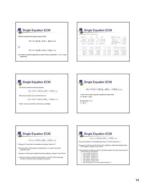
Single Equation ECM
We then estimate the single equation ECM
As
∆Y t = α + β 0∆X t - β 1(Y t-1 - β 2X t-1) + ε t
∆Y t = α + β 0∆X t + β 1Y t-1 + β 2X t-1 + ε t
If our error correction approach is correct, then β 1 should be -1 < β 1 < 0 and
significant.
Single Equation ECM
The results indicate the following equation
∆Y t = 13.12 + 1.32*∆X t -.42*Y t-1 + .52*X t-1 + ε t
Which we can write in error correction form as
∆Y t = 13.12 + 1.32*∆X t -.42(Y t-1 - 1.22*X t-1 ) + ε t
Where 1.22 is our calculation of the long run multiplier
Single Equation ECM
∆Y t = α + 1.32*∆X t -.42(Y t-1 - 1.22*X t-1 ) + ε t
Changes in X have both an immediate and long term effect on Y
When the portion of the equation in parentheses = 0, X and Y are in their
equilibrium state.
Increases in X will cause deviations from this equilibrium, causing Y to be too low.
Y will then increase to correct this disequilibrium, with 42% of the (remaining)
deviation corrected in each subsequent time period.
Single Equation ECM
regress dif_y dif_x lag_y lag_x
Source | SS df MS Number of obs = 55
-------------+------------------------------ F( 3, 51) = 21.40
Model | 238.216589 3 79.4055296 Prob > F = 0.0000
Residual | 189.278033 51 3.71133398 R-squared = 0.5572
-------------+------------------------------ Adj R-squared = 0.5312
Total | 427.494622 54 7.91656707 Root MSE = 1.9265
-----------------------------------------------------------------------------dif_y
| Coef. Std. Err. t P>|t| [95% Conf. Interval]
-------------+---------------------------------------------------------------dif_x
| 1.324821 .200003 6.62 0.000 .9232986 1.726344
lag_y | -.4248235 .1146587 -3.71 0.001 -.6550105 -.1946365
lag_x | .5182186 .1971867 2.63 0.011 .1223498 .9140873
_cons | 13.12112 4.201755 3.12 0.003 4.685745 21.55649
------------------------------------------------------------------------------
Single Equation ECM
∆Y t = 13.12 + 1.32*∆X t -.42(Y t-1 - 1.22*X t-1) + ε t
Y and X are in their long term equilibrium state when
Y = 30.89 + 1.22X
So that when X = 1
Y = 32.11
Single Equation ECM
∆Y t = α + 1.32*∆X t -.42(Y t-1 - 1.22*X t-1 ) + ε t
A one unit increase in X immediately produces a 1.32 unit increase in Y.
Increases in X also disrupt the the long term equilibrium relationship between these
two variables, causing Y to be too low.
Y will respond by increasing a total of 1.22 points, spread over future time periods at
a rate of 42% per time period.
� Y will increase .52 points at t
� Then another .3 points at t+1
� Then another .2 points at t+2
� Then another .1 points at t+3
� Then another .05 points at t+4
� Then another .03 points at t+5
� Until the change in X at t-1 has virtually no effect on Y
14