Taguchi Design Tutorial - Statease.info

DX7-03E-Taguchi.doc Rev. 4/10/06
Taguchi Design Tutorial
Introduction
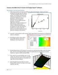
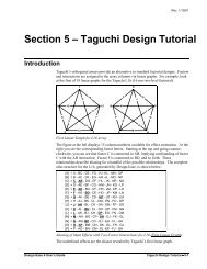
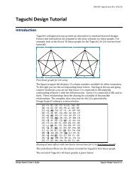
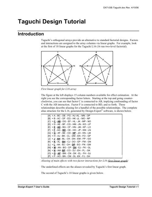
Taguchi’s orthogonal arrays provide an alternative to standard factorial designs. Factors
and interactions are assigned to the array columns via linear graphs. For example, look
at the first of 18 linear graphs for the Taguchi L16 (16 run two-level factorial).
1
A
3
9
14
C
J
O
2
13
15
B
N
P
11
L
6
7
5
F
E
G
10
K
12
4
8
D
M
H
First linear graph for L16 array
The figure at the left displays 15 column numbers available for effect estimation. At the
right you see the corresponding factor letters. Starting at the top and going counterclockwise,
you can see that factor C is connected to AB, implying confounding of factor
C with the AB interaction. Factor F is connected to BD, and so forth. These
relationships describe aliasing for a handful of the possible relationships. The complete
alias structure for the L16, generated by Design-Expert ® software, is shown below.
[A] = A - BC - DE - FG - HJ -KL - MN - OP
[B] = B - AC - DF - EG - HK -JL - MO - NP
[C] = C - AB - DG - EF - HL - JK - MP - NO
[D] = D - AE - BF - CG - HM - JN - KO - LP
[E] = E - AD - BG - CF - HN - JM - KP - LO
[F] = F - AG - BD - CE - HO - JP - KM - LN
[G] = G - AF - BE - CD - HP - JO - KN - LM
[H] = H - AJ - BK - CL - DM - EN - FO - GP
[J] = J - AH - BL - CK - DN - EM - FP - GO
[K] = K - AL - BH - CJ - DO - EP - FM - GN
[L] = L - AK - BJ - CH - DP - EO - FN - GM
[M] = M - AN - BO - CP - DH - EJ - FK - GL
[N] = N - AM -BP - CO - DJ - EH - FL - GK
[O] = O - AP - BM - CN - DK - EL - FH - GJ
[P] = P - AO - BN - CM - DL -EK - FJ - GH
Aliasing of main effects with two-factor interactions for L16 (first linear graph)
The underlined effects are the aliases revealed by Taguchi’s first linear graph.
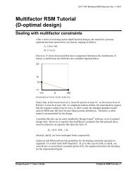
The second of Taguchi’s 18 linear graphs is given below.
Design-Expert 7 User’s Guide Taguchi Design Tutorial • 1

9
J
3
1
14
C
A
O
10
13
7
K
N
G
11
L
6
15
5
2
F
E
B
P
4
12
8
M
D
H
Second linear graph for L16
This second linear graph reveals the underlined, italicized effects shown below.
[A] = A - BC - DE - FG - HJ - KL - MN - OP
[B] = B - AC - DF - EG - HK - JL - MO - NP
[C] = C - AB - DG - EF - HL - JK - MP - NO
[D] = D - AE - BF - CG - HM - JN - KO - LP
[E] = E - AD - BG - CF - HN - JM - KP - LO
[F] = F - AG - BD - CE - HO - JP - KM - LN
[G] = G - AF - BE - CD - HP - JO - KN - LM
[H] = H - AJ - BK - CL - DM - EN - FO - GP
[J] = J - AH - BL - CK - DN - EM - FP - GO
[K] = K - AL - BH - CJ - DO - EP - FM - GN
[L] = L - AK - BJ - CH - DP - EO - FN - GM
[M] = M - AN - BO - CP - DH -EJ - FK - GL
[N] = N - AM - BP - CO - DJ - EH - FL - GK
[O] = O - AP - BM - CN - DK - EL - FH - GJ
[P] = P - AO - BN - CM - DL - EK - FJ - GH
Aliasing of main effects with two-factor interactions for L16 (second linear graph)
In theory, you could build the entire alias structure by going through all 18 linear graphs.
But, why bother The complete alias structure is given by Design-Expert software via
its Design Evaluation tool.
Case Study
To see how Design-Expert software handles Taguchi arrays, let’s look at a welding
example out of System of Experiment Design, Volume 1, page 189 (Quality Resources,
1991). The experimenters identified nine factors (see table below).
2 • Taguchi DesignTutorial Design-Expert 7 User’s Guide

DX7-03E-Taguchi.doc Rev. 4/10/06
Factor Units Level 1 Level 2
Brand J100 B17
Current amps 150 130
Method weaving single
Drying none 1 day
Thickness mm 8 12
Angle degrees 70 60
Stand-off mm 1.5 3.0
Preheat none 150 deg C
Material SS41 SB35
Factors for welding experiment
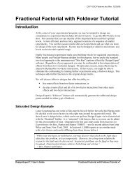
The experimenters wanted estimates of several interactions: AB, AD and BD. Looking
at the first L16 linear graph (reproduced in part below), we see that column C can be
used to estimate the AB interaction, column E to estimate AD, column F to estimate BD
and column O to estimate AP. Taguchi used columns M and N to estimate error.
1
A
3
14
C
O
2
15
B
P
6
5
F
E
4
Subset of first linear graph for L16 on welding
The factor assignments are summarized below.
Column Factor Column Factor
A
Brand
B Current J Angle
C AB K Stand-off
D Method L Preheat
E AD M
F BD N
G Drying O AP
H Thickness P Material
Factor assignments for L16 on welding
D
Design-Expert 7 User’s Guide Taguchi Design Tutorial • 3

Columns M and N (blank) will be used to estimate error. (Note: there is no column
labeled “I” in this or other designs because this is reserved for the intercept of the
predictive model.)
Design the Experiment
Let’s build this design. Choose File, New Design off the menu bar. (The blank-sheet
icon on the left of the toolbar is a quicker route to this screen. If you’d like to check
this out, press Cancel to re-activate the tool bar.) Then from the default Factorial tab
click Taguchi OA and choose L16(2^15) from the pull down menu.
Selecting the Taguchi orthogonal array (OA)
Click on the Continue button. The software then presents the alias structure for the
chosen design. Notice that C is aliased with AB, E is aliased with AD, F is aliased with
BD and O is aliased with AP. Also, Design-Expert reserves the letter “I” for the
intercept in predictive models, so it skips from factor “H” to “J.”
[A] = A - BC - DE - FG - HJ - KL - MN - OP
[B] = B - AC - DF - EG - HK - JL - MO - NP
[C] = C - AB - DG - EF - HL - JK - MP - NO
[D] = D - AE - BF - CG - HM - JN - KO - LP
[E] = E - AD - BG - CF - HN - JM - KP - LO
[F] = F - AG - BD - CE - HO - JP - KM - LN
[G] = G - AF - BE - CD - HP - JO - KN - LM
[H] = H - AJ - BK - CL - DM - EN - FO - GP
[J] = J - AH - BL - CK - DN - EM - FP - GO
[K] = K - AL - BH - CJ - DO - EP - FM - GN
[L] = L - AK - BJ - CH - DP - EO - FN - GM
[M] = M - AN - BO - CP - DH - EJ - FK - GL
[N] = N - AM - BP - CO - DJ - EH - FL - GK
[O] = O - AP - BM - CN - DK - EL - FH - GJ
[P] = P - AO - BN - CM - DL - EK - FJ - GH
Alias structure for L16 two-level design (2 15 )
4 • Taguchi DesignTutorial Design-Expert 7 User’s Guide

DX7-03E-Taguchi.doc Rev. 4/10/06
Click on the Continue button. On all other designs you would now be prompted to
enter factor names. However, for Taguchi designs this will be done later, after you
generate the layout of runs. Design-Expert now shows the response screen. Enter the 1
response name as “Tensile” and the units as “kg/mm^2”.
Response entry
Click on the Continue button. Design-Expert now displays the design in random order.
Right click on the Std column and choose Sort by Standard Order to see Taguchi’s
design order.
Sorting design by standard order
Next, right click on the heading of column A and choose Edit Info: Enter “Brand” as
the name and “J100” and “B17” as level 1 and level 2. These are nominal (named)
contrasts, so leave that option as the default.
Using Edit Info screen
Design-Expert 7 User’s Guide Taguchi Design Tutorial • 5

The rest of the factors can be entered in the same way, but to save time read in the
response data via File, Open Design from the main menu. Select the file named
Taguchi-L16.dx7.
Recall that several of the columns (C, E, F and O) are being used to estimate interactions.
Two others (M and N) are used to estimate error. We can delete all these
columns and fit the interactions directly. This will greatly simply the analysis.
Right click on the header for column O (Factor 14) to bring up a menu as shown below.
Choose Delete Factor and confirm with a Yes.
Right-Click Menu for Factor Column in Design Layout
When deleting factors, the letters associated with the remaining factors change, so to
avoid confusion, always start at the right and work left. Be patient – it takes the
software a few moments to re-tabulate the design. Also, the focus shifts back to the
leftmost part of the design, so you must scroll back each time to select the next column
for deletion. All this work will eventually pay off by putting you in position to take
advantage of Design-Expert’s powerful analytical capabilities.
Repeat the Delete Factor operation on the columns for factors N, M, F, E and C.
When you finish deleting columns, only the nine experimental factors should remain.
Right click on the Std column and Sort by Standard Order. Your design should
now look like that pictured below.
Taguchi L16 after deleting columns so only factors remain
6 • Taguchi DesignTutorial Design-Expert 7 User’s Guide

DX7-03E-Taguchi.doc Rev. 4/10/06
It will be helpful to make a table for cross-referencing the original assignment of factor
letters with the new (condensed) list.
Original (9) New (9) Discarded (6)
A: Brand A: Brand K: Stand-off
B: Current B: Current L: Preheat
C: AB C: Method M: error
D: Method D: Drying N: error
E: AD E: Thickness O: AP
F: BD F: Angle P: Material
G: Drying G: Stand-off
H: Thickness H: Preheat
J: Angle J: Material
Cross-Reference Table for Factor Letter Assignments
Note that some interactions also get re-labeled: AB stays AB, but AD becomes AC, BD
becomes BC and AP becomes AJ.
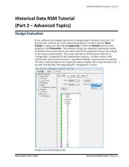
To review the alias structure, click on the design Evaluation node and for Order select
2FI (two-factor interaction) and click on Results. In the table below, we ignored
interactions of three or more factors, and underlined the two-factor interactions of
interest.
Factorial Effects Aliases
[Est. Terms] Aliased Terms
[Intercept] = Intercept
[A] = A - EF - GH
[B] = B - EG - FH
[C] = C - HJ
[D] = D - EJ
[E] = E - AF - BG - DJ
[F] = F - AE - BH
[G] = G - AH - BE
[H] = H - AG - BF - CJ
[J] = J - CH - DE
[AB] = AB + CD + EH + FG
[AC] = AC + BD + GJ
[AD] = AD + BC + FJ
[AJ] = AJ + CG + DF
[BJ] = BJ + CF + DG
[CE] = CE + DH
Alias structure after deleting columns from L16
Notice that all of the main effects, plus the four interactions of interest, are aliased with
one or more two-factor interactions. The effects now labeled BJ and CE are the two
columns used to estimate error, but they too are aliased with two-factor interactions. All
of these aliased interactions must be negligible for an accurate analysis.
Design-Expert 7 User’s Guide Taguchi Design Tutorial • 7

Analyze the Results
To analyze the results, follow the usual procedure for two-level factorials as illustrated
earlier in the Factorial Design Tutorials. (If you haven’t already done so, go back and
complete this tutorial.)
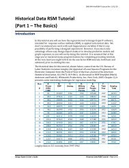
Click on the analysis node labeled Tensile, which is found in the tree structure along
the left of the main window. Then, click on the Effects button displayed in the toolbar
at the top of the main window. Click on the two largest effects (J and D) on the halfnormal
plot of effects, or lasso them as shown.
Half normal plot of effects
On the Effects Tool press the Pareto Chart for another view on the relative
magnitude of effects. It’s very clear now that factors J and D stand out.
Pareto chart of effects
8 • Taguchi DesignTutorial Design-Expert 7 User’s Guide

DX7-03E-Taguchi.doc Rev. 4/10/06
Click on the ANOVA button. Design-Expert now warns you about aliasing and offers a
list for you to view.
Warning that design contains aliased terms
Click Yes to see the aliases again – this time with modeled terms identified by “M” and
the others labeled “e” for error.
View of alias list
Again, click on the ANOVA button. You should now see an annotated ANOVA report
by default. If not, select View, Annotated ANOVA. The ANOVA confirms that the
effects of D and J are statistically significant.
Design-Expert 7 User’s Guide Taguchi Design Tutorial • 9

ANOVA report
Click on the Diagnostics button. The graphs don’t look great, but they’re acceptable.
Click on the Model Graphs button. A graph of factor D (drying) should now appear.
One-factor plot of the main effect of factor D (drying)
You may be wondering about the circular symbols. As indicated by the legend, these
are actual design points. Due to the fractional nature of Taguchi designs, you won’t see
too many points on the plots of predicted effects. Click on those points that do appear to
get a readout of their actual response value.
10 • Taguchi DesignTutorial Design-Expert 7 User’s Guide

DX7-03E-Taguchi.doc Rev. 4/10/06
On the Factors Tool, click the Term down arrow and select J (or right-click on the J
bar to make it the X1-axis). Notice that Design-Expert defaults to the “lower” level of
the categorical factors.
Plotting the second significant main effect (J)
Click on the upper point of the D:Drying, which we now know is best for tensile
strength.
Plot of main effect J (material) with factor D set at high level
The square symbols at either end of the lines show the predicted outcomes. The bars
going up and down from these points represent the least significant difference (LSD) at a
95% confidence level (the default). Click on the predicted value at the upper left to get a
readout on the LSD (printed to the left of the graph). Note that this LSD does not
overlap with the one at the lower right. This provides visual verification that the effect
shown on the plot is statistically significant.
Design-Expert 7 User’s Guide Taguchi Design Tutorial • 11

Maximal point clicked with predicted response noted and LSD reported
This concludes our tutorial on Taguchi orthogonal arrays. Use these designs with
caution! Take advantage of Design-Expert’s design evaluation feature for examining
aliases. Make sure that likely interactions are not confounded with main effects. For
example, in this case, only two main effects (D and J) appear to be significant, but as
shown in the alias table, perhaps D is really EJ, and J could be CH and/or DE.
Therefore, it would be a good idea to do a followup experiment to confirm the effects of
D and J.
12 • Taguchi DesignTutorial Design-Expert 7 User’s Guide