Non-neutral plasma equilibria with weak axisymmetric magnetic ...

092108-2 Kotelnikov, Romé, and Kabantsev Phys. Plasmas 13, 092108 2006
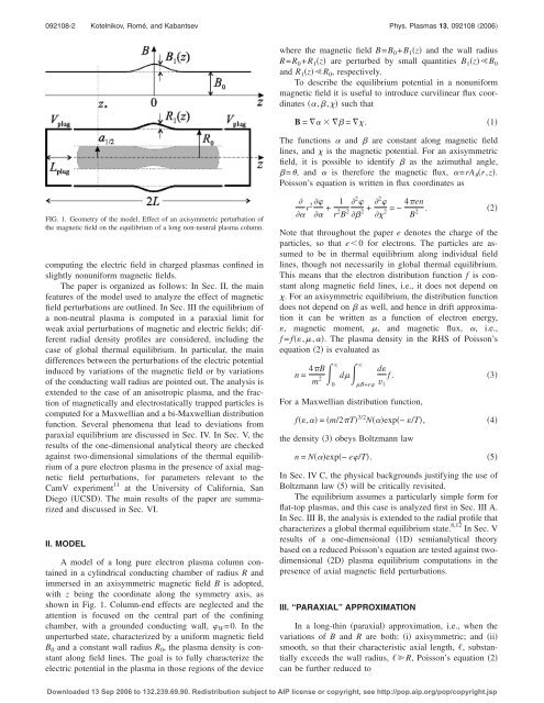
where the magnetic field B=B 0 +B 1 z and the wall radius
R=R 0 +R 1 z are perturbed by small quantities B 1 zB 0
and R 1 zR 0 , respectively.
To describe the equilibrium potential in a nonuniform
magnetic field it is useful to introduce curvilinear flux coordinates
,, such that
B = = .
1
The functions and are constant along magnetic field
lines, and is the magnetic potential. For an axisymmetric
field, it is possible to identify as the azimuthal angle,
=, and is therefore the magnetic flux, =rA r,z.
Poisson’s equation is written in flux coordinates as
FIG. 1. Geometry of the model. Effect of an axisymmetric perturbation of
the magnetic field on the equilibrium of a long non-neutral plasma column.
computing the electric field in charged plasmas confined in
slightly nonuniform magnetic fields.
The paper is organized as follows: In Sec. II, the main
features of the model used to analyze the effect of magnetic
field perturbations are outlined. In Sec. III the equilibrium of
a non-neutral plasma is computed in a paraxial limit for
weak axial perturbations of magnetic and electric fields; different
radial density profiles are considered, including the
case of global thermal equilibrium. In particular, the main
differences between the perturbations of the electric potential
induced by variations of the magnetic field or by variations
of the conducting wall radius are pointed out. The analysis is
extended to the case of an anisotropic plasma, and the fraction
of magnetically and electrostatically trapped particles is
computed for a Maxwellian and a bi-Maxwellian distribution
function. Several phenomena that lead to deviations from
paraxial equilibrium are discussed in Sec. IV. In Sec. V, the
results of the one-dimensional analytical theory are checked
against two-dimensional simulations of the thermal equilibrium
of a pure electron plasma in the presence of axial magnetic
field perturbations, for parameters relevant to the
CamV experiment 11 at the University of California, San
Diego UCSD. The main results of the paper are summarized
and discussed in Sec. VI.
II. MODEL
A model of a long pure electron plasma column contained
in a cylindrical conducting chamber of radius R and
immersed in an axisymmetric magnetic field B is adopted,
with z being the coordinate along the symmetry axis, as
shown in Fig. 1. Column-end effects are neglected and the
attention is focused on the central part of the confining
chamber, with a grounded conducting wall, W =0.Inthe
unperturbed state, characterized by a uniform magnetic field
B 0 and a constant wall radius R 0 , the plasma density is constant
along field lines. The goal is to fully characterize the
electric potential in the plasma in those regions of the device
r2 + 1
r 2 B 2 2
2 + 2
2 =−4en B 2 . 2
Note that throughout the paper e denotes the charge of the
particles, so that e0 for electrons. The particles are assumed
to be in thermal equilibrium along individual field
lines, though not necessarily in global thermal equilibrium.
This means that the electron distribution function f is constant
along magnetic field lines, i.e., it does not depend on
. For an axisymmetric equilibrium, the distribution function
does not depend on as well, and hence in drift approximation
it can be written as a function of electron energy,
, magnetic moment, , and magnetic flux, , i.e.,
f = f,,. The plasma density in the RHS of Poisson’s
equation 2 is evaluated as
n = 4B
m 2 0
dB+e
d
v
f .
For a Maxwellian distribution function,
f, = m/2T 3/2 Nexp− /T,
the density 3 obeys Boltzmann law
n = Nexp− e/T.
In Sec. IV C, the physical backgrounds justifying the use of
Boltzmann law 5 will be critically revisited.
The equilibrium assumes a particularly simple form for
flat-top plasmas, and this case is analyzed first in Sec. III A.
In Sec. III B, the analysis is extended to the radial profile that
characterizes a global thermal equilibrium state. 8,12 In Sec. V
results of a one-dimensional 1D semianalytical theory
based on a reduced Poisson’s equation are tested against twodimensional
2D plasma equilibrium computations in the
presence of axial magnetic field perturbations.
III. “PARAXIAL” APPROXIMATION
In a long-thin paraxial approximation, i.e., when the
variations of B and R are both: i axisymmetric; and ii
smooth, so that their characteristic axial length, , substantially
exceeds the wall radius, R, Poisson’s equation 2
can be further reduced to
3
4
5
Downloaded 13 Sep 2006 to 132.239.69.90. Redistribution subject to AIP license or copyright, see http://pop.aip.org/pop/copyright.jsp