An equipment and software for improved estimation of soil acidity
An equipment and software for improved estimation of soil acidity
An equipment and software for improved estimation of soil acidity

You also want an ePaper? Increase the reach of your titles
YUMPU automatically turns print PDFs into web optimized ePapers that Google loves.
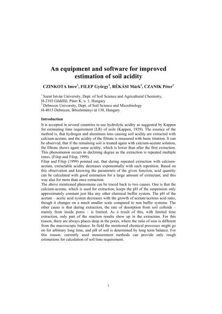
<strong>An</strong> <strong>equipment</strong> <strong>and</strong> <strong>s<strong>of</strong>tware</strong> <strong>for</strong> <strong>improved</strong><br />
<strong>estimation</strong> <strong>of</strong> <strong>soil</strong> <strong>acidity</strong><br />
CZINKOTA Imre 1 , FILEP György 2 , RÉKÁSI Márk 2 , CZANIK Péter 1<br />
1<br />
Szent István University, Dept. <strong>of</strong> Soil Science <strong>and</strong> Agricultural Chemistry,<br />
H-2103 Gödöllő, Páter K. u. 1, Hungary<br />
2<br />
Debrecen University, Dept. <strong>of</strong> Soil Science <strong>and</strong> Microbiology<br />
H-4015 Debrecen, Böszörményi út 138, Hungary<br />
Introduction<br />
It is accepted in several countries to use hydrolytic <strong>acidity</strong> as suggested by Kappen<br />
<strong>for</strong> estimating lime requirement (LR) <strong>of</strong> <strong>soil</strong>s (Kappen, 1929). The essence <strong>of</strong> the<br />
method is, that hydrogen <strong>and</strong> aluminum ions causing <strong>soil</strong> <strong>acidity</strong> are extracted with<br />
calcium-acetate, <strong>and</strong> the <strong>acidity</strong> <strong>of</strong> the filtrate is measured with basic titration. It can<br />
be observed, that if the remaining <strong>soil</strong> is treated again with calcium-acetate solution,<br />
the filtrate shows again some <strong>acidity</strong>, which is lower than after the first extraction.<br />
This phenomenon occurs in declining degree as the extraction is repeated multiple<br />
times. (Filep <strong>and</strong> Filep, 1999).<br />
Filep <strong>and</strong> Filep (1999) pointed out, that during repeated extraction with calciumacetate,<br />
extractable <strong>acidity</strong> decreases exponentially with each repetition. Based on<br />
this observation <strong>and</strong> knowing the parameters <strong>of</strong> the given function, acid quantity<br />
can be calculated with good <strong>estimation</strong> <strong>for</strong> a large amount <strong>of</strong> extractant, <strong>and</strong> this<br />
way also <strong>for</strong> more than once extraction.<br />
The above mentioned phenomena can be traced back to two causes. One is that the<br />
calcium-acetate, which is used <strong>for</strong> extraction, keeps the pH <strong>of</strong> the suspension only<br />
approximately constant just like any other chemical buffer system. The pH <strong>of</strong> the<br />
acetate – acetic acid system decreases with the growth <strong>of</strong> acetate/acetous acid ratio,<br />
though it changes on a much smaller scale compared to non buffer systems. The<br />
other cause is that during extraction, the rate <strong>of</strong> desorption from <strong>soil</strong> colloids –<br />
mainly from inside pores – is limited. As a result <strong>of</strong> this, with limited time<br />
extraction, only part <strong>of</strong> the reaction results show up in the extractum. For this<br />
reason, there are always places deep in the pores, where the ratio <strong>of</strong> ions is different<br />
from the macroscopic balance. In field the mentioned chemical processes might go<br />
on <strong>for</strong> arbitrary long time, <strong>and</strong> pH <strong>of</strong> <strong>soil</strong> is determined by long term balance. For<br />
this reason, currently used measurement methods can provide only rough<br />
<strong>estimation</strong>s <strong>for</strong> calculation <strong>of</strong> <strong>soil</strong> lime requirement.<br />
1
In accordance with the previous paragraphs, the measurement method to determine<br />
punctual potential <strong>acidity</strong> should have the following characteristics: it can be kept at<br />
an exact pH value, it can follow a process <strong>for</strong> arbitrary long time, <strong>and</strong> it is exact<br />
enough to allow reliable extrapolation <strong>of</strong> data to infinite time. It is quite difficult<br />
<strong>and</strong> complicated to fulfill these requirements with a purely chemical system, so we<br />
have built a combined, computer controlled measurement system to solve the<br />
problem.<br />
Materials <strong>and</strong> methods<br />
Enhanced determination <strong>of</strong> hydrolytic <strong>acidity</strong> is based on the following theory:<br />
During the desorption <strong>of</strong> ions causing <strong>acidity</strong>, pH is repeatedly measured in<br />
negligible intervals compared to the full time <strong>of</strong> examination. When it is lower than<br />
a given value, base is fed, so the system is artificially buffered. In a st<strong>and</strong>-alone<br />
system, pH is continuously decreasing due to continuous movement <strong>of</strong> H + <strong>and</strong> Al 3+<br />
ions into the solution, so an outer intervention to increase pH is sufficient. Since<br />
solid <strong>and</strong> liquid stages are not separated during the use <strong>of</strong> this measurement method,<br />
<strong>and</strong> there is no intervention to cause a sudden change in the system, the reaction can<br />
be continued <strong>for</strong> arbitrary time. To evaluate results, it is enough to note time <strong>and</strong><br />
added quantities, <strong>and</strong> to extrapolate to infinite time using a function fitted on this<br />
data. Lengthening the time <strong>of</strong> measurement can <strong>of</strong> course decrease the error <strong>of</strong><br />
extrapolation, so it is practical to apply longer measurement times <strong>for</strong> more exact<br />
results.<br />
Equipment to put the given theory in practice<br />
The pH <strong>of</strong> <strong>soil</strong> suspension, which is continuously stirred with a proper speed, is<br />
continuously measured with a pH-selective electrode. The <strong>soil</strong> suspension is<br />
prepared with KCl solution, as the noise <strong>of</strong> pH-electrode is considerably higher<br />
when distilled water is used to prepare the <strong>soil</strong> suspension. With a relatively<br />
concentrated KCl solution, ionic strength can be kept at a relatively constant value.<br />
Signals from the pH electrode are first amplified then digitized to provide input <strong>for</strong><br />
the computer, where they are trans<strong>for</strong>med to pH values using preliminary<br />
calibration. <strong>An</strong> outline <strong>of</strong> the <strong>equipment</strong> can be seen on Figure 1.<br />
The <strong>s<strong>of</strong>tware</strong> on the computer compares the incoming pH values in predefined time<br />
intervals with a predefined pH limit value. If the measured pH value is lower than<br />
the limit pH value, the computer sends a signal to an automatic burette, which adds<br />
to the <strong>soil</strong> suspension the smallest amount <strong>of</strong> basic solution possible to add by the<br />
burette. This method helps to keep the pH value <strong>of</strong> the system close to a predefined<br />
2
value, with the best precision possible. After each lapse <strong>of</strong> the time interval the<br />
<strong>s<strong>of</strong>tware</strong> saves the time, pH <strong>and</strong> added quantity data on the disk. Saved data are<br />
evaluated automatically using nonlinear regression analysis, when a predefined<br />
measurement time is over, or when the measurement process is stopped by the<br />
experimenter. Figure 2. shows the theoretical outline <strong>of</strong> the <strong>s<strong>of</strong>tware</strong>. The<br />
measurement system was built using Radelkis OP-0808P pH electrode, Schott<br />
Titronic 96 automatic burette, ALTAIR BT AAD2816S amplifier <strong>and</strong> analog digital<br />
converter <strong>and</strong> an I486 personal computer.<br />
Properties <strong>of</strong> the examined <strong>soil</strong>s are shown in Table 1.<br />
4g <strong>of</strong> <strong>soil</strong> sample was suspended in 160 cm 3 <strong>of</strong> 0.1 M KCl solution. 0.1 M NaOH<br />
solution was used <strong>for</strong> titration. The limit value was pH 8.2 <strong>and</strong> the time interval<br />
between measurements was 10 sec. Maximum time <strong>of</strong> measurements was 12 hours.<br />
Results <strong>and</strong> discussion<br />
On Figure 3. data from sample 1. can be seen, pH values <strong>and</strong> volume <strong>of</strong> fed basic<br />
solution in function <strong>of</strong> time.<br />
The figure shows that at the given resolution, pH value can be considered as<br />
constant after an initial rising phase. The almost linear rise <strong>of</strong> pH at the beginning<br />
<strong>of</strong> measurements is to be interpreted in the following way: H + <strong>and</strong> Al 3+ ions already<br />
in the solution or desorbing instantly, react to the fed base solution immediately, so<br />
in this linear phase base solution is fed in each cycle <strong>of</strong> measurement evaluation. In<br />
effect, steepness <strong>of</strong> the rising pH curve is characterized by feeding speed,<br />
determined by cycles <strong>of</strong> the <strong>equipment</strong>. For this reason, this part cannot be used to<br />
kinetically analyze the curve, as it increases the error <strong>of</strong> measurement. There<strong>for</strong>e,<br />
this part <strong>of</strong> the data is omitted during evaluation.<br />
However, looking at the pH curve at a better resolution (Figure 4.) the essence <strong>of</strong><br />
the examination can be seen. This is that when base solution is added, pH value<br />
rises sharply (even if this rise is quite small), then it decreases under the<br />
predetermined pH limit more <strong>and</strong> more slowly with lapse <strong>of</strong> time <strong>and</strong> increase <strong>of</strong><br />
added base solution.<br />
It can be seen on Figure 3. that the volume <strong>of</strong> added base solution grows almost like<br />
an exponential associate function. Because <strong>of</strong> the sudden change <strong>of</strong> rise in the first<br />
section, we adopt the mathematical description <strong>of</strong> Filep <strong>and</strong> Csubák (1997) to<br />
define this growth. This description is a first order kinetic equation, which was<br />
fitted with two different speed constants: one faster, belonging supposedly to ions<br />
in the solution <strong>and</strong> quickly desorbable ions from the outer surface, <strong>and</strong> one slower,<br />
belonging supposedly to ions desorbed in the inner pores. The applied <strong>for</strong>mula has<br />
the following <strong>for</strong>m:<br />
3
−c1t<br />
−c2t<br />
y = A ⋅( 1−<br />
e ) + A ⋅(1<br />
− e )<br />
1<br />
y amount <strong>of</strong> fed base, cm 3<br />
t time, sec<br />
A 1 base consumption <strong>of</strong> faster process, cm 3<br />
A 2 base consumption <strong>of</strong> slower process, cm 3<br />
k 1 rate constant <strong>of</strong> faster process, s -1<br />
k 2 rate constant <strong>of</strong> slower process, s -1<br />
2<br />
The curve fitted on the data is shown on Figure 5. It can be seen on this figure that<br />
measured values are approximately equal to the fitted function’s graph.<br />
It can be seen on Table 2. that the error <strong>of</strong> fitting is around 0.3 %. There<strong>for</strong>e these<br />
processes can be estimated very accurately with the use <strong>of</strong> measurement data.<br />
Measurement results after two hours (7200 sec) <strong>of</strong> reaction time account near half<br />
<strong>of</strong> the full <strong>acidity</strong>. This corresponds mainly to the fast process (1.6 cm 3 /sample 1/).<br />
The rest (3.05 cm 3 /sample 1/) is available only with a multiple day measurement or<br />
curve fitting (Figure 6.).<br />
Full <strong>acidity</strong>, <strong>and</strong> on its basis lime requirement (CaCO 3 g.kg <strong>soil</strong> -1 ) is to be calculated<br />
with the two base consumption parameters using the following <strong>for</strong>mula:<br />
LR =<br />
( A + A )<br />
1<br />
2<br />
⋅c<br />
2⋅<br />
m<br />
<strong>soil</strong><br />
base<br />
⋅c<br />
LR<br />
-1<br />
Lime Requirement, g.kg <strong>soil</strong><br />
m <strong>soil</strong> Amount <strong>of</strong> examined <strong>soil</strong>, g<br />
c base Concentration <strong>of</strong> NaOH solution, mol.dm -3<br />
c l CaCO 3 content, % <strong>of</strong> lime.<br />
l<br />
In Table 3. the lime requirement calculated by the new method is compared with<br />
that calculated by the method <strong>of</strong> Kappen. It can be seen that the lime amounts<br />
calculated with the new <strong>for</strong>mula are considerabely different from those calculated<br />
with the method <strong>of</strong> Kappen.<br />
Conclusions<br />
We built a measurement <strong>equipment</strong> to eliminate problems <strong>of</strong> such balance systems<br />
that are created with chemical extractants effective <strong>for</strong> a limited time. The<br />
measurement is fully automated, requires no manual intervention with the exception<br />
4
<strong>of</strong> sample preparation, <strong>and</strong> might last <strong>for</strong> arbitrary time. To increase the efficiency<br />
<strong>of</strong> measurement method, it is possible to collect measurement data from multiple<br />
sources <strong>and</strong> control multiple burettes with one data collecting / controlling<br />
computer. Precision <strong>of</strong> calculated results is very good, the error is about 0.3 %. This<br />
is due to the large amount <strong>of</strong> data obtained with frequent measurement cycles, <strong>and</strong><br />
evaluation <strong>of</strong> data with nonlinear fitting. When pH is kept at a constant value,<br />
movement <strong>of</strong> adsorbed H + <strong>and</strong> Al 3+ ions into the solution can be satisfyingly<br />
modeled as the addition <strong>of</strong> two first order kinetic equation, where a quick process<br />
taking place <strong>for</strong> one-two hours <strong>and</strong> a slow process taking place probably <strong>for</strong> days<br />
can be distinguished.<br />
The measurement theory <strong>and</strong> <strong>equipment</strong> elaborated are suitable to kinetically<br />
examine any process <strong>of</strong> sorption or ion exchange taking place on surface <strong>of</strong> <strong>soil</strong><br />
colloids, if one condition is fulfilled. This condition is, that the examined matter or<br />
parameter to measure can be somehow trans<strong>for</strong>med into electric signals without<br />
changing the system. For example, long-term exchange <strong>of</strong> polluting or nutritive<br />
materials can be measured with ion selective electrodes, or redox properties <strong>of</strong> <strong>soil</strong>s<br />
can be measured with platinum electrodes.<br />
References<br />
Filep, Gy. <strong>and</strong> Csubák, M. 1997.: Kinetics <strong>of</strong> surface reactions involving proton transfer in<br />
<strong>soil</strong>/aqueous solution systems. (in Hung.) Agrokémia és Talajtan No. 1-4. pp.159-170.<br />
Filep, Gy. <strong>and</strong> Filep, T. 1999.: Characterization <strong>of</strong> <strong>for</strong>ms potential <strong>soil</strong> <strong>acidity</strong>. (in Hung.)<br />
Agrokémia és Talajtan No. 1-2. pp. 33-48.<br />
Kappen, H., 1929. Die Bodenazidität. Springer Verlag. Berlin.<br />
5
Summary<br />
In some countries it is accepted <strong>for</strong> estimating the lime requirement (LR) to use<br />
hydrolytic <strong>acidity</strong> suggested by Kappen, which is based on a single time extraction<br />
<strong>of</strong> hydrogen- <strong>and</strong> aluminum-ion with calcium-acetate. We could achieve more<br />
accurate results, if we measure the total surface <strong>acidity</strong> (TSA) <strong>of</strong> <strong>soil</strong>s. For this<br />
reason it is an improvement to use a direct measurement method <strong>and</strong> <strong>equipment</strong>,<br />
which is suitable to estimate the results <strong>of</strong> long-term processes <strong>and</strong> TSA, via<br />
investigating the kinetic properties <strong>of</strong> desorption.<br />
The method <strong>of</strong> measurement: A pH electrode is dipped into continuously stirred <strong>soil</strong><br />
suspension, containing background salt (e.g. KCl), <strong>and</strong> it is connected to a computer<br />
using an amplifier <strong>and</strong> A/D converter. A computer program has been developed that<br />
controls an automatic burette, which adds the base solution into the system if pH is<br />
less than the pre-adjusted value (e.g. pH 6.5 or pH 6.8) <strong>and</strong> stops adding if pH<br />
reaches this value.<br />
For evaluation, the amount <strong>of</strong> added base vs. time data series can be used. With<br />
increasing time the amount <strong>of</strong> added base keeps to a constant (asymptotic) value.<br />
The program fits an exponential associate function on measured data, <strong>and</strong> outputs<br />
the asymptotic value connecting to infinite time, which can be used to calculate LR.<br />
Let us suppose that there are two processes with different rate, in this case the<br />
function can be created as the addition <strong>of</strong> two first order kinetic sub-processes.<br />
−c1t<br />
−c2t<br />
y = b1<br />
⋅ ( 1−<br />
e ) + b2<br />
⋅ (1 − e )<br />
The faster process that takes place on the outer surfaces features easily removable<br />
<strong>acidity</strong>, <strong>and</strong> the slower process probably describes processes inside the deeper<br />
pores. The fitting error <strong>of</strong> parameters is about 0.3 %, which means, that the TSA<br />
value, based on these measured data <strong>and</strong> method can be estimated with high<br />
accuracy.<br />
The measurement is fully automated. The evaluation is based on extrapolation so<br />
the precision <strong>of</strong> results increases with the number <strong>of</strong> measurement points <strong>and</strong> the<br />
length <strong>of</strong> measurement time. Depending on the application, a quick measurement<br />
with approximate results or a longer measurement with more precise results can be<br />
chosen.<br />
6
Stirrer<br />
Elektrode voltage (analog signal) pH electrode Soil suspension<br />
Amplifyer &<br />
AD converter<br />
Elektrode voltage (digital signal)<br />
Reagent solution<br />
Computer<br />
Automatic<br />
burette<br />
Burette control (digital signal)<br />
Feeded volume (digital signal)<br />
Figure 1. Theoretical outline <strong>of</strong> the <strong>equipment</strong><br />
Start<br />
Calibrate<br />
No<br />
Yes<br />
Measurement<br />
Measurement<br />
No<br />
St<strong>and</strong>ard1 <br />
Yes<br />
No<br />
Timer<br />
Yes<br />
Ask st<strong>and</strong>ard2<br />
Ask st<strong>and</strong>ard1<br />
No<br />
End <strong>of</strong> meas.<br />
Yes<br />
Meas. voltage<br />
Meas. voltage Meas. voltage<br />
No<br />
The other st<strong>and</strong>ard OK<br />
Yes<br />
Calculating pH-voltage function<br />
Save caibration data<br />
Store all data<br />
Close files<br />
Fitting function<br />
Output parameters<br />
End<br />
Feed one step<br />
Calculating pH<br />
No<br />
Yes pH
Figure 3. Graphical display <strong>of</strong> data saved during measurement (Sample 1)<br />
Figure 4. Magnified view <strong>of</strong> a part <strong>of</strong> the measured curves (Sample 1)<br />
8
5,0<br />
4,5<br />
4,0<br />
3<br />
Added NaOH, cm<br />
3,5<br />
3,0<br />
2,5<br />
2,0<br />
1,5<br />
1,0<br />
0,5<br />
0,0<br />
Measured value<br />
Calculated value<br />
0 5000 10000 15000 20000 25000 30000<br />
Time, sec<br />
Figure 5. Graph <strong>of</strong> the fitted function (Sample 1)<br />
9
5,0 A<br />
4,5<br />
Asymptotic value<br />
4,0<br />
3,5<br />
2 hours<br />
Added NaOH, cm 3<br />
3,0<br />
2,5<br />
2,0<br />
1,5<br />
1,0<br />
0,5<br />
Total kinetic process<br />
Faster kinetic process<br />
Slower kinetic process<br />
Measured value<br />
0,0<br />
0 5000 10000 15000 20000 25000 30000<br />
Time, sec<br />
B<br />
2,0<br />
Asymptotic value<br />
Added NaOH, cm 3<br />
1,5<br />
1,0<br />
0,5<br />
2 hours<br />
Total kinetic process<br />
Faster kinetic process<br />
Slower kinetic process<br />
Measured value<br />
0,0<br />
0 5000 10000 15000 20000 25000 30000 35000 40000<br />
Time, sec<br />
Figure 6. The two parts <strong>of</strong> the fitted function. A: Sample 1; B: Sample 3<br />
10
N o <strong>of</strong> sample pH (KCl) OM% Clay+Silt*%<br />
1 4.7 1.2 39.7<br />
2 4,0 1,9 69,0<br />
3 3,7 0,9 11,0<br />
4 4,1 1,1 20,1<br />
5 4,2 3,1 68,0<br />
*Clay+Silt% < 0.02 mm<br />
Table 1. Some properties <strong>of</strong> the examined <strong>soil</strong>s<br />
N o <strong>of</strong> sample Parameter Value Error Error %<br />
A 1 cm 3 1.6054 0.007 0.43<br />
1 k 1 s -1 0.00336 0.00004 1.19<br />
A 2 cm 3 3.0572 0.0105 0.34<br />
k 2 s -1 0.00008 8.41 10 -7 1.05<br />
R 2 0.9976<br />
A 1 cm 3 2.25674 0.00435 0.19<br />
2 k 1 s -1 0.00167 6.6182 10 -6 0.39<br />
A 2 cm 3 1.63498 0.00385 0.23<br />
k 2 s -1 0.0001 8.3434 10 -7 0.83<br />
R 2 0.9988<br />
A 1 cm 3 0.63475 0.00195 0.30<br />
3 k 1 s -1 0.00536 0.00007 1.30<br />
A 2 cm 3 1.61516 0.00668 0.41<br />
k 2 s -1 0.00005 4.4444 10 -7 0.88<br />
R 2 0.9986<br />
A 1 cm 3 1.13408 0.00362 0.31<br />
4 k 1 s -1 0.00313 0.00003 0.95<br />
A 2 cm 3 1.27671 0.00601 0.47<br />
k 2 s -1 0.00007 1.0355 10 -6 1.47<br />
R 2 0.9971<br />
A 1 cm 3 1.88475 0.00652 0.34<br />
5 k 1 s -1 0.00196 0.00002 1.02<br />
A 2 cm 3 1.3581 0.00662 0.48<br />
k 2 s -1 0.00008 1.5049 10 -6 1.88<br />
R 2 0.9951<br />
Table 2. Parameter values <strong>of</strong> curve fitting<br />
11
N o <strong>of</strong> sample LR 1 LR 2<br />
1 5.82 3.65<br />
2 4.86 5.27<br />
3 2.81 3.70<br />
4 3.01 4.96<br />
5 4.05 6.51<br />
Table 3. The lime requirement calculated with the two different methods<br />
LR1: The lime requirement calculated with the new <strong>for</strong>mula<br />
LR2: The lime requirement calculated with the method <strong>of</strong> Kappen<br />
12