Statistical thermodynamics 1: the concepts - W.H. Freeman

More documents

Recommendations

Info

$Microscopy Math - W.H. Freeman$

PC8eC16 1/27/06 22:03 Page 565 16.2 THE MOLECULAR PARTITION FUNCTION 565 this expression applies only to unsymmetrical linear rotors (for instance, HCl, not CO 2 ). Self-test 16.2 Write the partition function for a two-level system, the lower state (at energy 0) being nondegenerate, and the upper state (at an energy ε) doubly degenerate. [q = 1 + 2e −βε ] e (a) An interpretation of the partition function Some insight into the significance of a partition function can be obtained by considering how q depends on the temperature. When T is close to zero, the parameter β = 1/kT is close to infinity. Then every term except one in the sum defining q is zero because each one has the form e −x with x →∞. The exception is the term with ε 0 ≡ 0 (or the g 0 terms at zero energy if the ground state is g 0 -fold degenerate), because then ε 0 /kT ≡ 0 whatever the temperature, including zero. As there is only one surviving term when T = 0, and its value is g 0 , it follows that lim q = g 0 (16.10) T→0 That is, at T = 0, the partition function is equal to the degeneracy of the ground state. Now consider the case when T is so high that for each term in the sum ε j /kT ≈ 0. Because e −x = 1 when x = 0, each term in the sum now contributes 1. It follows that the sum is equal to the number of molecular states, which in general is infinite: lim q =∞ (16.11) T→∞ In some idealized cases, the molecule may have only a finite number of states; then the upper limit of q is equal to the number of states. For example, if we were considering only the spin energy levels of a radical in a magnetic field, then there would be only two states (m s =± – 1 2 ). The partition function for such a system can therefore be expected to rise towards 2 as T is increased towards infinity. We see that the molecular partition function gives an indication of the number of states that are thermally accessible to a molecule at the temperature of the system. At T = 0, only the ground level is accessible and q = g 0 . At very high temperatures, virtually all states are accessible, and q is correspondingly large. Example 16.2 Evaluating the partition function for a uniform ladder of energy levels Evaluate the partition function for a molecule with an infinite number of equally spaced nondegenerate energy levels (Fig. 16.3). These levels can be thought of as the vibrational energy levels of a diatomic molecule in the harmonic approximation. Method We expect the partition function to increase from 1 at T = 0 and approach infinity as T to ∞. To evaluate eqn 16.8 explicitly, note that 1 1 + x + x 2 + ···= 1 − x Answer If the separation of neighbouring levels is ε, the partition function is 1 q = 1 + e −βε + e −2βε + ···= 1 + e −βε + (e −βε ) 2 + ···= 1 − e −βε This expression is plotted in Fig. 16.4: notice that, as anticipated, q rises from 1 to infinity as the temperature is raised. 3e 2e e 0 Fig. 16.3 The equally spaced infinite array of energy levels used in the calculation of the partition function. A harmonic oscillator has the same spectrum of levels. Comment 16.3 The sum of the infinite series S = 1 + x + x 2 + · · · is obtained by multiplying both sides by x, which gives xS = x + x 2 + x 3 + · · · = S − 1 and hence S = 1/(1 − x). 10 q 5 0 0 5 10 kT/ Fig. 16.4 The partition function for the system shown in Fig.16.3 (a harmonic oscillator) as a function of temperature. Exploration Plot the partition function of a harmonic oscillator against temperature for several values of the energy separation ε. How does q vary with temperature when T is high, in the sense that kT >> ε (or βε
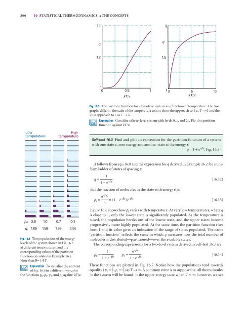
PC8eC16 1/26/06 14:34 Page 566 566 16 STATISTICAL THERMODYNAMICS 1: THE CONCEPTS 1.4 2 q q 1.2 1.5 1 0 0.5 1 kT/ 1 0 5 10 kT/ Low temperature High temperature Fig. 16.5 The partition function for a two-level system as a function of temperature. The two graphs differ in the scale of the temperature axis to show the approach to 1 as T → 0 and the slow approach to 2 as T →∞. Exploration Consider a three-level system with levels 0, ε, and 2ε. Plot the partition function against kT/ε. Self-test 16.3 Find and plot an expression for the partition function of a system with one state at zero energy and another state at the energy ε. [q = 1 + e −βε , Fig. 16.5] It follows from eqn 16.8 and the expression for q derived in Example 16.2 for a uniform ladder of states of spacing ε, 1 q = (16.12) 1 − e −βε that the fraction of molecules in the state with energy ε i is 3.0 1.0 0.7 0.3 q: 1.05 1.58 1.99 3.86 Fig. 16.6 The populations of the energy levels of the system shown in Fig.16.3 at different temperatures, and the corresponding values of the partition function calculated in Example 16.2. Note that β = 1/kT. Exploration To visualize the content of Fig. 16.6 in a different way, plot the functions p 0 , p 1 , p 2 , and p 3 against kT/ε. e −βε i p i = =(1 − e −βε )e −βε i (16.13) q Figure 16.6 shows how p i varies with temperature. At very low temperatures, where q is close to 1, only the lowest state is significantly populated. As the temperature is raised, the population breaks out of the lowest state, and the upper states become progressively more highly populated. At the same time, the partition function rises from 1 and its value gives an indication of the range of states populated. The name ‘partition function’ reflects the sense in which q measures how the total number of molecules is distributed—partitioned—over the available states. The corresponding expressions for a two-level system derived in Self-test 16.3 are 1 e −βε p 0 = p 1 = (16.14) 1 + e −βε 1 + e −βε These functions are plotted in Fig. 16.7. Notice how the populations tend towards equality (p 0 = – 1 2 , p 1 = – 1 2 ) as T →∞. A common error is to suppose that all the molecules in the system will be found in the upper energy state when T =∞; however, we see
Page 1 and 2: PC8eC16 1/26/06 14:34 Page 560 16 S
Page 3 and 4: PC8eC16 1/26/06 14:34 Page 562 562
Page 5: PC8eC16 1/26/06 14:34 Page 564 564
Page 29: PC8eC16 1/26/06 14:34 Page 588 588

Statistical thermodynamics 1: the concepts - W.H. Freeman

Create successful ePaper yourself

Delete template?

Save as template?