GLI Atmosphere Brochure (PDF file)
GLI Atmosphere Brochure (PDF file)
GLI Atmosphere Brochure (PDF file)

Create successful ePaper yourself
Turn your PDF publications into a flip-book with our unique Google optimized e-Paper software.
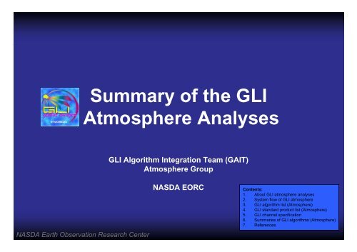
Summary of the <strong>GLI</strong><br />
<strong>Atmosphere</strong> Analyses<br />
<strong>GLI</strong> Algorithm Integration Team (GAIT)<br />
<strong>Atmosphere</strong> Group<br />
NASDA Earth Observation Research Center<br />
NASDA EORC<br />
Contents:<br />
1. About <strong>GLI</strong> atmosphere analyses<br />
2. System flow of <strong>GLI</strong> atmosphere<br />
3. <strong>GLI</strong> algorithm list (<strong>Atmosphere</strong>)<br />
4. <strong>GLI</strong> standard product list (<strong>Atmosphere</strong>)<br />
5. <strong>GLI</strong> channel specification<br />
6. Summaries of <strong>GLI</strong> algorithms (<strong>Atmosphere</strong>)<br />
7. References
Abuot <strong>GLI</strong> atmosphere analyses<br />
Cloud, aerosol, and water vapor parameters<br />
Our inability to adequately model cloud processes is a major obstacle in accurate simulations of global warming<br />
scenarios. Low-level clouds and upper-level clouds play different roles in the climate system. How they change<br />
through the global warming process is, at present, not fully understood. Aerosols are also important for the<br />
global warming issue, as revealed by several recent studies on direct aerosol and indirect cloud-aerosol<br />
interaction effects on the Earth's climate. It is, therefore, important to generate global archives of geophysical<br />
parameters related to cloud, aerosol, and water vapor fields. Using these data sets, we should study the global<br />
distribution, annual variability, and feedback mechanisms of the climate field.<br />
*Water vapor algorithms and products will be appeared in future.<br />
NASDA Earth Observation Research Center
System Flow of <strong>GLI</strong> <strong>Atmosphere</strong><br />
Generated by Order<br />
- Simple, scene -<br />
ATSK_3p<br />
CLOP_p<br />
ATSK1,2 / CTSK1<br />
CLFLG_p<br />
CLFR<br />
for<br />
each cloud type<br />
NASDA Earth Observation Research Center<br />
Data<br />
ATSK3_r<br />
Level-1B<br />
Algorithm module<br />
ATSK16<br />
Daytime<br />
CLTT CLER<br />
CLOP CLHT<br />
CLWP<br />
ATSK3_e<br />
Generated by Planning<br />
- More details, global -<br />
Nighttime<br />
CLOP<br />
CLER<br />
CLTT<br />
OATSKD<br />
Level-2A_OA<br />
ATSKD<br />
segment data<br />
ATSK5<br />
AROP<br />
ARAE
<strong>GLI</strong> Algorithms (<strong>Atmosphere</strong>)<br />
# Category<br />
A: Standard Algorithm (Scene Analysis, approx.1600kmx1600km)<br />
B: Standard Algorithm (Global Segment Analysis, 0.25degs lat. lon.)<br />
Principal<br />
Category<br />
Product Code Name<br />
Investigator<br />
ATSKD A NASDA Atmospheric Segment Data<br />
ATSK1, 2<br />
ATSK3_p<br />
ATSK3_r<br />
ATSK3_e<br />
ATSK5<br />
A<br />
A<br />
B<br />
B<br />
B<br />
Steven<br />
Ackerman<br />
Teruyuki<br />
Nakajiima<br />
Teruyuki<br />
Nakajima<br />
Teruyuki<br />
Nakajima<br />
Teruyuki<br />
Nakajima<br />
CLFLG_p<br />
CLOP_p<br />
CLOP, CLER, CLHT, CLTT,<br />
CLWP<br />
CLOP, CLER, CLTT<br />
AROP, ARAE<br />
Remarks<br />
Global Segment Data<br />
Generation<br />
Cloud Mask (Scene)<br />
Cloud Properties (Scene)<br />
Cloud Properties (Global,<br />
water cloud)<br />
Cloud Properties (Global, thin<br />
ice cloud)<br />
Aerosol Properties (Global)<br />
ATSK16 B Tamio Takamura CLFR Cloud Fraction<br />
NASDA Earth Observation Research Center
<strong>GLI</strong> Standard Product List (<strong>Atmosphere</strong>)<br />
Product Name Global(4days) Global(16days) Global(1 month) Scene Unit<br />
CLFLG_p Cloud Flag - - - o -<br />
CLFR<br />
Cloud<br />
Fraction for<br />
each cloud<br />
o o o - -<br />
type<br />
CLOP(_p)<br />
Cloud Optical<br />
Thickness<br />
o o o o (_p) -<br />
CLER<br />
Cloud<br />
Effective<br />
Particle<br />
o o o - micron<br />
Radius<br />
CLHT<br />
Cloud Top<br />
Height<br />
o o o - km<br />
CLTT<br />
Cloud Top<br />
Temperature<br />
o o o - K<br />
CLWP<br />
Cloud Liquid<br />
Water Path<br />
o o o - g/m^2<br />
AROP<br />
Aerosol<br />
Optical<br />
Thickness at<br />
o o o - -<br />
500 nm<br />
ARAE<br />
Aerosol<br />
Angstrom<br />
o o o - -<br />
Expoment<br />
Data aviilability<br />
Global : Global distribution (0.25degs resolution), generaged by planning<br />
4days : 4 days average<br />
16days : 16days average<br />
1 month : 1 month average<br />
Scene : 1 scene product (approx.1600km x 1600km), generated by order<br />
Sample:<br />
CLOP by Global (1 month)<br />
Sample:<br />
CLOP_p by Scene<br />
NASDA Earth Observation Research Center
<strong>GLI</strong> channel specification<br />
CH Wavelengtwidth<br />
Band-<br />
Lmax<br />
Lstd SNR IFOV Primary Targets<br />
(H/L gains)<br />
nm nm W/m 2 /sr/µm W/m 2 /sr/µm m /rad.<br />
1 380 10 683 59 467 DOM (Dissolved Organic Matter) absorption, Land Aerosol<br />
2 400 10 162 70 1286 Baseline of DOM<br />
3 412 10 130 65 1402 Chlorophyll absorption, DOM absorption, Land Aerosol<br />
4 443 10 110/680 54 893 Chlorophyll absorption<br />
5 460 10 124/769 54 880 Carotinoid absorption, Snow impurity<br />
6 490 10 64 43 1212 Plankton (Carotinoid, Phycobiline)<br />
7 520 10 92/569 31 627 Pigment<br />
8 545 10 96/596 28 611 Phycobiline absorption, Vegetation<br />
9 565 10 39 23 1301 Fluorescence Minimum Absorption<br />
10 625 10 39 17 1370 Phycobiline absorption<br />
11 666 10 31 13 1342 1000/ Baseline of Fluorescence, Atmospheric Correction<br />
12 680 10 33 12 1293 1.25 Natural Fluorescence<br />
13 678 10 522 12 235 Chlorophyll abs., Aerosol Optical Thickness, Vegetation<br />
14 710 10 24 10 1404 Baseline of Fluorescence<br />
15 710 10 369 10 300 Sea Ice Monitoring, Vegetation<br />
16 749 10 17 7 991 Atmospheric Correction<br />
17 763 8 473 6 293 Cloud Geometrical Thickness<br />
18 865 20 13 5 1309 Atmospheric Correction<br />
19 865 10 339 5 386<br />
Cloud and Aerosol Optical Thickness, Snow Grain Size<br />
20 460 70 691 36 241 Vegetation Classification etc.<br />
21 545 50 585 25 141 250/ Vegetation Classification etc.<br />
22 660 60 156 14 255 0.3125 Vegetation Classification etc.<br />
23 825 110 287 21 218<br />
Vegetation Classification etc.<br />
24 1050 20 227 8 381 Moisture, Snow Cover, Cloud Optical Thickness<br />
25 1135 70 184 8 412 1000/ Waver Vapor Amount<br />
26 1240 20 208 5.4 303 1.25 Moisture, Snow Grain Size<br />
27 1380 40 153 1.5 192<br />
Water Vapor Amount, Upper Cloud Detection<br />
28 1640 200 76 5 298 250/ Cloud Effective Radius, Cloud Phase, Snow Grain Size<br />
29 2210 220 32 1.3 160 0.3125 Cloud Effective Radius<br />
MTIR channels<br />
CH Wavelength<br />
Bandwidth<br />
Dynamic<br />
Range<br />
Target<br />
Temp.<br />
NEdT<br />
(Cold/Hot TV)<br />
IFOV<br />
µm µm K K K m /rad.<br />
30 3.715 0.33 345 H: 300 0.07/0.07<br />
31 6.7 0.5 307<br />
32 7.3 0.5 322<br />
33 7.5 0.5 324<br />
34 8.6 0.5 350<br />
35 10.8 1.0 354<br />
36 12.0 1.0 358<br />
VNIR and SWIR channels<br />
L: 250 0.71/0.78<br />
285 0.02/0.03<br />
200 0.27/0.32<br />
300 0.02/0.03<br />
200 0.24/0.27<br />
300 0.02/0.02<br />
200 0.21/0.24<br />
300 0.03/0.05<br />
180 0.47/0.49<br />
300 0.04/0.05<br />
180 0.24/0.30<br />
300 0.04/0.06<br />
180 0.23/0.27<br />
1000/<br />
1.25<br />
Cloud Effective Radius<br />
Water Vapor Index<br />
Water Vapor Index<br />
Water Vapor Index<br />
Primary Targets<br />
Water Vapor Amount, Temperature<br />
Temperature<br />
Temperature<br />
NASDA Earth Observation Research Center
ATSK1,2<br />
Cloud Mask (Scene)<br />
<br />
P.I. : Principal Investigator<br />
A.D. : Algorithm Developer<br />
A.I. : Algorithm Integrator<br />
Table CLOUD MASK BIT CONFIGURATION<br />
Abstract<br />
The <strong>GLI</strong> cloud mask will indicate whether a<br />
given v iew of t he earth surfac e is<br />
unobstructed by clouds or optically thick<br />
aerosol, and whether that clear scene is<br />
contaminated by a shadow. The cloud mask<br />
will be generated at 1-km resolution. Input to<br />
the cloud mask algorithm is assumed to be<br />
calibrated and navigated Level-1B radiance<br />
data.<br />
The strategy for this cloud mask algorithm is<br />
to start with single pixel (1-km field of view)<br />
tests. Many of the single pixel tests rely on<br />
radiance (or temperature) thresholds in the<br />
infrared and reflectance thresholds in the<br />
solar. These thresholds vary with surface<br />
emissivity, with atmospheric moisture and<br />
aerosol content, and with <strong>GLI</strong> viewing scan<br />
angle. The 32bits of Cloud flags were<br />
obtained from ATSK1,2 together with CTSK1<br />
in cryosphere analyses.<br />
Input : Level-1B data<br />
Output : CLFLG_p<br />
P.I. : Steven A. Ackerman (SSEC,University of Wisconsin)<br />
A.D. : Richard Frey (SSEC, University of Wisconsin)<br />
A.I: Masaru Tairadate (Fujitsu)<br />
NASDA Earth Observation Research Center<br />
bit<br />
Algorithm<br />
field<br />
Description<br />
Key<br />
00 = cloud<br />
0-1 ATSK1,2 Unobstructed FOV Quality Flag<br />
01 = 66% prob. clear<br />
10 = 95% prob. clear<br />
11 = 99% prob. clear<br />
2 Processing Path Flags Day / Night Flag 0 = Night / 1 = Day<br />
3 Sunglint Flag 0 = Yes / 1 = No<br />
4 Snow / Ice Background Flag 0 = Yes/ 1 = No<br />
5-6 Land / Water Flag<br />
00 = Water/ 01 = Coastal<br />
10 = Desert / 11 = Land<br />
7 Additional Information Non-cloud obstruction Flag 0 = Yes / 1 = No<br />
8 Thin Cirrus Detected (solar) 0 = Yes / 1 = No<br />
9 Shadow Found 0 = Yes / 1 = No<br />
10 1-km Cloud Flags Result from Group I Tests 0 = Yes / 1 = No<br />
11 Result from Group II Tests 0 = Yes / 1 = No<br />
12 Result from Group III Tests 0 = Yes / 1 = No<br />
13 Result from Group IV Tests 0 = Yes / 1 = No<br />
14 Result from Group V Tests 0 = Yes / 1 = No<br />
15 reserved for ATSK4<br />
16<br />
17<br />
18<br />
19 Dummy Flag<br />
0 = not dummy / 1 = dummy<br />
(valid for bit 1-20)<br />
20 Using Channel Flag Used channel 28 and 29<br />
0 = not used / 1 = used<br />
(valid for bit 1-20)<br />
21 CTSK1 Snow/Cloud descrimination Execution flag<br />
0 = not executed / 1 =<br />
executed<br />
(valid for bit 21-26)<br />
22-23 Cloud confidence level flag<br />
24-26 Surface classification flag<br />
27-31 Spare<br />
00 = clear sky<br />
01 = high-confidence cloudy<br />
confidence = 100%<br />
10 = middle-confidence cloudy<br />
50% < confidence < 100%<br />
11 = low-confidence cloudy<br />
0% < confidence < 50%<br />
000 = snow over ice<br />
001 = sea ice<br />
010 = cloud shadow<br />
011 = land<br />
100 = open water<br />
101 = snow over land<br />
111 = spare
ATSK3_p<br />
Cloud Properties (Scene)<br />
Abstract<br />
A method for satellite remote sensing of cloud microphysics has been<br />
developed to apply to <strong>GLI</strong>/ADEOS-II multispectral radiance data. This<br />
algorithm is an enhanced algorithm of AVHRR/NOAA data analysis (Nakajima<br />
and Nakajima1995; Kawamoto 2000), which has an active thermal collection in<br />
absorption channel.<br />
Undesirable radiation components such as ground-reflected solar radiation<br />
and thermal radiation are guessed from satellite-received radiances in<br />
channels 13 or 19 (678 or 865 nm), 30 (3.715 µm) and 35 (10.8 µm) of <strong>GLI</strong><br />
and subtracted from radiances in channels 13 and 30 to derive the reflected<br />
solar radiation of a cloud layer which includes information about cloud<br />
microphysical properties. This method can be applied to a broad range of<br />
water clouds from semi-transparent to thick clouds.<br />
The ATSK3_p is designed to analyze every scene of Level-1B data.<br />
Input :<br />
Output :<br />
Principal Investigator :<br />
Algorithm Developer :<br />
Algorithm Integrator :<br />
Level-1B data, CLFLG_p (from ATSK1,2/CTSK1)<br />
CLOP_p<br />
Teruyuki Nakajima (CCSR, University of Tokyo)<br />
Takashi Y. Nakajima (EORC, NASDA)<br />
Masaru Tairadate (Fujitsu)<br />
Sample View:<br />
Cloud optical thickness retrieved from MODIS/Terra<br />
data (off the coast of California). This result was<br />
obtained using <strong>GLI</strong>/ADEOS-II analysis system<br />
developed in EORC/NASDA. MODIS data were<br />
provided by NASA.<br />
NASDA Earth Observation Research Center
ATSK3_r<br />
Cloud Properties (Global)<br />
<br />
P.I. : Principal Investigator<br />
A.D. : Algorithm Developer<br />
A.I. : Algorithm Integrator<br />
Abstract<br />
A method for satellite remote sensing of cloud microphysics has been<br />
developed to apply to <strong>GLI</strong>/ADEOS-II multispectral radiance data. This<br />
algorithm is an enhanced algorithm of AVHRR/NOAA data analysis (Nakajima<br />
and Nakajima1995; Kawamoto 2000), which has an active thermal collection in<br />
absorption channel.<br />
Undesirable radiation components such as ground-reflected solar radiation<br />
and thermal radiation are guessed from satellite-received radiances in<br />
channels 13 or 19 (678 or 865 nm), 30 (3.715 µm) and 35 (10.8 µm) of <strong>GLI</strong><br />
and subtracted from radiances in channels 13 and 30 to derive the reflected<br />
solar radiation of a cloud layer which includes information about cloud<br />
microphysical properties. This method can be applied to a broad range of<br />
water clouds from semi-transparent to thick clouds.<br />
The ATSK3_r is designed to analyze the atmospheric segment data.for<br />
global scale analyses.<br />
Input : Segment data<br />
Output : work_r_w, work_r_i<br />
P.I.: Teruyuki Nakajima (Univ. Tokyo)<br />
A.D. : Takashi Y. Nakajima (NASDA)<br />
A.I. : Masaru Tairadate (Fujitsu)<br />
Sample View:<br />
Global distribution of cloud optical thickness<br />
retrieved from MODIS/Terra data. Monthly<br />
mean values from September13 to October 12<br />
in 2000. These results were obtained using<br />
<strong>GLI</strong>/ADEOS-II analysis system developed in<br />
EORC/NASDA. MODIS data were provided by<br />
NASA.<br />
NASDA Earth Observation Research Center
ATSK3_p & ATSK3_r flow chart<br />
In the ATSK3_p process, radiance of nonabsorbing<br />
channel (Lch13, or Lch19), ground albedo<br />
(Ag), and scan geometries are used to calculate<br />
cloud optical thickness (CLOP_p).<br />
On the other hand, the ATSK3_r process<br />
needs non-absorbing channel (Lch13, or Lch19),<br />
absorbing channel (Lch30), and thermal channel<br />
(Lch35), ground albedo (Ag), and some objective<br />
an al ysis data such as vertical pro<strong>file</strong>s o f<br />
temperature, pressure, and relative humidity, to<br />
obtained optical thickness (CLOP), effective radius<br />
(CLER), cloud liquid water path (CLWP), cloud top<br />
temperature (CLTT) and cloud top height (CLHT).<br />
Pre-process and post-process program are<br />
required to select target pixels from radiance<br />
dataset and select suitable results from all outputs.<br />
NASDA Earth Observation Research Center
ATSK3_e<br />
Cloud Properties (Global, thin ice cloud)<br />
<br />
P.I. : Principal Investigator<br />
A.D. : Algorithm Developer<br />
A.I. : Algorithm Integrator<br />
Abstract<br />
This algorithm will retrieve thin cirrus cloud<br />
microphysical parameters, effective particle radius,<br />
optical thickness and cloud top temperature from<br />
channels (3.715 µm), 35 (10.8 µm), and 36 (12.0 µm).<br />
Figure 1 (next page) illustrates the flow of the algorithm.<br />
And Figure 2 illustrates the finding process (Processing<br />
A in Fig.1) of cloud top temperature and the surface<br />
temperature (or the cloud top temperature of the cloud<br />
lying under the high cloud). Fig.3 shows examples for<br />
the Look-Up Table in the algorithm and the row data in<br />
test-run (using AVHRR/NOAA data).<br />
Input :<br />
Output :<br />
P.I :<br />
A.D.:<br />
A.I. :<br />
Segment data<br />
work_e<br />
Teruyuki Nakajima (CCSR, University of Tokyo)<br />
Shuichiro Katagiri (EORC, NASDA)<br />
Shuichiro Katagiri (EORC, NASDA)<br />
Sample View:<br />
Global distribution of cirrus cloud optical thick-ness<br />
retrieved from MODIS/Terra data. Result of one day<br />
analysis in December, 2000. This result was obtained<br />
using <strong>GLI</strong>/AEOS-II analysis system developed in<br />
EORC/NASDA. MODIS data were provided by NASA.<br />
NASDA Earth Observation Research Center
ATSK3_e flow chart<br />
Segment Data<br />
(100 data per pixel)<br />
Surface Temperature,<br />
Effective Water Vapor<br />
from ancillary data<br />
Temperature of Cloud Top Initial<br />
Condition Tc[K]<br />
Satellite Data<br />
10.8µm<br />
10.8-11.8 µm<br />
3.7-10.8 µm<br />
Temperature of Ground or<br />
Low Cloud Initial Condition<br />
Tg [k]<br />
Effective Water Vapor<br />
Wef<br />
Fix Coud Temperature<br />
Tc = Tc - 0.5<br />
Table A<br />
10.8 µm vs. 3.72-10.8 µm<br />
Fix Ground or Low Cloud<br />
Temperature<br />
Tg = Tg - 0.5<br />
Fix Effective Water Vapor<br />
Wef <br />
Wef (new)<br />
Processing A: Fitting Tg and Tc<br />
No Match with Table A<br />
No Retrieved<br />
Table B<br />
10.8 µm vs. 10.8-11.8 µm<br />
Processing B: Fitting re and τ<br />
Average Smallest 10 Effective Radii and their Optical Thickness<br />
Effective Radius,<br />
Optical Thickness<br />
Fig.1 The flow chart of the retrieval algorithm.<br />
NASDA Earth Observation Research Center
Fig.2 The concept of the table fitting<br />
The example of processing A in Fig. 1, here,<br />
AVHRR’s ch3=3.7µm,ch4=10.8µm, ch5=11.8µm<br />
Fig.3 Examples for the table in Algorithm and the raw<br />
data in Testrun (AVHRR)<br />
here, AVHRR’s ch3=3.7µm, ch4=10.8µm, ch5=11.8µm<br />
NASDA Earth Observation Research Center
ATSK5<br />
Aerosol Properties (Global)<br />
<br />
P.I. : Principal Investigator<br />
A.D. : Algorithm Developer<br />
A.I. : Algorithm Integrator<br />
Abstract<br />
This sa te ll it e r emot e se nsi ng al gori th m r etr iev es<br />
aerosol optical thickness at 500nm and Angstrom<br />
exponent from two channel radiant data, that is, visible<br />
(channel 13, 678nm) and near-IR (channel 19, 865nm)<br />
satellite data. Satellite-received radiance is synthesized<br />
with four Look-Up Tables (LUTs). For retrievals, ancillary<br />
data are needed, which include wind velocity at 10 meter<br />
height, ozone and water vapor amount to correct<br />
radiance for surface reflectance, ozone and water vapor<br />
absorption.<br />
Input :<br />
Output :<br />
P.I. :<br />
A.D. :<br />
A.I. :<br />
Segment data<br />
AROP, ARAE<br />
Teruyuki Nakajima (CCSR, University of Tokyo)<br />
Akiko Higurashi (NIES, Ministry of Environment)<br />
Yi Liu (EORC, NASDA)<br />
Sample View:<br />
Global distribution of aerosol optical thickness retrieved<br />
from MODIS/Terra data. Monthly mean values from<br />
September 13 to October 12 in 2000. These results<br />
were obtained using <strong>GLI</strong>/ADEOS-II analysis system<br />
developed in EORC/NASDA. MODI S data were<br />
provided by NASA.<br />
NASDA Earth Observation Research Center
ATSK5 flow chart<br />
Synthesizing<br />
Theoretical<br />
Reflectance<br />
Segment<br />
Data<br />
R λ1 , R λ2<br />
R λ=0.678 R λ=0.865<br />
(25 data per 1<br />
pixel)<br />
Look-Up Table<br />
--Single scattering<br />
components ( P, ω )<br />
--Multiple scattering<br />
components<br />
( χ n<br />
, ( m) R ) mol , m<br />
--Correction of water vapor<br />
absorption ( T<br />
W )<br />
Water Vapor<br />
and ozone<br />
amount and<br />
surface wind<br />
speed<br />
Select 1 suitable<br />
radiance data from<br />
25 data<br />
Theoretical<br />
Reflectance<br />
Compare<br />
τα ,<br />
Observed<br />
Reflectance<br />
NASDA Earth Observation Research Center
ATSK16<br />
Cloud Fraction<br />
Abstract<br />
The algorithm will classify clouds into several types using<br />
output data from ATSK3_r and ATSK3_e (The work <strong>file</strong>s. See<br />
the corresponding pages for details), based on the ISCCP<br />
categories. The characteristics of this algorithm have an index<br />
of cloud shape and an additional classification of cirrus. The<br />
cloud shape can be determined by sum of spatial differences<br />
between each pixel in an area of 0.25 degrees square in<br />
latitude and longitude, so a high difference means cumulus-type<br />
and a low one stratus-type. The split window technique will<br />
separate a cirrus cloud from other clouds.<br />
The cloud information by the ATSK16 algorithm will be used<br />
for estimation of surface radiation budget as a research product.<br />
The ATSK16 also generates averaged cloud parameters such<br />
as CLOP, CLER and so on from work <strong>file</strong>s of ATSK3_r and<br />
ATSK3_e.<br />
Rossow et al. 1996, ISCCP Documentation of New Cloud Dataset<br />
Input : work_r_w(by ATSK3_r), work_r_i(by ATSK3_r), work_e(by ATSK3_e)<br />
Output : CLFR_1-19,<br />
CLOP_w_r, CLER_w_r, CLTT_w_r, CLHT_w_r, CLWP_w_r, CLOP_i_r,<br />
CLOP_i_e, CLER_i_e, CLTT_i_e<br />
Principal Investigator : Tamio Takamura (CEReS, Chiba University)<br />
Algorithm Developer : Itaru Okada (CEReS, Chiba University)<br />
Algorithm Integrator : Yi Liu (EORC, NASDA)<br />
NASDA Earth Observation Research Center
ATSK16 flow chart<br />
Ice cloud<br />
Yes<br />
No<br />
Average CLOP_i_r<br />
CLFR_18<br />
Index of imhomogeneity<br />
of CLTT: CLFR_19<br />
CLTP classification<br />
CLTP: Cloud Top Pressure<br />
Count pixel number:<br />
CLFR_10<br />
CLTP=CLOP<br />
>=3.6<br />
count pixel number:<br />
CLFR_2<br />
CLOP>=23<br />
count pixel number:<br />
CLFR_3<br />
23>CLOP<br />
>=3.6<br />
count pixel number:<br />
CLFR_5<br />
CLOP>=23<br />
count pixel number:<br />
CLFR_6<br />
23>CLOP<br />
>=3.6<br />
count pixel number:<br />
CLFR_8<br />
CLOP>=23<br />
count pixel number:<br />
CLFR_9<br />
Sum of<br />
CLFR_1 to CLFR_10<br />
CLFR_11<br />
NASDA Earth Observation Research Center
References<br />
ATSK1,2<br />
Ackerman, S. A., W. L. Smith and H. E. Revercomb, 1990: The 27-28 October 1986 FIRE IFO cirrus case study: Spectral<br />
properties of cirrus clouds in the 8-12 micron window, Mon. Wea. Rev., 118, 2377-2388.<br />
Ackerman, S. A., 1997 : Discriminating clear-sky from cloud with <strong>GLI</strong>. Development status report to NASDA.<br />
Ackerman, S. A., K. I. Strabala, W. P. Menzel, R. A. Frey, C. C. Moeller and L. E. Gumley Discriminating Clear-sky from<br />
Clouds with MODIS, 1998: J. Geo. Res., 103 , D24, p. 32,141<br />
ATSK3_p, ATSK3_r<br />
Nakajima, T. and M. D. King, 1990: Determination of the optical thickness and effective radius of clouds from reflected solar<br />
radiation measurements. Part I: Theory. J. Atmos. Sci., 47, 1878-1893.<br />
Nakajima T. Y. and T. Nakajima, 1995: Wide-area determination of cloud microphysical properties from NOAA AVHRR<br />
measurement for FIRE and ASTEX regions, J. Atmos. Sci., 52, 4043-4059.<br />
Kawamoto, K., T. Nakajima, and T. Y. Nakajima, 2000: A global determination of cloud microphysics with AVHRR remote<br />
sensing, J. Climate, 14, 2054-2068.<br />
ATSK3_e<br />
Katagiri, S., 2001: , thesis for doctor degree., University of<br />
Tokyo.<br />
ATSK5<br />
Nakajima, T., and A. Higurashi, 1998: A use of two-channel radiances for an aerosol characterization from space. Geophys.<br />
Res. Lett., 25(20), 3815-3818.<br />
Higurashi, A., and T. Nakajima, 1999: Development of a two Channel aerosol retrieval algorithm on global scale using<br />
NOAA/AVHRR. J. Atmos. Sci., 56, 924-941.<br />
Higurashi, A., and T. Nakajima, 2000: A study of global aerosol optical climatology with two channel AVHRR remote sensing.<br />
J. Climate, 13, 2011-2027.<br />
ATSK16<br />
Rossow, W.B., A. W. Walker, D. E. Beuschet. M. D. Roiter, 1996: International Satellite Cloud Climatology Project<br />
documentation of new cloud dataset. pp39.<br />
NASDA Earth Observation Research Center

![4.12.2a_Tibet_Wu Guoxiong Tibet-CEOP.ppt[]](https://img.yumpu.com/35802437/1/190x135/4122a-tibet-wu-guoxiong-tibet-ceopppt.jpg?quality=85)