Implementation of Transient Robin Boundary Conditions in ...

Workshop
Multiphysical Modelling in OpenFOAM
Riga, October 20-21, 2011
Implementation of Transient Robin Boundary Conditions in OpenFOAM
R. Vilums 1
Background
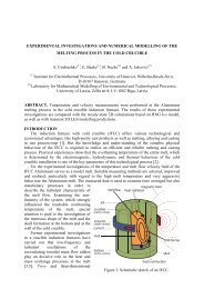
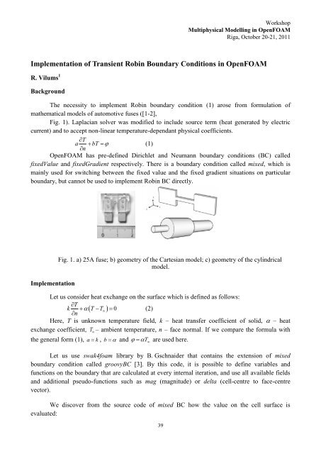
The necessity to implement Robin boundary condition (1) arose from formulation of
mathematical models of automotive fuses ([1-2],
Fig. 1). Laplacian solver was modified to include source term (heat generated by electric
current) and to accept non-linear temperature-dependant physical coefficients.
T
a
bT
(1)
n
OpenFOAM has pre-defined Dirichlet and Neumann boundary conditions (BC) called
fixedValue and fixedGradient respectively. There is a boundary condition called mixed, which is
mainly used for switching between the fixed value and the fixed gradient situations on particular
boundary, but cannot be used to implement Robin BC directly.
Implementation
Fig. 1. a) 25A fuse; b) geometry of the Cartesian model; c) geometry of the cylindrical
model.
Let us consider heat exchange on the surface which is defined as follows:
T
k T T 0
n
(2)
Here, T is unknown temperature field, k – heat transfer coefficient of solid, – heat
exchange coefficient, T
– ambient temperature, n – face normal. If we compare the formula with
the general form (1), a k, b and T are used here.
Let us use swak4foam library by B. Gschnaider that contains the extension of mixed
boundary condition called groovyBC [3]. By this code, it is possible to define variables and
functions on the boundary that are calculated at every internal iteration, and use all available fields
and additional pseudo-functions such as mag (magnitude) or delta (cell-centre to face-centre
vector).
We discover from the source code of mixed BC how the value on the cell surface is
evaluated:
39

T f valueExpr f T gradExpr ,
face
(1 )
centre
where f is fractionExpression defined by user and – distance between the cell centre and
cell face.
obtain:
If we linearise the derivative in the formula (2) by
1
T
face
and T
centre
, and isolate T
face
, we
Tface
fT
1 f T
, k
center f 1
. (3)
Comparison with the previous expression shows how to implement this BC in a code.
outerSurface
{
}
type groovyBC;
variables "k=0.2;alpha=15;Tinf=65; f=1/(1+k/(alpha*mag(delta())));";
valueExpression "Tinf";
gradientExpression "0";
fractionExpression "f";
value uniform 0;
Constants k, and T
were used here. For the transient parameters, it is recommended to
define and calculate them in a solver as fields or calculate directly in groovyBC, e.g.
“k=0.2+0.03*T+4e-5*pow(T,3)”.
Acknowledgement
This work was supported by the ESF Project No. 2009/0223/1DP/1.1.1.2.0/APIA/VIAA/008
References
Vilums, R., Buikis, A. Conservative Averaging and Finite Difference Methods for Transient Heat
Conduction in 3D Fuse. WSEAS Transactions on Heat and Mass Transfer. 3(1):111-124, 2008.
Vilums, R., Liess, H.-D., Buikis, A., Rudevics A. Cylindrical Model of Transient Heat Conduction
in Automotive Fuse Using Conservative Averaging Method. The 13 th WSEAS Int. Conf. on Applied and
Computational Mathematics, Puerto De La Cruz, Tenerife, Spain, 355-360, 2008.
Gschaider, B. Swak4Foam [Online: http:// openfoamwiki.net/index.php/Contrib/swak4Foam]
1 University of Latvia, Faculty of Physics and Mathematics, Zellu iela 8, Riga, LV-1459, Latvia
40