pdf version - Oomph-lib

Chapter 1 

Boussinesq Convection: Combining the 

Navier–Stokes and Advection–Diffusion 

equations 

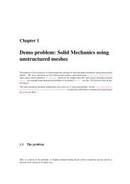
Figure 1.1: Steady Convection Rolls: contours of temperature and the vector velocity field for a twodimensional 

domain heated from below at Ra = 1800 

We study convection of an incompressible Newtonian fluid heated from below in a two-dimensional domain 

of height H: the Bénard problem. The lower wall is maintained at a temperature θ bottom and the upper 

wall is maintained at a temperature θ top , where θ bottom > θ top . The governing equations are the (2D) 

Navier–Stokes equations under the Boussinesq approximation, in which all variations in physical properties 

with temperature are neglected, apart from that of the density in the gravitational-body-force term in the 

momentum equations. This "buoyancy" term is given by 

∆ρG ∗ i , 

where ∆ρ is the variation in density and G ∗ i is the i -th component of the gravitational body force. Under 

the additional assumption that variations in temperature are small, we can use the linear relationship 

∆ρ = −αρ 0 (θ ∗ − θ 0 ), 

where α is the coefficient of thermal expansion of the fluid, θ ∗ is the (dimensional) temperature and ρ 0 is 

the density at the reference temperature θ 0 .

2 Boussinesq Convection: Combining the Navier–Stokes and Advection–Diffusion equations 

The equations governing the fluid motion are thus the Navier–Stokes equations with the inclusion of the 

additional buoyancy term. In Cartesian coordinates, we have 

( 

∂u ∗ i 

ρ 0 

∂t ∗ + u∗ j 

∂u ∗ i 

∂x ∗ j 

) 

= − ∂p∗ 

∂x ∗ i 

[ 

+ [ρ 0 − αρ 0 (θ ∗ − θ 0 )] G ∗ ∂ ∂u ∗ i 

i + µ 0 

∂x ∗ j ∂x ∗ j 

+ ∂u∗ j 

∂x ∗ i 

] 

, 

and 

∂u ∗ i 

∂x ∗ i 

Here, u ∗ i is the i -th (dimensional) velocity component and x∗ i is the position in the i-th coordinate direction; 

µ 0 is the dynamic viscosity of the fluid at the reference temperature and t ∗ is the dimensional time. 

The equation that governs the evolution of the temperature field is the advection-diffusion equation where 

the "wind" is the fluid velocity. Thus, 

= 0. 

∂θ ∗ 

∂t ∗ + ∂θ ∗ 

u∗ j 

∂x ∗ j 

( 

= κ ∂ ∂θ ∗ 

∂x ∗ j ∂x ∗ j 

) 

, 

where κ is the (constant) thermal diffusivity of the fluid. 

We choose the height of the domain, H, as the length scale and let the characteristic thermal diffusion 

speed over that length, κ/H, be the velocity scale, so that the Péclet number, P e = UH/κ = 1 . The 

fluid pressure is non-dimensionalised on the viscous scale, µ 0 κ/H 2 , and the hydrostatic pressure gradient 

is included explicitly, so that we work with the dimensionless excess pressure. The temperature is nondimensionalised 

so that it is -0.5 at the upper (cooled) wall and 0.5 at the bottom (heated) wall and the 

reference temperature is then θ 0 = (θ top + θ bottom )/2. Finally, the timescale is chosen to be the thermal 

diffusion timescale, κ/H 2 . Hence 

x ∗ i = x i H, u ∗ i = u i κ/H, p ∗ = −ρ 0 gHx 2 + µ 0κ 

H 2 p, θ∗ = θ 0 + θ(θ bottom − θ top ), t ∗ = κ H 2 t. 

The governing equations become 

( ) 

P r −1 ∂ui 

∂t + u ∂u i 

j 

∂x j 

= − ∂p 

∂x i 

− RaθG i + 

∂u i 

∂x i 

= 0, 

and 

∂θ 

∂t + u ∂θ 

j = 

∂ ( ) ∂θ 

, 

∂x j ∂x j ∂x j 

. 

∂ [ ∂ui 

+ ∂u ] 

j 

, 

∂x j ∂x j ∂x i 

The appropriate dimensionless numbers are the Prandtl number P r = ν κ 

, and the Rayleigh number, Ra = 

α(θ bottom −θ top)gH 3 

νκ 

; g is the acceleration due to gravity and ν = µ 0 /ρ 0 is the kinematic viscosity of the 

fluid. 

Generated on Mon Aug 10 11:45:56 2009 by Doxygen

3 

We consider the solution of this coupled set of equations in a two-dimensional domain 0 ≤ x 1 ≤ 3 , 

0 ≤ x 2 ≤ 1 . The boundary conditions are no-slip at the top and bottom walls 

u 1 = u 2 = 0 on x 2 = 0, 1; 

constant temperature at the top and bottom walls (heated from below) 

and symmetry boundary conditions at the sides: 

θ = 0.5 on x 2 = 0 and θ = −0.5 on x 2 = 1; 

u 1 = 0, 

∂u 2 

∂x 1 

= 0, 

and ∂θ 

∂x 1 

= 0 on x 1 = 0, 3. 

We assume that gravity acts vertically downward so that G 1 = 0 and G 2 = −1 . 

There is a trivial steady-state solution that consists of a linearly-varying temperature field balanced by a 

quadratic pressure field: 

u 1 = u 2 = 0, θ = 0.5 − x 2 , p = P 0 + 0.5 Ra x 2 (1 − x 2 ) . 

Figure 1.2: The base flow: no flow and a linear temperature distribution 

A linear stability analysis shows that this solution becomes unstable via an up-down, symmetry-breaking, 

pitchfork bifurcation at a critial Rayleigh number of Ra crit ≈ 1708 with a critical wavenumber of 

k ≈ 3.11, see for example Hydrodynamic and Hydromagnetic Stability by S. Chandrasekhar OUP (1961). 

Thus, for Ra > 1708 there are three possible steady solutions, the (unstable) trivial steady state and two 

(stable) symmetry-broken states. In principle, all three states can be computed directly by solving the 

steady equations. However, we typically find that if the steady computation is started with a zero initial 

guess for the velocity and temperature, the Newton method converges to the trivial state. In order to demonstrate 

that this state is indeed unstable we therefore apply a time-dependent, mass-conserving perturbation 

to the vertical velocity at the upper wall and time-march the system while rapidly reducing the size of the 

perturbation. The system then evolves towards the nontrivial steady state as shown in the animation 

from which the plots shown above were extracted. (In the next tutorial where we discuss 

the adaptive solution of this problem we shall demonstrate an alternative technique for 

obtaining this solutions). 

Note that by choosing our domain of a particular size and applying symmetry conditions at the sidewalls 

we are only able to realise a discrete set of wavelengths (those that exactly fit into the box). At the chosen 

Rayleigh number, 1800, only one of these modes is unstable; that of wavelength 2. 



1.1 Global parameters and functions 

The problem contains three global parameters, the Péclet number, the Prandtl number and the Rayleigh 

number which we define in a namespace, as usual. In fact, 1/P r is the natural dimensionless grouping, 

and so we use the inverse Prandtl number as our variable. 

//======start_of_namespace============================================ 

/// Namespace for the physical parameters in the problem 

//==================================================================== 

namespace Global_Physical_Variables 

{ 

/// Peclet number (identically one from our non-dimensionalisation) 

double Peclet=1.0; 

/// 1/Prandtl number 

double Inverse_Prandtl=1.0; 

/// \short Rayleigh number, set to be greater than 

/// the threshold for linear instability 

double Rayleigh = 1800.0; 

/// Gravity vector 

Vector Direction_of_gravity(2); 

} // end_of_namespace 

1.2 The driver code 

In the driver code we set the direction of gravity and construct our problem, using the new Buoyant- 

QCrouzeixRaviartElement, a multi-physics element, created by combining the QCrouzeixRaviart 

Navier-Stokes elements with the QAdvectionDiffusion elements via multiple inheritance. (Details 

of the element’s implementation are discussed in the section Creating the new BuoyantQCrouzeixRaviart- 

Element class below.) 

//=======start_of_main================================================ 

/// Driver code for 2D Boussinesq convection problem 

//==================================================================== 

int main(int argc, char **argv) 

{ 

// Set the direction of gravity 

Global_Physical_Variables::Direction_of_gravity[0] = 0.0; 

Global_Physical_Variables::Direction_of_gravity[1] = -1.0; 

//Construct our problem 

ConvectionProblem problem; 

We assign the boundary conditions at the time t = 0 and initially perform a single steady solve to obtain the 

trivial (and temporally unstable) trivial solution; see the section Comments for a more detailed discussion 

of the Problem::steady_newton_solve() function. 

// Apply the boundary condition at time zero 

problem.set_boundary_conditions(0.0); 

//Perform a single steady Newton solve 

problem.steady_newton_solve(); 

//Document the solution 

problem.doc_solution(); 


1.3 The problem class 5 

The result of this calculation is the trivial symmetric base flow. We next timestep the system using the 

(unstable) steady solution as the initial condition. As time increases, the flow evolves to one of the stable 

asymmetric solutions, as shown in the animation of the results. As usual, we only perform a 

few timesteps when the code is used as a self-test, i.e. if any command-line parameters are passed to the 

driver code. 

//Set the timestep 

double dt = 0.1; 

//Initialise the value of the timestep and set an impulsive start 

problem.assign_initial_values_impulsive(dt); 

//Set the number of timesteps to our default value 

unsigned n_steps = 200; 

//If we have a command line argument, perform fewer steps 

//(used for self-test runs) 

if(argc > 1) {n_steps = 5;} 

//Perform n_steps timesteps 

for(unsigned i=0;i


// Domain length in y-direction 

double l_y=1.0; 

// Build a standard rectangular quadmesh 

Problem::mesh_pt() = 

new RectangularQuadMesh(n_x,n_y,l_x,l_y,time_stepper_pt()); 

Next, the boundary constraints are imposed. We pin all velocities and the temperature on the top and bottom 

walls and pin only the horizontal velocity on the sidewalls. Since the domain is enclosed, the pressure is 

only determined up the an arbitrary constant. We resolve this ambiguity by pinning a single pressure value, 

using the fix_pressure(...) function. 

// Set the boundary conditions for this problem: All nodes are 

// free by default -- only need to pin the ones that have Dirichlet 

// conditions here 

//Loop over the boundaries 

unsigned num_bound = mesh_pt()->nboundary(); 

for(unsigned ibound=0;iboundnboundary_node(ibound); 

for (unsigned inod=0;inodpin(j); 

} 

} 

} 

//Pin the zero-th pressure dof in element 0 and set its value to 

//zero: 

fix_pressure(0,0,0.0); 

We complete the build of the elements by setting the pointers to the physical parameters and finally assign 

the equation numbers 

unsigned n_element = mesh_pt()->nelement(); 

for(unsigned i=0;ielement_pt(i)); 

// Set the Peclet number 

el_pt->pe_pt() = &Global_Physical_Variables::Peclet; 

// Set the Peclet number multiplied by the Strouhal number 

el_pt->pe_st_pt() =&Global_Physical_Variables::Peclet; 

// Set the Reynolds number (1/Pr in our non-dimensionalisation) 

el_pt->re_pt() = &Global_Physical_Variables::Inverse_Prandtl; 

// Set ReSt (also 1/Pr in our non-dimensionalisation) 

el_pt->re_st_pt() = &Global_Physical_Variables::Inverse_Prandtl; 


1.3 The problem class 7 

// Set the Rayleigh number 

el_pt->ra_pt() = &Global_Physical_Variables::Rayleigh; 

//Set Gravity vector 

el_pt->g_pt() = &Global_Physical_Variables::Direction_of_gravity; 

//The mesh is fixed, so we can disable ALE 

el_pt->disable_ALE(); 

// Set pointer to the continuous time 

el_pt->time_pt() = time_pt(); 

} 

// Setup equation numbering scheme 

cout


double epsilon = 0.01; 

//Read out the x position 

double x = nod_pt->x(0); 

//Set a sinusoidal perturbation in the vertical velocity 

//This perturbation is mass conserving 

double value = sin(2.0*MathematicalConstants::Pi*x/3.0)* 

epsilon*time*exp(-time); 

nod_pt->set_value(1,value); 

} 

//If we are on the bottom boundary, set the temperature 

//to 0.5 (heated) 

if(ibound==0) {nod_pt->set_value(2,0.5);} 

} 

} 

} // end_of_set_boundary_conditions 

1.3.3 The function fix_pressure(...) 

This function is a simple wrapper to the element’s fix_pressure(...) function. 

///Fix pressure in element e at pressure dof pdof and set to pvalue 

void fix_pressure(const unsigned &e, const unsigned &pdof, 

const double &pvalue) 

{ 

//Cast to specific element and fix pressure 

dynamic_cast(mesh_pt()->element_pt(e))-> 

fix_pressure(pdof,pvalue); 

} // end_of_fix_pressure 

1.3.4 The function actions_before_implicit_timestep() 

This function is used to ensure that the time-dependent boundary conditions are set to the correct value 

before solving the problem at the next time level. 

/// \short Actions before the timestep (update the the time-dependent 

/// boundary conditions) 

void actions_before_implicit_timestep() 

{ 

set_boundary_conditions(time_pt()->time()); 

} 

1.3.5 The function doc_solution(...) 

This function writes the complete velocity, pressure and temperature fields to a file in the output directory. 

//===============start_doc_solution======================================= 

/// Doc the solution 

//======================================================================== 

template 

void ConvectionProblem::doc_solution() 

{ 

//Declare an output stream and filename 

ofstream some_file; 

char filename[100]; 

// Number of plot points: npts x npts 


1.4 Creating the new BuoyantQCrouzeixRaviartElement class 9 

unsigned npts=5; 

// Output solution 

//----------------- 

sprintf(filename,"%s/soln%i.dat",Doc_info.directory().c_str(), 

Doc_info.number()); 

some_file.open(filename); 

mesh_pt()->output(some_file,npts); 

some_file.close(); 

Doc_info.number()++; 

} // end of doc 

1.4 Creating the new BuoyantQCrouzeixRaviartElement class 

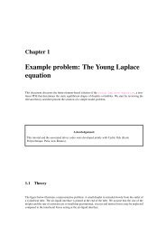
The sketch below illustrates how the new multi-physics BuoyantQCrouzeixRaviartElement is 

constructed by multiple inheritance from the two existing single-physics elements: 

Figure 1.3: Sketch illustrating the construction of the BuoyantQCrouzeixRaviartElement by multiple inheritance. 

• The nine-noded two-dimensional QCrouzeixRaviartElement is based on a nine-node quadrilateral 

geometric FiniteElement from the QElement family. All of its Nodes store two values, 

the horizontal and vertical velocity, respectively. The element also stores internal Data which represents 

the (discontinuous) pressure degrees of freedom; in the sketch this Data is represented by 

the dashed box. 

• The two-dimensional QAdvectionDiffusionElement is based on the same geometric 

FiniteElement and stores one value (the temperature, θ ) at each Node. 

Both elements are fully-functional and provide their contributions to the global system of nonlinear 

algebraic equations that is solved by Newton’s method via the two member functions fill_in_- 

contribution_to_residuals(...) and fill_in_contribution_to_jacobian(...). 



• The QAdvectionDiffusionElement’s member function fill_in_contribution_- 

to_residuals(...) computes the element’s contribution to the global residual vector for a 

given "wind". The "wind" is specified by its virtual member function get_wind_adv_diff(...) 

and in the single-physics advection diffusion problems studied so far, 

the "wind" tended to specified a priori by the user. The element’s member function fill_in_- 

contribution_to_jacobian(...) computes the elemental Jacobian matrix, i.e. the derivatives 

of the elemental residual vector with respect to its unknown nodal values (the temperatures). 

• Similarly, the QCrouzeixRaviartElement’s member function fill_in_- 

contribution_to_residuals(...) computes the element’s contribution to the global 

residual vector for a given body force. The body force is specified by its virtual member function 

get_body_force_nst(...) and in the single-physics Navier-Stokes problems 

studied so far, the body force tended to specified a priori by the user. The element’s member 

function fill_in_contribution_to_jacobian(...) computes the elemental Jacobian 

matrix, i.e. the derivatives of the elemental residual vector with respect to its unknown nodal and 

internal values (the velocities and the pressure). 

When combining the two single-physics elements to a multi-physics element, we have to take the interaction 

between the constituent equations into account: In the coupled problem the "wind" in the advectiondiffusion 

equations is given by the Navier-Stokes velocities, while the body force in the Navier-Stokes 

equations is a function of the temperature. When implementing these interactions we wish to recycle as 

much of the elements’ existing functionality as possible. This may be achieved by the following straightforward 

steps: 

1. Construct the combined multi-physics element by multiple inheritance. 

2. Overload the FiniteElement::required_nvalue(...) function to ensure that each Node 

provides a sufficient amount of storage for the (larger) number of nodal values required in the multiphysics 

problem. 

3. Overload the constituent element’s member functions that indicate which nodal value corresponds to 

which type of degree of freedom. For instance, in the single-physics advection-diffusion problem, 

the temperature is stored at the zero-th nodal value whereas in the combined multi-physics element, 

the temperature is stored as the second value, as shown in the above sketch. 

4. Provide a final overload for the element’s fill_in_contribution_to_residuals(...) and 

fill_in_contribution_to_jacobian(...) functions. The former simply concatenates the 

residual vectors computed by the constituent single-physics elements. The latter function is easiest 

to implement by finite differencing the combined element’s residual vector. [A more efficient approach 

(in terms of cpu time, not necessarily terms of development time!) is to recycle the diagonal 

blocks computed by the constituent elements’s fill_in_contribution_to_jacobian(...) 

functions and to use finite-differencing only for the off-diagonal (interaction) blocks; see the section 

Comments a more detailed discussion of this technique.] 

That’s all! Here is the implementation: 

//======================class definition============================== 

///A class that solves the Boussinesq approximation of the Navier--Stokes 

///and energy equations by coupling two pre-existing classes. 

///The QAdvectionDiffusionElement with bi-quadratic interpolation for the 

///scalar variable (temperature) and 

///QCrouzeixRaviartElement which solves the Navier--Stokes equations 

///using bi-quadratic interpolation for the velocities and a discontinuous 

///bi-linear interpolation for the pressure. Note that we are free to 

///choose the order in which we store the variables at the nodes. In this 

///case we choose to store the variables in the order fluid velocities 

///followed by temperature. We must, therefore, overload the function 


1.4 Creating the new BuoyantQCrouzeixRaviartElement class 11 

///AdvectionDiffusionEquations::u_index_adv_diff() to indicate that 

///the temperature is stored at the DIM-th position not the 0-th. We do not 

///need to overload the corresponding function in the 

///NavierStokesEquations class because the velocities are stored 

///first. 

//========================================================================= 

template 

class BuoyantQCrouzeixRaviartElement : 

public virtual QAdvectionDiffusionElement, 

public virtual QCrouzeixRaviartElement 

The class contains a single new physical parameter, the Rayleigh number, as usual referenced by a pointer 

to a double precision datum, 

/// Pointer to a private data member, the Rayleigh number 

double* Ra_pt; 

with suitable access functions. 

///Access function for the Rayleigh number (const version) 

const double &ra() const {return *Ra_pt;} 

///Access function for the pointer to the Rayleigh number 

double* &ra_pt() {return Ra_pt;} 

The constructor calls the constructors of the component classes (QCrouzeixRaviartElement and 

QAdvectionDiffusionElement) and initialises the value of the Rayleigh number to zero, via a 

static default parameter value. 

/// \short Constructor: call the underlying constructors and 

/// initialise the pointer to the Rayleigh number to point 

/// to the default value of 0.0. 

BuoyantQCrouzeixRaviartElement() : QAdvectionDiffusionElement(), 

QCrouzeixRaviartElement() 

{ 

Ra_pt = &Default_Physical_Constant_Value; 

} 

We must overload the function FiniteElement::required_nvalue() because the new element 

will store DIM+1 unknowns at each node: DIM fluid velocity components and the value of the temperature, 

as shown in the sketch above. 

///\short The required number of values stored at the nodes is the sum of the 

///required values of the two single-physics elements. Note that this step is 

///generic for any multi-physics element of this type. 

unsigned required_nvalue(const unsigned &n) const 

{return (QAdvectionDiffusionElement::required_nvalue(n) + 

QCrouzeixRaviartElement::required_nvalue(n));} 

In the standard single-physics advection-diffusion elements the temperature is the only value stored at the 

nodes and is stored as value(0). Similarly, in the single-physics Navier–Stokes elements, the fluid velocities 

are stored in the first DIM nodal values. In our new multi-physics element, we must decide where to 

store the different variables and then inform the single-physics elements of our choice. As indicated in the 

above sketch, we choose to store the temperature after the fluid velocities, so that it is value(DIM). The 

recommended mechanism for communicating the location of the variables to the single-physics elements 

is to use an index function. Hence, single-physics elements that are to be the components of multi-physics 

elements must have an index function for their variables. For instance, the function u_index_adv_- 

diff(...) is used in the AdvectionDiffusionEquations class to read out the position (index) at 

which the advected variable (the temperature) is stored. That function is now overloaded in our multiphysics 

element: 



///\short Overload the index at which the temperature 

///variable is stored. We choose to store it after the fluid velocities. 

inline unsigned u_index_adv_diff() const {return DIM;} 

We need not overload the index function for the fluid velocities because they remain stored in the first DIM 

positions at the node. 

The coupling between the two sets of single-physics equations is achieved by overloading the two functions 

get_wind_adv_diff(), used in the advection-diffusion equations and get_body_force_nst(), 

used in the Navier–Stokes equations 

/// \short Overload the wind function in the advection-diffusion equations. 

/// This provides the coupling from the Navier--Stokes equations to the 

/// advection-diffusion equations because the wind is the fluid velocity. 

void get_wind_adv_diff(const unsigned& ipt, 

const Vector &s, const Vector& x, 

Vector& wind) const 

{ 

//The wind function is simply the velocity at the points 

this->interpolated_u_nst(s,wind); 

} 

/// \short Overload the body force in the Navier-Stokes equations 

/// This provides the coupling from the advection-diffusion equations 

/// to the Navier--Stokes equations, the body force is the 

/// temperature multiplied by the Rayleigh number acting in the 

/// direction opposite to gravity. 

void get_body_force_nst(const double& time, const unsigned& ipt, 

const Vector &s, const Vector &x, 

Vector &result) 

{ 

//Get the temperature 

const double interpolated_t = this->interpolated_u_adv_diff(s); 

// Get vector that indicates the direction of gravity from 

// the Navier-Stokes equations 

Vector gravity(NavierStokesEquations::g()); 

// Temperature-dependent body force: 

for (unsigned i=0;i

1.5 Comments and Exercises 13 

the FiniteElement base class: 

///\short Compute the element’s residual vector and the Jacobian matrix. 

/// Jacobian is computed by finite-differencing. 

void fill_in_contribution_to_jacobian(Vector &residuals, 

DenseMatrix &jacobian) 

{ 

// This function computes the Jacobian by finite-differencing 

FiniteElement::fill_in_contribution_to_jacobian(residuals,jacobian); 

} 

Finally, we overload the output function to print the fluid velocities, the fluid pressure and the temperature. 

// Start of output function 

void output(ostream &outfile, const unsigned &nplot) 

{ 

//vector of local coordinates 

Vector s(DIM); 

// Tecplot header info 

outfile tecplot_zone_string(nplot); 

// Loop over plot points 

unsigned num_plot_points=this->nplot_points(nplot); 

for (unsigned iplot=0;iplotget_s_plot(iplot,nplot,s); 

// Output the position of the plot point 

for(unsigned i=0;i


all unknown Data values will have been assigned their correct values so that the solution of 

the problem may be plotted by calls to the elements’ output functions. We tended to use this 

function to solve steady problems. 

– Given the solution at time t = t orig , the unsteady Newton solver Problem::unsteady_- 

newton_solve(dt,...) increments time by dt, shifts the "history" values and then 

computes the solution at the advanced time, t = t orig + dt. On return from this function, 

all unknown Data values (and the corresponding "history" values) will have been assigned 

their correct values so that the solution at time t = t orig + dt may be plotted by calls to the 

elements’ output functions. We tended to use this function for unsteady problems. 

Inspection of the Problem::unsteady_newton_solve(...) function shows that this function 

is, in fact, a wrapper around Problem::newton_solve(), and that the latter function solves 

the discretised equations including any terms that arise from an implicit time-discretisation. The 

only purpose of the wrapper function is to shift the history values before taking the next timestep. 

This raises the question how to compute steady solutions (i.e. solutions obtained by setting the 

time-derivatives in the governing equation to zero) of a Problem that was discretised in a form 

that allows for timestepping, as in the problem studied here. This is the role of the function 

Problem::steady_newton_solve(): The function performs the following steps: 

1. Disable all TimeSteppers in the Problem by calling their TimeStepper::make_- 

steady() member function. 

2. Call the Problem::newton_solve() function to compute the solution of the discretised 

problem with all time-derivatives set to zero. 

3. Re-activate all TimeSteppers (unless they were already in "steady" mode when the function 

was called). 

4. Call the function Problem::assign_initial_values_impulsive() to ensure that 

the "history" values used by the (now re-activated) TimeSteppers are consistent with an 

impulsive start from the steady solution just computed. 

On return from this function, all unknown Data values (and the corresponding "history" values) will 

have been assigned their correct values so that the solution just computed is a steady solution to the 

full unsteady equations. 

• Optimising the implementation of multi-physics interactions: 

The combined multi-physics element discussed above was implemented with just a few straightforward 

lines of code. The ease of implementation comes at a price, however, and more efficient 

implementations (in terms of CPU time) are possible: 

1. Using finite-differencing only for the off-diagonal terms in the Jacobian matrix: 

While the use of finite-differencing in the setup of the Jacobian matrix is convenient, it does 

not exploit the fact that the constituent single-physics elements already provide analytical 

(and hence cheaper-to-compute) expressions for the two diagonal blocks in the coupled Jacobian 

matrix (i.e. the derivatives of the fluid residuals with respect to the fluid variables, 

and the derivatives of the advection diffusion residuals with respect to the temperature degrees 

of freedom). It is possible to recycle these entries and to use finite-differencing only 

to compute the off-diagonal interaction blocks (i.e. the derivatives of the Navier-Stokes 

residuals with respect to the temperature degrees of freedom, and the derivatives of the 

advection-diffusion residuals with respect to the velocities). In fact, the source code for the 

BuoyantQCrouzeixRaviartElement includes such an implementation. The full finitedifference-based 

computation discussed above is used if the code is compiled with the compiler 

flag USE_FD_JACOBIAN_FOR_BUOYANT_Q_ELEMENT. Finite-differences are used for the 

off-diagonal blocks only when the compiler flag USE_OFF_DIAGONAL_FD_JACOBIAN_- 

FOR_BUOYANT_Q_ELEMENT is passed. When comparing the two versions of the code, we 


1.6 Source files for this tutorial 15 

found the run times for the full finite-difference-based version to be approximately 3-7% higher, 

depending on the spatial resolution used. The implementation of the more efficient version is 

still straightforward and can be found in the source code boussinesq_convection.cc. 

2. Using an analytic Jacobian matrix: 

As discussed above, the re-use of the analytic expressions for the diagonal blocks of the coupled 

Jacobian matrix is straightforward. For a yet more efficient computation we can assemble 

analytic expressions for the off-diagonal interaction blocks; although this does require knowledge 

of precisely how the governing equations were implemeted in the single-physics elements. 

Once again, the source code for the BuoyantQCrouzeixRaviartElement includes such 

an implementation and, moreover, it is the default behaviour. We found the assembly time 

for the analytic coupled Jacobian to be approximately 15% of the finite-difference based versions. 

The implementation is reasonably straightforward and can be found in the source code 

boussinesq_convection.cc. 

3. Complete re-implementation of the coupled element: 

Although recycling the analytically computed diagonal blocks in the Jacobian matrix leads 

to a modest speedup, and the use of analytic off-diagonal blocks to a further speedup, the 

computation of the coupled residual vector and Jacobian matrix are still somewhat inefficient. 

This is because the contributions from the Navier-Stokes and advection-diffusion equations are 

computed in two separate integration loops; and, if computed, the assembly of the analytic 

off-diagonal terms requires a third integration loop. The only solution to this problem would 

be to fully merge the source codes for two elements to create a customised element. In the 

present problem this would not be too difficult, particularly since the derivatives of the Navier- 

Stokes residuals with respect to the temperature, and the derivatives of the advection-diffusion 

residuals with respect to the velocities are easy to calculate. However, a reimplementation in 

this form would break the modularity of the library as any subsequent changes/improvements 

to the Navier-Stokes elements, say, would have to be added manually to the coupled element. 

If maximum speed is absolutely essential in your application, you may still wish to choose 

this option. The existing Navier-Stokes and advection diffusion elements provide the required 

building blocks for your custom-written coupled element. 

1.5.2 Exercises 

1. Confirm that the system is stable, i.e. returns to the trivial state, when Ra = 1700 . 

2. How does the time-evolution of the system change when no-slip boundary conditions for the fluid 

velocity are applied on the side boundaries (a rigid box model)? 

3. Re-write the multi-physics elements so that the temperature is stored before the fluid velocities. 

Confirm that the solution is unchanged in this case. 

4. Assess the computational cost of the finite-difference based setup of the elements’ Jacobian matrices 

by comparing the run times of the two versions of the code. 

5. Try using QTaylorHoodElements as the "fluid" element part of the multi-physics elements. 

N.B. in this case, the temperature must be stored as the first variable at the nodes because we assume 

that it is always stored at the same location in every node. 

1.6 Source files for this tutorial 

• The source files for this tutorial are located in the directory: 



• The driver code is: 

demo_drivers/multi_phsyics/boussinesq_convection/ 

demo_drivers/multi_physics/boussinesq_convection/boussinesq_- 

convection.cc 

1.7 PDF file 

A pdf version of this document is available.

pdf version - Oomph-lib

You also want an ePaper? Increase the reach of your titles

Delete template?

Save as template?