Diffusion Manual Outline
Diffusion Manual Outline
Diffusion Manual Outline

Create successful ePaper yourself
Turn your PDF publications into a flip-book with our unique Google optimized e-Paper software.
1<br />
MEASURING DIFFUSION BY NMR<br />
Bruker Instruments Inc.<br />
Sophie Kazanis<br />
Application Scientist<br />
August 2000
2<br />
Table of Contents<br />
Chapter 1<br />
Section 1.1<br />
Section 1.2<br />
Section 1.3<br />
Chapter 2<br />
Chapter 3<br />
Section 3.1<br />
Section 3.2<br />
Section 3.3<br />
Section 3.4<br />
Introduction to <strong>Diffusion</strong><br />
Introduction<br />
Some Theory<br />
Measuring <strong>Diffusion</strong><br />
Hardware and Probe Configuration<br />
Measuring <strong>Diffusion</strong><br />
Preparation<br />
Acquisition<br />
DOSY Data Analysis using ILT<br />
DOSY Data Analysis using XWINNMR:<br />
Fitting <strong>Diffusion</strong> Coefficients<br />
Appendix
3<br />
Chapter 1<br />
Section 1.1<br />
Introduction to <strong>Diffusion</strong><br />
Introduction<br />
Self-diffusion is a measure of the translational motion of a molecule. <strong>Diffusion</strong> is<br />
closely related to molecular size as illustrated by the Stokes-Einstein equation seen<br />
below:<br />
D = k T<br />
f<br />
where k is the Boltzman constant, T is the temperature and f is the friction coefficient.<br />
For the simple case of a spherical particle of a hydrodynamic radius r s in a solvent of<br />
viscosity η, the friction factor is given by f = 6 π η r s<br />
Translational diffusion can be used to determine the size and shape of individual<br />
molecules as well as molecular aggregates. This provides an excellent way of analyzing<br />
complex mixtures without having to physically separate out each individual component.<br />
Pulsed-field gradient (PFG) NMR can be used to measure translational diffusion<br />
by applying externally controlled magnetic field gradients. These gradients spatially<br />
encode the position of each nuclear spin. This spatial distribution can be decoded after<br />
waiting a short time by applying a second gradient. If the waiting time is very short<br />
between the encoding and decoding gradients the spins will not have had a chance to<br />
change position and in turn the magnetization will refocus without a net phase change.<br />
However the spins that have moved during the waiting time between the encoding and<br />
decoding steps will acquire a net phase change. The summation of the accumulated<br />
phases over the entire sample will lead to partial cancellation of the observable<br />
magnetization and hence an attenuation of the NMR signal. This signal attenuation is<br />
dependent on the strength of the applied gradients, the time between the gradients<br />
(diffusion time) and the diffusion coefficient of the molecules under study.<br />
Section 1.2<br />
Some Theory<br />
Nuclear spins within a homogeneous magnetic field precess at the Larmor<br />
frequency according to the equation<br />
ω o = γB o<br />
where ω o is the Larmor frequency<br />
γ is the gyromagnetic ratio and<br />
B o is the strength of the magnetic field
4<br />
An external field gradient, g, can be described by the equation<br />
g = ∂ B z i + ∂ B z j + ∂ B z k<br />
∂x ∂y ∂z<br />
where i, j and k are unit vectors in the x, y and z direction.<br />
When an external gradient is applied the magnetic field at a specific set of coordinate can<br />
be described as the sum of the main field and the field due to the applied gradient:<br />
B = B o + g . r<br />
where r describes the position of a specific nuclear spin<br />
The direction of the magnetic field is usually defined as the z-direction. Here we will<br />
limit our discussion to the case of a gradient applied in the z-direction. The description<br />
of the external gradient can be simplified to be<br />
g z = g . k<br />
Applying a gradient along the z direction induces change in the phase angle for each spin<br />
at a specific z coordinate. This change in phase can be described as follows:<br />
φ (z) = γ g z z t<br />
where γ is the gyromagnetic ratio, g z is the gradient strength at position z, z indicates the<br />
position of the spin at time t.<br />
The total change in phase angle of a particular spin at time, t, after a gradient has been<br />
applied is a combination of the phase change induced by the static field as well as the<br />
contribution from the applied gradient.<br />
φ (z) = γ B o t + γ g z z t<br />
Now if you apply two gradients of equal and opposite strength and duration successively<br />
after an initial 90 degree pulse, the first gradient will dephase the magnetization and the<br />
second gradient will refocus the magnetization.<br />
90º<br />
¾!UVVM<br />
ÅV²³
5<br />
Figure 1.1 Simple gradient echo experiment<br />
φ 1(z) is the phase changed by the first gradient and φ 2(z) is the phase change induced by<br />
the second gradient. The total phase accumulation is the sum of φ 1(z) and φ 2(z) .<br />
φ 1 (z) + φ 2 (z) = φ Tot(z)<br />
If the spins have not changed position during the dephasing and rephasing gradients the<br />
net total phase change will be zero and full signal should be observed.<br />
φ Tot(z) = 0<br />
In order to refocus the chemical shift evolution that occurs while the magnetization is on<br />
the transverse plane we can place a 180 degree pulse between the two gradients. Here<br />
again if the spins have not changed position during the encoding and decoding steps the<br />
net total phase change will be zero, φ Tot(z) = 0 (Note that since the 180 degree pulse<br />
inverts the magnetization, the second gradient now has to be equal in amplitude, duration<br />
and sign as the first gradient).<br />
90º 180º<br />
¾!$VVM<br />
ÅV²²<br />
Figure 1.2 Simple gradient spin echo experiment
6<br />
Section 1.3<br />
Measuring <strong>Diffusion</strong><br />
The simplest experiment that can be used to measure diffusion is the Stejskal and Tanner<br />
pulsed field gradient spin echo pulse sequence shown below.<br />
90ºx 180ºy<br />
¾!VVV$VUVWO<br />
<br />
= <br />
ÅV²VUV²UUV<br />
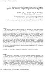
Figure 1.3 The Stejskal and Tanner PFG spin echo pulse sequence. On 1 H the thin<br />
black solid line denotes a 90º pulse and the thick solid black line denotes a 180º . G z<br />
gradients for coding and decoding are denoted by a sine bell.<br />
In this experiment a gradient is applied right after the first 90 degree pulse has been<br />
executed. The spins experience a change in the phase angle proportionate to the<br />
amplitude of the applied gradient. After a time ∆/2 a 180 degree pulse is applied which<br />
refocuses chemical shifts. The molecules are allowed to diffuse for a period of ∆. The<br />
second gradient then allows the magnetization to be refocused and the FID is<br />
subsequently recorded. Since the spins are allowed to move during the diffusion time, ∆,<br />
the net total phase change after the second gradient summed over the entire sample will<br />
not be zero. This leads to an attenuation in the observed signal.<br />
In order to measure the diffusion coefficients a series of experiments with varying echo<br />
time, ∆,=are recorded. The intensity of the signals should decrease with increasing echo<br />
time. There are two disadvantages with this method. First, the overall length of each<br />
experiment is different. Your are also usually limited with the range of echo times that<br />
can be used to obtain significant signal intensity. Secondly, the contribution of T 2<br />
relaxation during the echo time while the magnetization is on the transverse plane varies<br />
from experiment to experiment.<br />
The same effect can be obtained and the disadvantages avoided by varying the gradient<br />
amplitude while keeping the duration of the gradient constant. The overall length of each<br />
experiment will remain constant. The signal intensity will decrease with increasing<br />
gradient strength. Since the echo time for a series of experiments is the same the affects<br />
of T 2 relaxation should remain constant within a given series of experiments.
7<br />
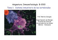
Figure 1.4 Shows the attenuation of signal with increasing gradient strength<br />
The decrease in signal intensity as a function of gradient strength can be described by the<br />
general equation<br />
I (q) = I o e-Dq2∆’<br />
where D is the diffusion coefficient<br />
∆’ = ∆ – δ/3 where<br />
∆ is the diffusion time and δ is a correction factor for finite gradients<br />
q = γgδ<br />
γ is the gyromagnetic ratio<br />
g is the amplitude of the applied gradient<br />
δ is the duration of the applied gradient<br />
A plot of I (q) versus q2 ∆’ yields an exponential decay curve which is fitted to obtain the<br />
diffusion coefficient.
8<br />
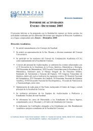
Figure 1.5 A plot of the change of signal intensity with increasing gradient strength<br />
<strong>Diffusion</strong> experiments are conveniently performed in a two dimensional fashion. A<br />
pseudo two dimensional experiment is constructed with chemical shift on the horizontal<br />
axis and (distribution of ) diffusion coefficients on the vertical axis. This is known as<br />
diffusion ordered NMR spectroscopy or DOSY.<br />
The DOSY experiment analyzes and concisely displays the data that is acquired with a<br />
series of PFG NMR experiments outlined above. The signal attenuation at each chemical<br />
shift is inverted by approximate inverse Laplace transforms (ILT) to generate a<br />
distribution of diffusion coefficients at a particular chemical shift.<br />
Figure 1.6 An example of a DOSY experiment with diffusion coefficients on the on the<br />
vertical axis and chemical shifts on the horizontal axis.
10<br />
Chapter 2<br />
Hardware and Probe Configuration<br />
To execute PFG NMR experiments your console must be equipped with a gradient<br />
control unit, GCU, and a gradient amplifier. The GREAT 1/10, GAB and single axis<br />
ACCUSTAR (10 A) amplifiers can only generate z gradients where as the ACCUSTAR<br />
and GREAT 3/10 (10 A) amplifiers can generate x, y and z gradients.<br />
All DOSY experiments can be performed with z axis gradients.<br />
The high resolution NMR probe must have a gradient coil which is actively shielded to<br />
minimize eddy currents. The gradient coil must be able to provide a constant gradient<br />
over the entire length of the active sample volume. Standard high resolution probes can<br />
generate up to 65 G/cm with a 10 A amplifier along the z axis and up to 50 G/cm along<br />
the x and y axis.<br />
Higher powered (40 A) amplifiers are available but are not recommended for standard<br />
high resolution applications.<br />
For very demanding diffusion applications special diffusion probes are available. These<br />
probes can produce up to 30 G/ cm /A or up to 1.2 kG with a 40 A amplifier. These<br />
probes have reduced high resolution performance specifications.
11<br />
Chapter 3:<br />
Section 3.1:<br />
Measuring <strong>Diffusion</strong><br />
Preparation<br />
1. You must use a 1D sequence to optimize the DOSY acquisition parameters. It is<br />
recommended that you begin with the ledbp2s1d sequence. This sequence uses<br />
bipolar gradients which help eliminate any background gradients that would lead<br />
to additional unwanted echoes. Make sure that minimum number of scans which<br />
fulfill the phase cycle are used. The initial range of diffusion time, d20, should be<br />
in the range of 50-100ms. Begin with a 1ms gradient pulse, p16, and with a<br />
gradient strength of 2%. This 1d spectrum is used as a reference.<br />
2. Increase the gradient strength to 95% and monitor the attenuation of the NMR<br />
signal. The remaining signal intensity should be approximately 2-5% of the<br />
original (reference) signal intensity. If this is not the case adjust the acquisition<br />
parameters accordingly until the above criteria are observed.<br />
3. The first variable to try adjusting is p16. For bipolar gradients p16 can be <<br />
2.5ms and for monopolar gradients p16 < 5ms. The second variable that can be<br />
modified is d20, the diffusion time.<br />
4. Once the parameters have been adjusted accordingly, you may proceed with the<br />
2D DOSY acquisition.<br />
5. If ILT will be used for the data analysis then the maximum gradient strength for<br />
the particular probe must be calibrated (see Avance GRASP users manual) and<br />
put into the file “XWINNMRHOME/conf/instr/gradient_calib”. You can do this<br />
manually from a unix shell (Notepad file Windows NT) or you can use<br />
XWINNMR by going into setpre and editing the Grad.calib.const value. The<br />
maximum gradient strength is about 60 G/cm for probes with only z-axis<br />
gradients. Probes with x,y,z-axis gradients the have maximum z-gradients of<br />
about 65 G/cm and x,y-gradients of 50 G/cm.<br />
Section 3.2:<br />
Acquisition<br />
1. Create a new dataset (edc). In the acquisition window (eda) change the PARMOD to<br />
2D.<br />
2. In the ased submenu edit the appropriate values for the pulse widths, delays,<br />
constants and sweep width.<br />
3. Execute the au program dosy by typing xau dosy. You will be asked the following<br />
questions:
12<br />
Enter the first gradient amplitude: 5<br />
Enter the final gradient amplitude: 90<br />
Enter the number of points: 16<br />
Do you want to begin the acquisition:<br />
y<br />
Typing xau dosy 5 90 16 y in the command line will have the same effect as answering<br />
the questions above.<br />
The dosy au program creates a binary linear gradient ramp file which is stored in the<br />
“~/exp/stan/nmr/lists/gp” directory and is called dramp. For this particular example the<br />
file dramp will contain a 16 step ramp starting from 5% gradient amplitude and ending<br />
with 95% and it will also automatically begin the acquisition.<br />
Dosy also creates a “vdlist” which is stored with the experiment data. This vdlist<br />
contains the gradient amplitudes in G/cm for each step of the gradient ramp. The entries<br />
in the vdlist are adjusted for the amplitude of the gradients at each step and they are also<br />
scaled to account for the fact that sine shaped gradients are used instead of rectangular<br />
gradients for the acquisition of the experiment.<br />
Other AU Programs: dosyq and dosylist<br />
The au program dosyq is similar to the au program dosy except that it creates a binary<br />
“squared” ramp file called dramp. In this case the gradient amplitudes follow a square<br />
root function. This way you would observe a linear response of signal amplitude as a<br />
function of gradient amplitude.<br />
The au program dosylist recalculates the ramp file but only stores the “vdlist” where the<br />
gradient amplitudes in G/cm units are stored. It uses the status parameters found in the<br />
experiment. You should use this au program if you did not use dosy or dosyq to start<br />
your experiment and you wish to the use ILT to process the data.
13<br />
Section 3.3:<br />
DOSY Data Analysis using ILT<br />
Figure 3.1 A comparison of the Fourier transform where the FID in the time domain is converted to an<br />
NMR experiment in the frequency domain versus the inverse Laplace transform which converts the<br />
attenuation of signal at a specific chemical shift to a distribution of diffusion coefficients.<br />
After the DOSY data has been acquired you must process it by typing xf2 on the<br />
command line. It might be necessary to apply a phase correction to the data. You should<br />
observe that the intensity of the signal amplitude decreases with increasing gradient<br />
strength.<br />
You can obtain the inverse Laplace transform (ILT) of the attenuation in signal intensity<br />
by using the Bruker ILT program.<br />
1. Type ilt on the command line. The following screen will appear.
14<br />
2. Fill out the table accordingly.<br />
First you must choose the type of pulse sequence that was used.<br />
STE is the stimulated echo pulse program (stegs1s, ledgs2s)<br />
STEbp is a stimulated echo with bipolar gradients (ledbpgs2s)<br />
DSTE is the double stimulated echo (dstegs3s)<br />
DSTEbp is a double stimulated echo with bipolar gradients<br />
Enter the new process number (procno) where the DOSY analysis will be stored. Make<br />
sure you do not overwrite the raw data.<br />
The Row start to end should indicate how many steps were in the gradient ramp file.<br />
The Col start to end should indicate the number of points representing each spectrum<br />
that will undergo the inverse Laplace transform.<br />
The threshold value indicates the lower intensity limit at a particular chemical shift for<br />
which the transformation will occur.<br />
There are three different modes offered for data analysis. The option monoexp will fit<br />
the decay of intensity at each chemical shift with single exponential decay curve and<br />
yield a single diffusion coefficient per chemical shift. This option should be used if it is<br />
known that the components within a mixture are monodisperse and a single diffusion<br />
coefficient exists. The option biexp will fit the decay of intensities with biexponential<br />
decay curve and yield a possible two diffusion coefficients per chemical shift. This<br />
option should be used if it is thought that the diffusion at each chemical shift cannot be<br />
adequately represented by a single diffusion coefficient. This would be the case if it is<br />
known that there is chemical shift overlap with various components within a mixture.<br />
The option CONTIN is used when the components within a mixture are known to be<br />
polydisperse and are known to diffuse with a distribution of coefficients. Examples of<br />
polydisperse species include polymers, micelles and droplets. So within a DOSY<br />
spectrum such species will yield Gaussian distribution of diffusion coefficients with<br />
increased width.<br />
Fit offset should be set to yes if signal intensity has not decayed to 2-5% of the original<br />
signal intensity.<br />
SI (F1) indicates how much zero filling takes place in the diffusion dimension of the<br />
pseudo 2D DOSY experiment.<br />
The value in Sdev indicates a factor by which the standard deviation is multiplied. If the<br />
experimental data has a relatively high signal to noise ratio the Sdev value can be reduced<br />
(0.01) to obtain sharper Gaussian distributions of diffusion coefficients
15<br />
Solutions bounds indicates the range of fitting parameters which are proportional to the<br />
diffusion constants. It is recommended to use the ranges 1 to 1000 or 0.1 to 100.<br />
Solution grid selects the scale in the indirect (2 nd ) (F1) dimension.<br />
3. Once the table has been filled out click on OK and read the appropriate process<br />
number.<br />
Note: Inverse Laplace transforms are very time consuming. In particular the CONTIN<br />
calculation can take several minutes to complete. If the dataset is displayed before the<br />
end of the calculation then partially transformed data will be displayed.
16<br />
Section 3.4:<br />
DOSY Data Analysis Using XWINNMR:<br />
Fitting <strong>Diffusion</strong> Coefficients<br />
1. After you have processed (xf2) and phase corrected the data you will observe a<br />
DOSY spectrum similar to the one shown below.<br />
2. Under the submenu Analysis choose Relaxation [ T1/T2 ].<br />
3. Type rspc in the command line or under Process choose Read SMX slice for<br />
peak selection. You will now observe the first 1D spectrum from the 2D dataset.<br />
4. In the utilities submenu define the peaks for which you wish to fit a diffusion<br />
curve. Select defpoints and using the middle mouse button define the peaks. Save the<br />
peak file and return to the Relaxation [ T1/T2 ] menu from the Analysis submenu.
17<br />
5. Set up the parameters for the fitting. Under the Process menu choose Setup T1<br />
parameters or type edt1 on the command line. The following screen will appear.<br />
6. Set “FITTYPE” to intensity if you only wish to use the attenuation in signal<br />
intensity for the fitting .<br />
Set “FCTYPE” to vargrad. This indicates that the diffusion experiment was<br />
acquired using variable gradients but constant time deltas.<br />
Most of the other parameters should be fine. Make sure that<br />
GAMMA (4.258 e+03 Hz/G for proton), LITDEL (p16 gradient duration) and<br />
BIGDEL (d20 diffusion time) are set correctly for that particular experiment.<br />
7. Edit the “EDGUESS”. The following screen will appear.<br />
The very top line of this menu shows the formula that is used for the fitting routine.
18<br />
The equation is in the form<br />
I (q) = I o e-Dq2∆’<br />
The fitting routine will therefore fit a single exponential decay. The fit should be quite<br />
accurate if there is a single species is represented for a particular peak at a specific<br />
chemical shift.<br />
The values GC1IO and GC1D represent the estimates for the amplitudes and the<br />
diffusion coefficients. Since the amplitudes are normalized to one GC1IO is set to 1.<br />
The estimate for the diffusion coefficient should be set to the correct order of magnitude<br />
in units m2/s. GC1D is set to 1e-09 m2/s. The values SC1IO and SC1D represent the<br />
initial steps for the fitting routing and they are usually set to on tenth of the corresponding<br />
values in the left column. SC1IO = 0.1 and SC1D = 1e-10 m2/s. Save the guesses and<br />
return to the edt1 menu. Now save the edt1 menu.<br />
8. Under the Process menu you can now Pick intensities exactly at point or you<br />
can type pdo on the command line. A graph of your data points as a function of variable<br />
gradient strength will be displayed.<br />
9. To fit the data, choose Multi-component fit from the Process menu or type<br />
simfit on the command line.
19<br />
10. To view the results on the screen the “CURPRINT” in the edo menu must be set<br />
to “$screen”. If “CURPRINT” is set to a specific printer you will get a printout of the<br />
results. The results are also stored in the processed data directory in a file called<br />
simfit.out.<br />
11. To eliminate a corrupted data point you put the cursor into the graphical window.<br />
Move the cursor to the point which you wish to remove and press the middle mouse<br />
button. Double click on the left button to exit the elimination function. Now you can fit<br />
the data again by typing simfit at the command line.
20<br />
Appendix<br />
Pulse Sequences and Corresponding Gradient Programs<br />
stegs1s<br />
The pulsed field gradient stimulated echo (PFG-STE) diffusion pulse sequence is most<br />
commonly used to measure diffusion and it is shown below. The advantage of this<br />
sequence over the classic PFG spin echo sequence is that the second 90º pulse stores the<br />
magnetization in the z direction. Now the major relaxation mechanism during the<br />
relatively long diffusion time is T 1 instead of T 2 as in the case of spin echo sequence.<br />
This is advantageous since T 1 is usually greater than T 2 for most molecules. This<br />
minimizes transverse relaxation and J-modulation affects. The subsequent 90º pulse<br />
brings the magnetization back into the xy plane for observation.<br />
90ºx 90º-x 90ºx<br />
¾!V!Vl!WUN<br />
ÅV²V)UV²UUV<br />
Figure 4.1.1 The PFG-STE pulse sequence. On 1 H the black solid lines denote 90º<br />
pulses. On Gz sine shaped gradients for coding and decoding are unfilled and spoil<br />
gradients for artifact suppression are filled with diagonal lines.<br />
The Bruker pulse program for this experiment is shown below.<br />
;stegs1s<br />
;avance-version<br />
;2D sequence for diffusion measurement using stimulated echo<br />
;using 1 spoil gradient<br />
#include <br />
#include <br />
"d31=d20-p1*2-p16-d16-p19-d16"<br />
"ds=l20"<br />
1 ze<br />
2 d1 BLKGRAD<br />
3 50u UNBLKGRAD<br />
p1 ph1<br />
GRADIENT(cnst21)<br />
d16<br />
p1 ph2<br />
GRADIENT2(cnst22)<br />
d16<br />
d31<br />
p1 ph3<br />
GRADIENT(cnst21)<br />
d16
21<br />
4u BLKGRAD<br />
go=2 ph31<br />
d1 wr #0 if #0 zd<br />
lo to 3 times td1<br />
exit<br />
ph1= 0 0 0 0 2 2 2 2 1 1 1 1 3 3 3 3<br />
ph2= 1 3 0 2<br />
ph3= 1 3 0 2<br />
ph31=0 0 2 2 2 2 0 0 3 3 1 1 1 1 3 3<br />
;pl1 : f1 channel - power level for pulse (default)<br />
;p1 : f1 channel - high power pulse<br />
;p16: gradient pulse (little DELTA)<br />
;p19: gradient pulse 2 (spoil gradient)<br />
;d1 : relaxation delay; 1-5 * T1<br />
;d16: delay for gradient recovery<br />
;d20: diffusion time (big DELTA)<br />
;d31: d20 - p1*2 - p16 - d16 - p19 - d16<br />
;l20: dummy scans (ds)<br />
;NS: 8 * n<br />
;DS: l20<br />
;td1: number of experiments<br />
;MC2: use xf2 and ilt for processing<br />
;use gradient program (GRDPROG) : Ste1s<br />
;use gradient ratio: cnst22<br />
; -13.17<br />
;use AU-program dosy or dosyq to calculate gradient-file dramp<br />
The acquisition parameters are described at the end of the pulse sequence.<br />
P1 and pl1 are the 1 H 90º pulse width and power level<br />
P16 is the duration of the encoding/decoding gradient<br />
P19 is the duration of the spoiler gradient (1-3ms)<br />
D16 is the gradient recovery time (500us)<br />
D20 is the length of the diffusion time<br />
Cnst21 represents the gradient strength of the encoding/decoding gradient. The value of<br />
cnst21 varies according to the starting and ending strength and the number of<br />
experiments indicated in the dosy au program that helps you to set up the experiment.<br />
Cnst22 is the gradient strength of the spoiler gradient and is usually set to an odd number<br />
to diminish the chances of refocusing unwanted magnetization.<br />
The gradient program that is associated with this experiment, Ste1s, is shown below:<br />
Ste1s<br />
loop l20<br />
{<br />
p16 { (0) | (0) | (0),sin(2,100) }<br />
{ (0) | (0) | (0) }<br />
p19 { (0) | (0) | (0),sin(cnst22,100) }<br />
{ (0) | (0) | (0) }<br />
p16 { (0) | (0) | (0),sin(2,100) }<br />
{ (0) | (0) | (0) }<br />
}<br />
loop td1 <br />
{<br />
loop ns<br />
{<br />
p16 { (0) | (0) | (0),sin(100,100)*dramp(100) }
22<br />
}<br />
}<br />
{ (0) | (0) | (0) }<br />
p19 { (0) | (0) | (0),sin(cnst22,100) }<br />
{ (0) | (0) | (0) }<br />
p16 { (0) | (0) | (0),sin(100,100)*dramp(100) }<br />
{ (0) | (0) | (0) }<br />
The first part of this gradient program is used during the acquisition of the dummy scans.<br />
The number of dummy scans is indicated by the variable L20.<br />
p16 { (0) | (0) | (0),sin(2,100) }<br />
indicates a sine shaped gradient pulse of 2% strength made up of 100 points.<br />
During the course of the experiment the gradient strength is varied by the value of the<br />
dramp. Dramp is set when you execute the au program ‘dosy’ and specify the starting<br />
and ending gradient strength along with the number of experiments.<br />
p16 { (0) | (0) | (0),sin(100,100)*dramp(100) }
23<br />
ledgs2s<br />
Eddy currents can effect the stimulated echo diffusion experiment. Eddy current effects<br />
occur more readily at higher gradient strengths. Using shaped gradient pulses can reduce<br />
the effects of eddy currents by decreasing the rate of change of the magnetic field when a<br />
gradient pulse is switched on or off. But using shaped gradients does not always<br />
completely alleviate the problem. The stimulated echo experiment is most affected by<br />
the eddy currents produced by the final gradient pulse. The LED, longitudinal eddy<br />
current delay sequence was developed to help minimize these affects. The fourth 90º<br />
pulse stores magnetization in the longitudinal direction, thus allowing the eddy currents<br />
to decay during the period Te (T). The fifth 90º pulse brings the magnetization back in to<br />
the transverse plane so that the FID can be acquired. The PFG-LED pulse sequence is<br />
shown below:<br />
90ºx 90º-x 90ºx 90º-x 90ºx<br />
¾!!Vl!!z!M<br />
ÅV²)UV²)UUUV<br />
Figure 4.1.2 The PFG-LED pulse sequence. On 1 H the black solid lines denote 90º pulses. On Gz sine<br />
shaped gradients for coding and decoding are unfilled and spoil gradients for artifact suppression are filled<br />
with diagonal lines.<br />
The Bruker pulse program for this experiment is shown below.<br />
;ledgs2s<br />
;avance-version<br />
;2D sequence for diffusion measurement using stimulated<br />
; echo and LED<br />
;using 2 spoil gradients<br />
;A.S. Altieri, D.P. Hinton & R.A. Byrd,<br />
; J. Am. Chem Soc. 117, 7566-7567 (1995)<br />
#include <br />
#include <br />
"d30=d21-p19-d16-4u"<br />
"d31=d20-2*p1-p16-d16-p19-d16"<br />
"ds=l20"<br />
1 ze<br />
2 d1 BLKGRAD<br />
3 50u UNBLKGRAD<br />
p1 ph1<br />
GRADIENT(cnst21)<br />
d16<br />
p1 ph1<br />
GRADIENT2(cnst22)<br />
d16<br />
d31<br />
p1 ph1<br />
GRADIENT(cnst21)<br />
d16<br />
p1 ph2
24<br />
GRADIENT2(cnst23)<br />
d16<br />
d30<br />
4u BLKGRAD<br />
p1 ph3<br />
go=2 ph31<br />
d1 wr #0 if #0 zd<br />
lo to 3 times td1<br />
exit<br />
ph1= 0 0 0 0 0 0 0 0 2 2 2 2 2 2 2 2<br />
1 1 1 1 1 1 1 1 3 3 3 3 3 3 3 3<br />
ph2= 0 0 0 0 2 2 2 2 2 2 2 2 0 0 0 0<br />
1 1 1 1 3 3 3 3 3 3 3 3 1 1 1 1<br />
ph3= 0 1 2 3 2 3 0 1 2 3 0 1 0 1 2 3<br />
1 2 3 0 3 0 1 2 3 0 1 2 1 2 3 0<br />
ph31=0 1 2 3 0 1 2 3 2 3 0 1 2 3 0 1<br />
1 2 3 0 1 2 3 0 3 0 1 2 3 0 1 2<br />
;pl1 : f1 channel - power level for pulse (default)<br />
;p1 : f1 channel - high power pulse<br />
;p16: gradient pulse (little DELTA)<br />
;p19: gradient pulse 2 (spoil gradient)<br />
;d1 : relaxation delay; 1-5 * T1<br />
;d16: delay for gradient recovery<br />
;d20: diffusion time (big DELTA)<br />
;d21: eddy current delay (Te)<br />
[5 ms]<br />
;d30: d21 - p19 - d16 - 4u<br />
;d31: d20 - p1*2 - p16 - d16 - p19 - d16<br />
;l20: dummy scans (ds)<br />
;NS: 8 * n<br />
;DS: l20<br />
;td1: number of experiments<br />
;MC2: use xf2 and ilt for processing<br />
;use gradient program (GRDPROG) : Led2s<br />
;use gradient ratio: cnst22 : cnst23<br />
; -13.17 : -17.13<br />
;use AU-program dosy or dosyq to calculate gradient-file dramp<br />
The acquisition parameters are described at the end of the pulse sequence.<br />
P1 and pl1 are the 1 H 90º pulse width and power level<br />
P16 is the duration of the encoding/decoding gradient<br />
P19 is the duration of the spoiler gradient (1-3ms)<br />
D16 is the gradient recovery time (500us)<br />
D20 is the length of the diffusion time<br />
D21 is the length of the eddy current delay<br />
Cnst21 represents the gradient strength of the encoding/decoding gradient. The value of<br />
cnst21 varies according to the starting and ending strength and the number of<br />
experiments indicated in the dosy au program that helps you to set up the experiment.<br />
Cnst22 and cnst23 are the gradient strength of the spoiler gradients and are usually set to<br />
an odd number to diminish the chances of refocusing unwanted magnetization.<br />
The gradient program associated with this experiment is Ledgs and is shown below:<br />
Ledgs<br />
loop l20<br />
{<br />
p16 { (0) | (0) | (0),sin(2,100) }
25<br />
{ (0) | (0) | (0) }<br />
p19 { (0) | (0) | (0),sin(cnst22,100) }<br />
{ (0) | (0) | (0) }<br />
p16 { (0) | (0) | (0),sin(2,100) }<br />
{ (0) | (0) | (0) }<br />
p19 { (0) | (0) | (0),sin(cnst23,100) }<br />
{ (0) | (0) | (0) }<br />
}<br />
loop td1 <br />
{<br />
loop ns<br />
{<br />
p16 { (0) | (0) | (0),sin(100,100)*dramp(100) }<br />
{ (0) | (0) | (0) }<br />
p19 { (0) | (0) | (0),sin(cnst22,100) }<br />
{ (0) | (0) | (0) }<br />
p16 { (0) | (0) | (0),sin(100,100)*dramp(100) }<br />
{ (0) | (0) | (0) }<br />
p19 { (0) | (0) | (0),sin(cnst23,100) }<br />
{ (0) | (0) | (0) }<br />
}<br />
}
26<br />
ledbp2s<br />
Another good way to decrease eddy current affects that are induced by a short gradient is<br />
to replace the gradient pulse with two gradient pulses of opposite polarity and half the<br />
duration separated by a 180º 1H pulse. This (Gz--180º--(-Gz) composite pulse<br />
combination self compensates for the induced eddy currents. The LED experiment with<br />
the bipolar pulse pairs should help reduce most of the eddy current effects. The BPP-<br />
LED sequence is shown below:<br />
90º 180º 90º 90º 180º 90º 90º<br />
¾!'!Vl!'!z!M<br />
ÅV²³)VU²³)UVUU<br />
Figure 4.1.3 The BPP-LED pulse sequence. On 1 H the thin solid black lines denote 90º<br />
pulses and the thicker solid black lines denote 180º. On Gz sine shaped gradients for<br />
coding and decoding are unfilled and spoil gradients for artifact suppression are filled<br />
with diagonal lines.<br />
The Bruker pulse program for this sequence is shown below:<br />
;ledbpgs2s<br />
;avance-version<br />
;2D sequence for diffusion measurement using stimulated<br />
; echo and LED<br />
;using bipolar gradient pulses for diffusion<br />
;using 2 spoil gradients<br />
;D. Wu, A. Chen & C.S. Johnson Jr.,<br />
; J. Magn. Reson. A 115, 260-264 (1995).<br />
#include <br />
#include <br />
"p2=p1*2"<br />
"d30=d21-p19-d16-4u"<br />
"d31=d20-p1*2-p2-p16*2-d16*2-p19-d16"<br />
1 ze<br />
2 d1 BLKGRAD<br />
3 50u UNBLKGRAD<br />
p1 ph1<br />
GRADIENT(cnst21)<br />
d16<br />
p2 ph1<br />
GRADIENT(-cnst21)<br />
d16<br />
p1 ph2<br />
GRADIENT2(cnst22)<br />
d16<br />
d31<br />
p1 ph3<br />
GRADIENT(cnst21)<br />
d16<br />
p2 ph1<br />
GRADIENT(-cnst21)
27<br />
d16<br />
p1 ph4<br />
GRADIENT2(cnst23)<br />
d16<br />
d30<br />
4u BLKGRAD<br />
p1 ph5<br />
go=2 ph31<br />
d1 wr #0 if #0 zd<br />
lo to 3 times td1<br />
exit<br />
ph1= 0<br />
ph2= 0 0 2 2<br />
ph3= 0 0 0 0 2 2 2 2 1 1 1 1 3 3 3 3<br />
ph4= 0 2 0 2 2 0 2 0 1 3 1 3 3 1 3 1<br />
ph5= 0 0 0 0 2 2 2 2 1 1 1 1 3 3 3 3<br />
ph31=0 2 2 0 2 0 0 2 3 1 1 3 1 3 3 1<br />
;pl1 : f1 channel - power level for pulse (default)<br />
;p1 : f1 channel - 90 degree high power pulse<br />
;p2 : f1 channel - 180 degree high power pulse<br />
;p16: gradient pulse (little DELTA)<br />
;p19: gradient pulse 2 (spoil gradient)<br />
;d1 : relaxation delay; 1-5 * T1<br />
;d16: delay for gradient recovery<br />
;d20: diffusion time (big DELTA)<br />
;d21: eddy current delay (Te)<br />
[5 ms]<br />
;d30: d21 - p19 - d16 - 4u<br />
;d31: d20 - p1*2 - p2 - p16*2 - d16*2 - p19 - d16<br />
;l20: dummy scans (ds)<br />
;NS: 8 * n<br />
;DS: l20<br />
;td1: number of experiments<br />
;MC2: use xf2 and ilt for processing<br />
;use gradient program (GRDPROG) : Ledbp2s<br />
;use gradient ratio: cnst22 : cnst23<br />
; -13.17 : -17.13<br />
;use AU-program dosy or dosyq to calculate gradient-file dramp<br />
The acquisition parameters are described at the end of the pulse sequence.<br />
P1 and pl1 are the 1 H 90º pulse width and power level<br />
P16 is the duration of the encoding/decoding gradient which should be set to ½ the value<br />
of used in the ledgs2s pulse program<br />
P19 is the duration of the spoiler gradient (1-3ms)<br />
D16 is the gradient recovery time (500us)<br />
D20 is the length of the diffusion time<br />
D21 is the length of the eddy current delay<br />
Cnst21 represents the gradient strength of the encoding/decoding gradient. The value of<br />
cnst21 varies according to the starting and ending strength and the number of<br />
experiments indicated in the dosy au program that helps you to set up the experiment.<br />
Cnst22 and cnst23 are the gradient strength of the spoiler gradients and are usually set to<br />
an odd number to diminish the chances of refocusing unwanted magnetization.<br />
The gradient program associated with this experiment is Ledbp2s and is shown below:<br />
Ledbp2s
28<br />
loop l20<br />
{<br />
p16 { (0) | (0) | (0),sin(2,100) }<br />
{ (0) | (0) | (0) }<br />
p16 { (0) | (0) | (0),-sin(2,100) }<br />
{ (0) | (0) | (0) }<br />
p19 { (0) | (0) | (0),sin(cnst22,100) }<br />
{ (0) | (0) | (0) }<br />
p16 { (0) | (0) | (0),sin(2,100) }<br />
{ (0) | (0) | (0) }<br />
p16 { (0) | (0) | (0),-sin(2,100) }<br />
{ (0) | (0) | (0) }<br />
p19 { (0) | (0) | (0),sin(cnst23,100) }<br />
{ (0) | (0) | (0) }<br />
}<br />
loop td1 <br />
{<br />
loop ns<br />
{<br />
p16 { (0) | (0) | (0),sin(100,100)*dramp(100) }<br />
{ (0) | (0) | (0) }<br />
p16 { (0) | (0) | (0),-sin(100,100)*dramp(100) }<br />
{ (0) | (0) | (0) }<br />
p19 { (0) | (0) | (0),sin(cnst22,100) }<br />
{ (0) | (0) | (0) }<br />
p16 { (0) | (0) | (0),sin(100,100)*dramp(100) }<br />
{ (0) | (0) | (0) }<br />
p16 { (0) | (0) | (0),-sin(100,100)*dramp(100) }<br />
{ (0) | (0) | (0) }<br />
p19 { (0) | (0) | (0),sin(cnst23,100) }<br />
{ (0) | (0) | (0) }<br />
}<br />
}<br />
;ledbpgs2s1d<br />
;avance-version<br />
;1D sequence for diffusion measurement using stimulated<br />
; echo and LED<br />
;using bipolar gradient pulses for diffusion<br />
;using 2 spoil gradients<br />
;D. Wu, A. Chen & C.S. Johnson Jr.,<br />
; J. Magn. Reson. A 115, 260-264 (1995).<br />
#include <br />
#include <br />
"p2=p1*2"<br />
"d30=d21-p19-d16-4u"<br />
"d31=d20-p1*2-p2-p16*2-d16*2-p19-d16"<br />
1 ze<br />
2 d1 BLKGRAD<br />
3 50u UNBLKGRAD<br />
p1 ph1<br />
GRADIENT(cnst21)<br />
d16<br />
p2 ph1<br />
GRADIENT(-cnst21)<br />
d16<br />
p1 ph2<br />
GRADIENT2(cnst22)<br />
d16<br />
d31<br />
p1 ph3<br />
GRADIENT(cnst21)<br />
d16<br />
p2 ph1<br />
GRADIENT(-cnst21)<br />
d16<br />
p1 ph4<br />
GRADIENT2(cnst23)
29<br />
d16<br />
d30<br />
4u BLKGRAD<br />
p1 ph5<br />
go=2 ph31<br />
d1 wr #0<br />
exit<br />
ph1= 0<br />
ph2= 0 0 2 2<br />
ph3= 0 0 0 0 2 2 2 2 1 1 1 1 3 3 3 3<br />
ph4= 0 2 0 2 2 0 2 0 1 3 1 3 3 1 3 1<br />
ph5= 0 0 0 0 2 2 2 2 1 1 1 1 3 3 3 3<br />
ph31=0 2 2 0 2 0 0 2 3 1 1 3 1 3 3 1<br />
;pl1 : f1 channel - power level for pulse (default)<br />
;p1 : f1 channel - 90 degree high power pulse<br />
;p2 : f1 channel - 180 degree high power pulse<br />
;p16: gradient pulse (little DELTA)<br />
;p19: gradient pulse 2 (spoil gradient)<br />
;d1 : relaxation delay; 1-5 * T1<br />
;d16: delay for gradient recovery<br />
;d20: diffusion time (big DELTA)<br />
;d21: eddy current delay (Te)<br />
[5 ms]<br />
;d30: d21 - p19 - d16 - 4u<br />
;d31: d20 - p1*2 - p2 - p16*2 - d16*2 - p19 - d16<br />
;l20: dummy scans (ds)<br />
;NS: 8 * n<br />
;DS: l20<br />
;td1: number of experiments<br />
;MC2: use xf2 and ilt for processing<br />
;use gradient program (GRDPROG) : Ledbp2s1d<br />
;use gradient ratio: cnst22 : cnst23<br />
; -13.17 : -17.13<br />
The acquisition parameters are described at the end of the pulse sequence.<br />
P1 and pl1 are the 1 H 90º pulse width and power level<br />
P16 is the duration of the encoding/decoding gradient which should be set to ½ the value<br />
of used in the ledgs2s pulse program<br />
P19 is the duration of the spoiler gradient (1-3ms)<br />
D16 is the gradient recovery time (500us)<br />
D20 is the length of the diffusion time<br />
D21 is the length of the eddy current delay<br />
Cnst21 represents the gradient strength of the encoding/decoding gradient.<br />
Cnst22 and cnst23 are the gradient strength of the spoiler gradients and are usually set to<br />
an odd number to diminish the chances of refocusing unwanted magnetization.<br />
The gradient program associated with this experiment is Ledbp2s1d and is shown below:<br />
loop ns<br />
{<br />
p16 { (0) | (0) | (0),sin(cnst21,100) }<br />
{ (0) | (0) | (0) }<br />
p16 { (0) | (0) | (0),-sin(cnst21,100) }<br />
{ (0) | (0) | (0) }
30<br />
}<br />
p19 { (0) | (0) | (0),sin(cnst22,100) }<br />
{ (0) | (0) | (0) }<br />
p16 { (0) | (0) | (0),sin(cnst21, 100) }<br />
{ (0) | (0) | (0) }<br />
p16 { (0) | (0) | (0),-sin(cnst21,100) }<br />
{ (0) | (0) | (0) }<br />
p19 { (0) | (0) | (0),sin(cnst23,100) }<br />
{ (0) | (0) | (0) }
31<br />
dstegs3s<br />
Temperature gradients that exist or are induced within a sample during the course of an<br />
experiment can create convection currents. These convection currents interfere with<br />
accurate measurement of the diffusion coefficients. This occurs because the diffusion<br />
velocities of the molecules vary with temperature. Most temperature gradients can be<br />
minimized by using a temperature control unit. However, if you are working well below<br />
ambient temperature and are using solvents that have very low viscosity it is quite<br />
difficult to avoid convection currents. Under these circumstances it is recommended that<br />
you use a pulse sequence which is insensitive to maintaining a constant diffusion velocity<br />
for the molecules such as the double stimulated echo sequence (DSTE) shown below:<br />
¾!!Vq!U!Vq!!Vz!M<br />
ÅV²)VU²²)UV²)UUUU<br />
Figure 3.1.1 The PFG-DSTE with LED pulse sequence. On 1 H the black solid lines<br />
denote 90º pulses. On Gz sine shaped gradients for coding and decoding are unfilled and<br />
spoil gradients for artifact suppression are filled with diagonal lines.<br />
The Bruker pulse program for this sequence is shown below:<br />
;dstegs3s<br />
;avance-version<br />
;2D sequence for diffusion measurement using double stimulated<br />
; echo and LED<br />
;using 3 spoil gradients<br />
;A. Jerschow & N. Mueller, J. Magn. Reson. A 123, 222-225 (1996)<br />
;A. Jerschow & N. Mueller, J. Magn. Reson. A 125, 372-375 (1997)<br />
#include <br />
#include <br />
"d30=d21-p19-d16-4u"<br />
"d31=d20-p1*2-p16-d16-p19-d16"<br />
"ds=l20"<br />
1 ze<br />
2 d1 BLKGRAD<br />
3 50u UNBLKGRAD<br />
p1 ph1<br />
GRADIENT(cnst21)<br />
d16<br />
p1 ph2<br />
GRADIENT2(cnst22)<br />
d16<br />
d31<br />
p1 ph3<br />
GRADIENT(cnst21)<br />
d16<br />
GRADIENT(cnst21)<br />
d16<br />
p1 ph4<br />
GRADIENT2(cnst23)<br />
d16<br />
d31<br />
p1 ph5
32<br />
GRADIENT(cnst21)<br />
d16<br />
p1 ph6<br />
GRADIENT2(cnst24)<br />
d16<br />
d30<br />
4u BLKGRAD<br />
p1 ph7<br />
go=2 ph31<br />
d1 wr #0 if #0 zd<br />
lo to 3 times td1<br />
exit<br />
ph1= 0 1 2 3<br />
ph2= 0<br />
ph3= 2 3<br />
ph4= 2 2 2 2 0 0 0 0<br />
ph5= 0<br />
ph6= 0<br />
ph7= 0<br />
ph31=0 0 2 2 2 2 0 0<br />
;pl1 : f1 channel - power level for pulse (default)<br />
;p1 : f1 channel - high power pulse<br />
;p16: gradient pulse (little DELTA)<br />
;p19: gradient pulse 2 (spoil gradient)<br />
;d1 : relaxation delay; 1-5 * T1<br />
;d16: delay for gradient recovery<br />
;d20: diffusion time (big DELTA)<br />
;d21: eddy current delay (Te)<br />
[5 ms]<br />
;d30: d21 - p19 - d16 - 4u<br />
;d31: d20 - p1*2 - p16 - d16 - p19 - d16<br />
;l20: dummy scans (ds)<br />
;NS: 8 * n<br />
;DS: l20<br />
;td1: number of experiments<br />
;MC2: use xf2 and ilt for processing<br />
;use gradient program (GRDPROG) : Dste3s<br />
;use gradient ratio: cnst22 : cnst23 : cnst24<br />
; -13.17 : -17.13 : -15.37<br />
;use AU-program dosy or dosyq to calculate gradient-file dramp<br />
;the gradients serve the following purpose:<br />
; GRADIENT(cnst21) first STE dephase<br />
; GRADIENT2(cnst22) spoiler<br />
; GRADIENT(cnst21) first STE rephase<br />
; GRADIENT(cnst21) second STE dephase<br />
; GRADIENT2(cnst23) spoiler<br />
; GRADIENT(cnst21) second STE rephase<br />
; GRADIENT2(cnst24) LED with spoiler<br />
The acquisition parameters are described at the end of the pulse sequence.<br />
P1 and pl1 are the 1 H 90º pulse width and power level<br />
P16 is the duration of the encoding/decoding gradient<br />
P19 is the duration of the spoiler gradient (1-3ms)<br />
D16 is the gradient recovery time (500us)<br />
D20 is the length of the diffusion time<br />
D21 is the length of the eddy current delay<br />
Cnst21 represents the gradient strength of the encoding/decoding gradient. The value of<br />
cnst21 varies according to the starting and ending strength and the number of<br />
experiments indicated in the dosy au program that helps you to set up the experiment.
33<br />
Cnst22, cnst23 and cnst24 are the gradient strength of the spoiler gradients and are<br />
usually set to an odd number to diminish the chances of refocusing unwanted<br />
magnetization.<br />
The gradient program associated with this experiment is Dste3s and is shown below:<br />
loop l20<br />
{<br />
p16 { (0) | (0) | (0),sin(2,100) }<br />
{ (0) | (0) | (0) }<br />
p19 { (0) | (0) | (0),sin(cnst22,100) }<br />
{ (0) | (0) | (0) }<br />
p16 { (0) | (0) | (0),sin(2,100) }<br />
{ (0) | (0) | (0) }<br />
p16 { (0) | (0) | (0),sin(2,100) }<br />
{ (0) | (0) | (0) }<br />
p19 { (0) | (0) | (0),sin(cnst23,100) }<br />
{ (0) | (0) | (0) }<br />
p16 { (0) | (0) | (0),sin(2,100) }<br />
{ (0) | (0) | (0) }<br />
p19 { (0) | (0) | (0),sin(cnst24,100) }<br />
{ (0) | (0) | (0) }<br />
}<br />
loop td1 <br />
{<br />
loop ns<br />
{<br />
p16 { (0) | (0) | (0),sin(100,100)*dramp(100) }<br />
{ (0) | (0) | (0) }<br />
p19 { (0) | (0) | (0),sin(cnst22,100) }<br />
{ (0) | (0) | (0) }<br />
p16 { (0) | (0) | (0),sin(100,100)*dramp(100) }<br />
{ (0) | (0) | (0) }<br />
p16 { (0) | (0) | (0),sin(100,100)*dramp(100) }<br />
{ (0) | (0) | (0) }<br />
p19 { (0) | (0) | (0),sin(cnst23,100) }<br />
{ (0) | (0) | (0) }<br />
p16 { (0) | (0) | (0),sin(100,100)*dramp(100) }<br />
{ (0) | (0) | (0) }<br />
p19 { (0) | (0) | (0),sin(cnst24,100) }<br />
{ (0) | (0) | (0) }<br />
}<br />
}