A COMBINATORIAL PROOF OF MARSTRAND'S THEOREM FOR ...
A COMBINATORIAL PROOF OF MARSTRAND'S THEOREM FOR ...
A COMBINATORIAL PROOF OF MARSTRAND'S THEOREM FOR ...

You also want an ePaper? Increase the reach of your titles
YUMPU automatically turns print PDFs into web optimized ePapers that Google loves.
A <strong>COMBINATORIAL</strong> <strong>PRO<strong>OF</strong></strong> <strong>OF</strong> MARSTRAND’S <strong>THEOREM</strong><br />
<strong>FOR</strong> PRODUCTS <strong>OF</strong> REGULAR CANTOR SETS<br />
YURI LIMA AND CARLOS GUSTAVO MOREIRA<br />
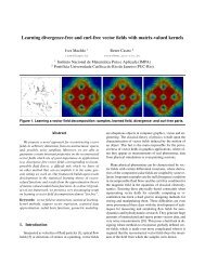
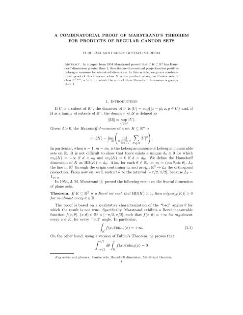
Abstract. In a paper from 1954 Marstrand proved that if K ⊂ R 2 has Hausdorff<br />
dimension greater than 1, then its one-dimensional projection has positive<br />
Lebesgue measure for almost-all directions. In this article, we give a combinatorial<br />
proof of this theorem when K is the product of regular Cantor sets of<br />
class C 1+α , α > 0, for which the sum of their Hausdorff dimension is greater<br />
than 1.<br />
1. Introduction<br />
If U is a subset of R n , the diameter of U is |U| = sup{|x−y|;x,y ∈ U} and, if<br />
U is a family of subsets of R n , the diameter of U is defined as<br />
‖U‖ = sup |U|.<br />
U∈U<br />
Given d > 0, the Hausdorff d-measure of a set K ⊆ R n is<br />
)<br />
∑<br />
m d (K) = lim |U| d<br />
ε→0<br />
(<br />
inf<br />
U covers K<br />
‖U‖ d 0 . We define the Hausdorff<br />
dimension of K as HD(K) = d 0 . Also, for each θ ∈ R, let v θ = (cosθ,sinθ), L θ<br />
the line in R 2 through the origin containing v θ and proj θ : R 2 → L θ the orthogonal<br />
projection. From now on, we’ll restrict θ to the interval [−π/2,π/2], because L θ =<br />
L θ+π .<br />
In 1954, J. M. Marstrand [4] proved the following result on the fractal dimension<br />
of plane sets.<br />
Theorem. If K ⊆ R 2 is a Borel set such that HD(K) > 1, then m(proj θ (K)) > 0<br />
for m-almost every θ ∈ R.<br />
The proof is based on a qualitative characterization of the “bad” angles θ for<br />
which the result is not true. Specifically, Marstrand exhibits a Borel measurable<br />
function f(x,θ), (x,θ) ∈ R 2 ×[−π/2,π/2], such that f(x,θ) = +∞ for m d -almost<br />
every x ∈ K, for every “bad” angle. In particular,<br />
∫<br />
f(x,θ)dm d (x) = +∞. (1.1)<br />
K<br />
U∈U<br />
On the other hand, using a version of Fubini’s Theorem, he proves that<br />
∫ π/2 ∫<br />
dθ f(x,θ)dm d (x) = 0<br />
−π/2<br />
K<br />
Key words and phrases. Cantor sets, Hausdorff dimension, Marstrand theorem.<br />
1<br />
.
2 YURI LIMA AND CARLOS GUSTAVO MOREIRA<br />
which, in view of (1.1), implies that<br />
m({θ ∈ [−π/2,π/2]; m(proj θ (K)) = 0}) = 0.<br />
These results are based on the analysis of rectangular densities of points.<br />
Many generalizationsand simpler proofs haveappeared since. One of them came<br />
in 1968 by R. Kaufman who gave a very short proof of Marstrand’s theorem using<br />
methods of potential theory. See [2] for his original proof and [5], [9] for further<br />
discussion.<br />
In this article, we prove a particular case of Marstrand’s Theorem.<br />
Theorem 1.1. If K 1 ,K 2 are regular Cantor sets of class C 1+α , α > 0, such that<br />
d = HD(K 1 ) + HD(K 2 ) > 1, then m(proj θ (K 1 ×K 2 )) > 0 for m-almost every<br />
θ ∈ R.<br />
The argument also works to show that the push-forward measure of the restriction<br />
of m d to K 1 ×K 2 , defined as µ θ = (proj θ ) ∗ (m d | K1×K 2<br />
), is absolutely continuous<br />
with respect to m, for m-almost every θ ∈ R. Denoting its Radon-Nykodim<br />
derivative by χ θ = dµ θ /dm, we also prove the following result.<br />
Theorem 1.2. χ θ is an L 2 function for m-almost every θ ∈ R.<br />
Remark1.3. Theorem1.2,asinthiswork,followsfrommostproofsofMarstrand’s<br />
theorem and, in particular, is not new as well.<br />
Our proof makes a study on the fibers proj θ −1 (v)∩(K 1 ×K 2 ), (θ,v) ∈ R×L θ ,<br />
and relies on two facts:<br />
(I) A regular Cantor set of Hausdorff dimension d is regular in the sense that the<br />
m d -measure of small portions of it has the same exponential behavior.<br />
(II)Thisenablesustoconcludethat, exceptforasmallsetofanglesθ ∈ R, thefibers<br />
proj θ −1 (v) ∩(K 1 ×K 2 ) are not concentrated in a thin region. As a consequence,<br />
K 1 ×K 2 projects into a set of positive Lebesgue measure.<br />
The idea of (II) is based on the work [6] of the second author. He proves that,<br />
if K 1 and K 2 are regular Cantor sets of class C 1+α , α > 0, and at least one<br />
of them is non-essentially affine (a technical condition), then the arithmetic sum<br />
K 1 +K 2 = {x 1 +x 2 ;x 1 ∈ K 1 ,x 2 ∈ K 2 } has the expected Hausdorff dimension:<br />
HD(K 1 +K 2 ) = min{1,HD(K 1 )+HD(K 2 )}.<br />
Marstrand’s Theorem for products of Cantor sets has many useful applications<br />
in dynamical systems. It is fundamental in certain results of dynamical bifurcations,<br />
namely homoclinic bifurcations in surfaces. For instance, in [10] it is used<br />
to show that hyperbolicity is not prevalent in homoclinic bifurcations associated to<br />
horseshoes with Hausdorff dimension larger than one; in [7] it is used to prove that<br />
stable intersections of regular Cantor sets are dense in the region where the sum of<br />
their Hausdorff dimensions is larger than one; in [8] to show that, for homoclinic<br />
bifurcations associated to horseshoes with Hausdorff dimension larger than one,<br />
typically there are open sets of parameters with positive Lebesgue density at the<br />
initial bifurcation parameter corresponding to persistent homoclinic tangencies.<br />
2. Regular Cantor sets of class C 1+α<br />
We say that K ⊂ R is a regular Cantor set of class C 1+α , α > 0, if:<br />
(i) there are disjoint compact intervals I 1 ,I 2 ,...,I r ⊆ [0,1] such that K ⊂<br />
I 1 ∪···∪I r and the boundary of each I i is contained in K;
MARSTRAND’S <strong>THEOREM</strong> <strong>FOR</strong> PRODUCTS <strong>OF</strong> CANTOR SETS 3<br />
(ii) there is a C 1+α expanding map ψ defined in a neighbourhood of I 1 ∪I 2 ∪<br />
···∪I r such that ψ(I i ) is the convex hull of a finite union of some intervals<br />
I j , satisfying:<br />
(ii.1) for each i ∈ {1,2,...,r} and n sufficiently big, ψ n (K ∩I i ) = K;<br />
(ii.2) K = ⋂ ψ −n (I 1 ∪I 2 ∪···∪I r ).<br />
n∈N<br />
The set {I 1 ,...,I r } is called a Markov partition of K. It defines an r×r matrix<br />
B = (b ij ) by<br />
b ij<br />
= 1, if ψ(I i ) ⊇ I j<br />
= 0, if ψ(I i )∩I j = ∅,<br />
which encodes the combinatorial properties of K. Given such matrix, consider the<br />
set Σ B = { θ = (θ 1 ,θ 2 ,...) ∈ {1,...,r} N ; b θiθ i+1<br />
= 1,∀i ≥ 1 } and the shift transformation<br />
σ : Σ B → Σ B given by σ(θ 1 ,θ 2 ,...) = (θ 2 ,θ 3 ,...).<br />
There is a natural homeomorphism between the pairs (K,ψ) and (Σ B ,σ). For<br />
each finite word a = (a 1 ,...,a n ) such that b aia i+1<br />
= 1, i = 1,...,n − 1, the<br />
intersection<br />
I a = I a1 ∩ψ −1 (I a2 )∩···∩ψ −(n−1) (I an )<br />
is a non-empty interval with diameter |I a | = |I an |/|(ψ n−1 ) ′ (x)| for some x ∈ I a ,<br />
which is exponentially small if n is large. Then, {h(θ)} = ⋂ n≥1 I (θ 1,...,θ n) defines a<br />
homeomorphism h : Σ B → K that commutes the diagram<br />
Σ B<br />
σ<br />
Σ B<br />
h<br />
h<br />
<br />
<br />
K ψ<br />
K<br />
Ifλ = sup{|ψ ′ (x)|;x ∈ I 1 ∪···∪I r } ∈ (1,+∞), then ∣ I(θ1,...,θ ∣<br />
n+1) ≥ λ −1·∣∣ I(θ1,...,θ ∣ n)<br />
and so, for ρ > 0 small and θ ∈ Σ B , there is a positive integer n = n(ρ,θ) such that<br />
ρ ≤ ∣ I(θ1,...,θ ∣ n) ≤ λρ.<br />
Definition 2.1. A ρ-decomposition of K is any finite set (K) ρ = {I 1 ,I 2 ,...,I r } of<br />
disjoint closed intervals of R, each one of them intersecting K, whose union covers<br />
K and such that<br />
ρ ≤ |I i | ≤ λρ, i = 1,2,...,r.<br />
Remark 2.2. Although ρ-decompositions are not unique, we use, for simplicity,<br />
the notation (K) ρ to denote any of them. We also use the same notation (K) ρ to<br />
denote the set ∪ I∈(K)ρ I ⊂ R and the distinction between these two situations will<br />
be clear throughout the text.<br />
EveryregularCantorset ofclass { C 1+α has a ρ-decomposition } for ρ > 0 small: by<br />
the compactness of K, the family I (θ1,...,θ n(ρ,θ))<br />
has a finite cover (in fact, it<br />
θ∈Σ B<br />
is only necessary for ψ to be of class C 1 ). Also, one can define ρ-decomposition for<br />
the product of two Cantor sets K 1 and K 2 , denoted by (K 1 ×K 2 ) ρ . Given ρ ≠ ρ ′<br />
and two decompositions (K 1 ×K 2 ) ρ ′ and (K 1 ×K 2 ) ρ , consider the partial order<br />
⋃ ⋃<br />
(K 1 ×K 2 ) ρ ′ ≺ (K 1 ×K 2 ) ρ ⇐⇒ ρ ′ < ρ and Q ′ ⊆<br />
Q ′ ∈(K 1×K 2) ρ ′<br />
Q∈(K 1×K 2) ρ<br />
Q.
4 YURI LIMA AND CARLOS GUSTAVO MOREIRA<br />
In this case, proj θ ((K 1 ×K 2 ) ρ ′) ⊆ proj θ ((K 1 ×K 2 ) ρ ) for any θ.<br />
A remarkable property of regular Cantor sets of class C 1+α , α > 0, is bounded<br />
distortion.<br />
Lemma 2.3. Let (K,ψ) be a regular Cantor set of class C 1+α , α > 0, and<br />
{I 1 ,...,I r } a Markov partition. Given δ > 0, there exists a constant C(δ) > 0,<br />
decreasing on δ, with the following property: if x,y ∈ K satisfy<br />
then<br />
(i) |ψ n (x)−ψ n (y)| < δ;<br />
(ii) The interval [ψ i (x),ψ i (y)] is contained in I 1 ∪···∪I r , for i = 0,...,n−1,<br />
In addition, C(δ) → 0 as δ → 0.<br />
e −C(δ) ≤ |(ψn ) ′ (x)|<br />
|(ψ n ) ′ (y)| ≤ eC(δ) .<br />
A direct consequence of bounded distortion is the required regularity of K, contained<br />
in the next result.<br />
Lemma 2.4. Let K be a regular Cantor set of class C 1+α , α > 0, and let d =<br />
HD(K). Then 0 < m d (K) < +∞. Moreover, there is c > 0 such that, for any<br />
x ∈ K and 0 ≤ r ≤ 1,<br />
c −1 ·r d ≤ m d (K ∩B r (x)) ≤ c·r d .<br />
ThesamehappensforproductsK 1 ×K 2 ofCantorsets(withoutlossofgenerality,<br />
considered with the box norm).<br />
Lemma 2.5. Let K 1 ,K 2 be regular Cantor sets of class C 1+α , α > 0, and let<br />
d = HD(K 1 )+HD(K 2 ). Then 0 < m d (K 1 ×K 2 ) < +∞. Moreover, there is c 1 > 0<br />
such that, for any x ∈ K 1 ×K 2 and 0 ≤ r ≤ 1,<br />
c 1<br />
−1 ·r d ≤ m d ((K 1 ×K 2 )∩B r (x)) ≤ c 1 ·r d .<br />
See chapter 4 of [9] for the proofs of these lemmas. In particular, if Q ∈ (K 1 ×<br />
K 2 ) ρ , there is x ∈ (K 1 ∪K 2 )∩Q such that B λ −1 ρ(x) ⊆ Q ⊆ B λρ (x) and so<br />
(<br />
c1 λ d) −1<br />
·ρ d ≤ m d ((K 1 ×K 2 )∩Q) ≤ c 1 λ d ·ρ d .<br />
Changing c 1 by c 1 λ d , we may also assume that<br />
c 1<br />
−1 ·ρ d ≤ m d ((K 1 ×K 2 )∩Q) ≤ c 1 ·ρ d ,<br />
which allows us to obtain estimates on the cardinality of ρ-decompositions.<br />
Lemma 2.6. Let K 1 ,K 2 be regular Cantor sets of class C 1+α , α > 0, and let<br />
d = HD(K 1 ) +HD(K 2 ). Then there is c 2 > 0 such that, for any ρ-decomposition<br />
(K 1 ×K 2 ) ρ , x ∈ K 1 ×K 2 and 0 ≤ r ≤ 1,<br />
( ) r<br />
#{Q ∈ (K 1 ×K 2 ) ρ ;Q ⊆ B r (x)} ≤ c 2 ·<br />
d·<br />
ρ<br />
In addition, c 2<br />
−1 ·ρ −d ≤ #(K 1 ×K 2 ) ρ ≤ c 2 ·ρ −d .
MARSTRAND’S <strong>THEOREM</strong> <strong>FOR</strong> PRODUCTS <strong>OF</strong> CANTOR SETS 5<br />
Proof. We have<br />
and then<br />
c 1 ·r d<br />
≥ m d ((K 1 ×K 2 )∩B r (x))<br />
∑<br />
≥ m d ((K 1 ×K 2 )∩Q)<br />
≥<br />
Q⊆B r(x)<br />
∑<br />
Q⊆B r(x)<br />
c 1<br />
−1 ·ρ d<br />
= #{Q ∈ (K 1 ×K 2 ) ρ ;Q ⊆ B r (x)}·c 1<br />
−1 ·ρ d<br />
( ) r<br />
#{Q ∈ (K 1 ×K 2 ) ρ ;Q ⊆ B r (x)} ≤ c 12 ·<br />
d·<br />
ρ<br />
On the other hand,<br />
∑<br />
∑<br />
m d (K 1 ×K 2 ) = m d ((K 1 ×K 2 )∩Q) ≤ c 1 ·ρ d ,<br />
Q∈(K 1×K 2) ρ Q∈(K 1×K 2) ρ<br />
implying that<br />
−1 #(K 1 ×K 2 ) ρ ≥ c 1 ·m d (K 1 ×K 2 )·ρ −d .<br />
Taking c 2 = max{c 2 1 , c 1 /m d (K 1 ×K 2 )}, we conclude the proof.<br />
□<br />
3. Proof of Theorem 1.1<br />
Given rectangles Q and ˜Q, let<br />
{<br />
}<br />
Θ Q, ˜Q<br />
= θ ∈ [−π/2,π/2];proj θ (Q)∩proj θ (˜Q) ≠ ∅ .<br />
Lemma 3.1. If Q, ˜Q ∈ (K 1 ×K 2 ) ρ and x ∈ (K 1 ×K 2 )∩Q,˜x ∈ (K 1 ×K 2 ) ∩ ˜Q,<br />
then<br />
( )<br />
ρ<br />
m Θ Q, ˜Q<br />
≤ 2πλ·<br />
d(x,˜x) ·<br />
Proof. Consider the figure.<br />
x<br />
θ |θ −ϕ 0|<br />
˜x<br />
L θ<br />
proj θ (˜x)<br />
θ<br />
proj θ (x)<br />
Since proj θ (Q) has diameter at most λρ, d(proj θ (x),proj θ (˜x)) ≤ 2λρ and then, by<br />
elementary geometry,<br />
sin(|θ −ϕ 0 |) = d(proj θ (x),proj θ (˜x))<br />
d(x,˜x)<br />
ρ<br />
≤ 2λ·<br />
d(x,˜x)<br />
ρ<br />
=⇒ |θ −ϕ 0 | ≤ πλ·<br />
d(x,˜x) ,
6 YURI LIMA AND CARLOS GUSTAVO MOREIRA<br />
because sin −1 y ≤ πy/2. As ϕ 0 is fixed, the lemma is proved.<br />
□<br />
Wepointoutthat, althoughingenuous,Lemma3.1expressesthecrucialproperty<br />
of transversality that makes the proof work, and all results related to Marstrand’s<br />
theorem use a similar idea in one way or another. See [11] where this tranversality<br />
condition is also exploited.<br />
Fixed a ρ-decomposition (K 1 ×K 2 ) ρ , let<br />
{<br />
N (K1×K 2) ρ<br />
(θ) = # (Q, ˜Q)<br />
}<br />
∈ (K 1 ×K 2 ) ρ ×(K 1 ×K 2 ) ρ ;proj θ (Q)∩proj θ (˜Q) ≠ ∅<br />
for each θ ∈ [−π/2,π/2] and<br />
E((K 1 ×K 2 ) ρ ) =<br />
∫ π/2<br />
−π/2<br />
N (K1×K 2) ρ<br />
(θ)dθ.<br />
Proposition 3.2. Let K 1 ,K 2 be regular Cantor sets of class C 1+α , α > 0, and let<br />
d = HD(K 1 ) +HD(K 2 ). Then there is c 3 > 0 such that, for any ρ-decomposition<br />
(K 1 ×K 2 ) ρ ,<br />
E((K 1 ×K 2 ) ρ ) ≤ c 3 ·ρ 1−2d .<br />
Proof. Let s 0 = ⌈ log 2 ρ −1⌉ and choose, for each Q ∈ (K 1 × K 2 ) ρ , a point x ∈<br />
(K 1 ×K 2 )∩Q. By a double counting and using Lemmas 2.6 and 3.1, we have<br />
∑ ( )<br />
E((K 1 ×K 2 ) ρ ) = Θ Q, ˜Q<br />
=<br />
Q, ˜Q∈(K 1×K 2) ρ<br />
m<br />
s 0<br />
∑<br />
s=1<br />
∑<br />
m<br />
Q, ˜Q∈(K 1 ×K 2 )ρ<br />
2 −s 1, c 3 = 2 d+1 πλc 22 ·∑s≥1 2s(1−d) < +∞ satisfies the required inequality.<br />
□<br />
This implies that, for each ε > 0, the upper bound<br />
N (K1×K 2) ρ<br />
(θ) ≤ c 3 ·ρ 1−2d<br />
ε<br />
(3.1)<br />
holds for every θ except for a set of measure at most ε. Letting c 4 = c 2<br />
−2 · c 3 −1 ,<br />
we will show that<br />
m(proj θ ((K 1 ×K 2 ) ρ )) ≥ c 4 ·ε (3.2)<br />
for every θ satisfying (3.1). For this, divide [−2,2] ⊆ L θ in ⌊4/ρ⌋ intervals J ρ 1 ,...,<br />
J ρ ⌊4/ρ⌋<br />
of equal lenght (at least ρ) and define<br />
s ρ,i = #{Q ∈ (K 1 ×K 2 ) ρ ; proj θ (x) ∈ J ρ i }, i = 1,...,⌊4/ρ⌋.
MARSTRAND’S <strong>THEOREM</strong> <strong>FOR</strong> PRODUCTS <strong>OF</strong> CANTOR SETS 7<br />
Then ∑ ⌊4/ρ⌋<br />
i=1<br />
s ρ,i = #(K 1 ×K 2 ) ρ and<br />
⌊4/ρ⌋<br />
∑<br />
i=1<br />
s ρ,i 2 ≤ N (K1×K 2) ρ<br />
(θ) ≤ c 3 ·ρ 1−2d ·ε −1 .<br />
Let S ρ = {1 ≤ i ≤ ⌊4/ρ⌋;s ρ,i > 0}. By Cauchy-Schwarz inequality,<br />
⎛ ⎞<br />
⎝ ∑<br />
2<br />
s ρ,i<br />
⎠<br />
i∈S ρ<br />
#S ρ ≥ ∑ ≥ c 2 −2 ·ρ −2d<br />
c 3 ·ρ 1−2d ·ε −1 = c 4 ·ε<br />
·<br />
ρ<br />
i∈S ρ<br />
s ρ,i<br />
2<br />
For each i ∈ S ρ , the interval J ρ i is contained in proj θ ((K 1 ×K 2 ) ρ ) and then<br />
which proves (3.2).<br />
m(proj θ ((K 1 ×K 2 ) ρ )) ≥ c 4 ·ε,<br />
Proof of Theorem 1.1. Fix a decreasing sequence<br />
(K 1 ×K 2 ) ρ1 ≻ (K 1 ×K 2 ) ρ2 ≻ ··· (3.3)<br />
of decompositions such that ρ n → 0 and, for each ε > 0, consider the sets<br />
G n ε = { θ ∈ [−π/2,π/2]; N (K1×K 2) ρn<br />
(θ) ≤ c 3 ·ρ n<br />
1−2d ·ε −1} , n ≥ 1.<br />
Then m([−π/2,π/2]\G n ε ) ≤ ε, and the same holds for the set<br />
G ε = ⋂ ∞⋃<br />
G l ε .<br />
n≥1<br />
If θ ∈ G ε , then<br />
l=n<br />
m(proj θ ((K 1 ×K 2 ) ρn )) ≥ c 4 ·ε, for infinitely many n,<br />
which implies that m(proj θ (K 1 ×K 2 )) ≥ c 4 · ε. Finally, the set G = ∪ n≥1 G 1/n<br />
satisfies m([−π/2,π/2]\G) = 0 and m(proj θ (K 1 ×K 2 )) > 0, for any θ ∈ G. □<br />
4. Proof of Theorem 1.2<br />
Given any X ⊂ K 1 × K 2 , let (X) ρ be the restriction of the ρ-decomposition<br />
(K 1 × K 2 ) ρ to those rectangles which intersect X. As done in Section 3, we’ll<br />
obtain estimates on the cardinality of (X) ρ . Being a subset of K 1 ×K 2 , the upper<br />
estimates from Lemma 2.6 also hold for X. The lower estimate is given by<br />
Lemma 4.1. Let X be a subset of K 1 ×K 2 such that m d (X) > 0. Then there is<br />
c 6 = c 6 (X) > 0 such that, for any ρ-decomposition (K 1 ×K 2 ) ρ and 0 ≤ r ≤ 1,<br />
c 6 ·ρ −d ≤ #(X) ρ ≤ c 2 ·ρ −d .<br />
Proof. As m d (X) < +∞, there exists c 5 = c 5 (X) > 0 (see Theorem 5.6 of [1]) such<br />
that<br />
m d (X ∩B r (x)) ≤ c 5 ·r d , for all x ∈ X and 0 ≤ r ≤ 1,<br />
and then<br />
m d (X) = ∑<br />
m d (X ∩Q) ≤ ∑<br />
c 5 ·(λρ) d = ( c 5 ·λ d)·ρ d ·#(X) ρ .<br />
Q∈(X) ρ Q∈(X) ρ<br />
Just take c 6 = c 5<br />
−1 ·λ −d ·m d (X).<br />
□
8 YURI LIMA AND CARLOS GUSTAVO MOREIRA<br />
Proposition 4.2. The measure µ θ = (proj θ ) ∗ (m d | K1×K 2<br />
) is absolutely continuous<br />
with respect to m, for m-almost every θ ∈ R.<br />
Proof. Note that the implication<br />
X ⊂ K 1 ×K 2 , m d (X) > 0 =⇒ m(proj θ (X)) > 0 (4.1)<br />
is sufficient for the required absolute continuity. In fact, if Y ⊂ L θ satisfies m(Y) =<br />
0, then<br />
µ θ (Y) = m d (X) = 0,<br />
whereX = proj θ −1 (Y). Otherwise,by(4.1)wewouldhavem(Y) = m(proj θ (X)) ><br />
0, contradicting the assumption.<br />
We prove that (4.1) holds for every θ ∈ G, where G is the set defined in the<br />
proof of Theorem 1.1. The argument is the same made after Proposition 3.2: as,<br />
by the previous lemma, #(X) ρ has lower and upper estimates depending only on<br />
X and ρ, we obtain that<br />
m(proj θ ((X) ρn )) ≥ c 3<br />
−1 ·c 62 ·ε, for infinitely many n,<br />
and then m(proj θ (X)) > 0.<br />
Let χ θ = dµ θ /dm. In principle, this is a L 1 function. We prove that it is a L 2<br />
function, for every θ ∈ G.<br />
Proof of Theorem 2. Let θ ∈ G 1/m , for some m ∈ N. Then<br />
N (K1×K 2) ρn<br />
(θ) ≤ c 3 ·ρ n<br />
1−2d ·m, for infinitely many n. (4.2)<br />
For each of these n, consider the partition P n = {J ρn<br />
1 ,...,Jρn ⌊4/ρ n⌋ } of [−2,2] ⊂ L θ<br />
into intervals of equal length and let χ θ,n be the expectation of χ θ with respect<br />
to P n . As ρ n → 0, the sequence of functions (χ θ,n ) n∈N converges pointwise to χ θ .<br />
By Fatou’s Lemma, we’re done if we prove that each χ θ,n is L 2 and its L 2 -norm<br />
‖χ θ,n ‖ 2<br />
is bounded above by a constant independent of n.<br />
By definition,<br />
and then<br />
µ θ (J ρn<br />
i<br />
) = m d<br />
(<br />
(projθ ) −1 (J ρn<br />
i<br />
) ) ≤ s ρn,i ·c 1 ·ρ n d , i = 1,2,...,⌊4/ρ n ⌋,<br />
implying that<br />
i )<br />
|J ρn<br />
i |<br />
χ θ,n (x) = µ θ(J ρn<br />
‖χ θ,n ‖ 2 2<br />
=<br />
=<br />
≤<br />
∫<br />
≤ c 1 ·s ρn,i ·ρ n<br />
d<br />
|J ρn<br />
i |<br />
L θ<br />
|χ θ,n | 2 dm<br />
⌊4/ρ<br />
∑ n⌋<br />
i=1<br />
⌊4/ρ<br />
∑ n⌋<br />
i=1<br />
∫<br />
J ρn<br />
i<br />
|J ρn<br />
i |·<br />
|χ θ,n | 2 dm<br />
⌊4/ρ<br />
∑ n⌋<br />
2d−1 ≤ c 12 ·ρ n ·<br />
, ∀x ∈ J ρn<br />
i ,<br />
(<br />
c1 ·s ρn,i ·ρ n<br />
d<br />
i=1<br />
|J ρn<br />
i |<br />
s ρn,i 2<br />
≤ c 12 ·ρ n<br />
2d−1 ·N (K1×K 2) ρn<br />
(θ).<br />
) 2<br />
□
MARSTRAND’S <strong>THEOREM</strong> <strong>FOR</strong> PRODUCTS <strong>OF</strong> CANTOR SETS 9<br />
In view of (4.2), this last expression is bounded above by<br />
(<br />
c12 ·ρ n<br />
2d−1 )·(c 3 ·ρ n<br />
1−2d ·m ) = c 12 ·c 3 ·m,<br />
which is a constant independent of n.<br />
□<br />
5. Concluding remarks<br />
The proofs of Theorems 1.1 and 1.2 work not just for the case of products of<br />
regular Cantor sets, but in greater generality, whenever K ⊂ R 2 is a Borel set for<br />
which there is a constant c > 0 such that, for any x ∈ K and 0 ≤ r ≤ 1,<br />
c −1 ·r d ≤ m d (K ∩B r (x)) ≤ c·r d ,<br />
since this alone implies the existence of ρ-decompositions for K.<br />
The good feature of the proof is that the discretization idea may be applied<br />
to other contexts. For example, we prove in [3] a Marstrand type theorem in an<br />
arithmetical context.<br />
Acknowledgments<br />
The authors are thankful to IMPA for the excellent ambient during the preparation<br />
of this manuscript. The authors are also grateful to Carlos Matheus for<br />
carefully reading the preliminary version of this work and the anonymous referee<br />
for many useful and detailed recommendations. This work was financially supported<br />
by CNPq-Brazil and Faperj-Brazil.<br />
References<br />
1. K. Falconer, The geometry of fractal sets, Cambridge Tracts in Mathematics, Cambridge<br />
(1986).<br />
2. R. Kaufman, On Hausdorff dimension of projections, Mathematika 15 (1968), 153–155.<br />
3. Y. Lima and C.G. Moreira, A Marstrand theorem for subsets of integers, available at<br />
http://arxiv.org/abs/1011.0672.<br />
4. J.M. Marstrand, Some fundamental geometrical properties of plane sets of fractional dimensions,<br />
Proceedings of the London Mathematical Society 3 (1954), vol. 4, 257–302.<br />
5. P. Mattila, Hausdorff dimension, projections, and the Fourier transform, Publ. Mat. 48<br />
(2004), no. 1, 3–48.<br />
6. C.G. Moreira, A dimension formula for arithmetic sums of regular Cantor sets, to appear.<br />
7. C.G. Moreira and J.C. Yoccoz, Stable Intersections of Cantor Sets with Large Hausdorff<br />
Dimension, Annals of Mathematics 154 (2001), 45–96.<br />
8. C.G. Moreira and J.C. Yoccoz, Tangences homoclines stables pour des ensembles hyperboliques<br />
de grande dimension fractale, Annales scientifiques de l’ENS 43, fascicule 1 (2010).<br />
9. J. Palis and F. Takens, Hyperbolicity and sensitive chaotic dynamics at homoclinic bifurcations,<br />
Cambridge studies in advanced mathematics, Cambridge (1993).<br />
10. J. Palis and J.C. Yoccoz, On the Arithmetic Sum of Regular Cantor Sets, Annales de<br />
l’Inst. Henri Poincar, Analyse Non Lineaire 14 (1997), 439–456.<br />
11. M. Rams, Exceptional parameters for iterated function systems with overlaps, Period. Math.<br />
Hungar. 37 (1998), no. 1-3, 111–119.<br />
12. M. Rams, Packing dimension estimation for exceptional parameters, Israel J. Math. 130<br />
(2002), 125–144.<br />
Instituto Nacional de Matemática Pura e Aplicada, Estrada Dona Castorina 110,<br />
22460-320, Rio de Janeiro, Brasil.<br />
E-mail address: yurilima@impa.br<br />
Instituto Nacional de Matemática Pura e Aplicada, Estrada Dona Castorina 110,<br />
22460-320, Rio de Janeiro, Brasil.<br />
E-mail address: gugu@impa.br