Reference Guide & Formula Sheet for Physics - 2006 Version

Reference Guide & Formula Sheet for Physics 

Dr. Mitchell A. Hoselton Physics − Douglas C. Giancoli Page 1 of 16 

Chapter 01. – Units, Unit Conversion, Symbols Chapter 01. – continued 

Units are important. You will learn the names of lots of 

units this year. Each unit has a standard one or twoletter 

abbreviation. You must learn the abbreviations 

and use them. Start with these few. 

(The unit of time is the second = s) 

(The unit of distance or displacement is the meter = m) 

(The unit of velocity is meters per second = m/s) 

(The unit of acceleration is meters per second squared = m/s 2 ) 

Symbols are important. They stand in for known and 

unknown quantities in the equations you will derive to 

solve Physics problems. Many of these symbols are 

considered so standard that everyone everywhere uses 

the same symbol. This actually simplifies matters is 

many cases. We will use the standard symbols 

whenever possible. You will have to learn these as we 

move along. Start with these few. 

(The symbol of time is t) 

(The symbol of distance is d) 

(The symbol of speed is v or s) 

(The symbol of displacement is d or r or s) 

(The symbol of velocity is v) 

(The symbol of acceleration is a) 

Subscripts are important. Subscripts add essential 

information that must be taken into account. For 

example, v 0 usually indicates the velocity at time zero, 

while v i and v f usually indicate the initial and final 

velocities, and v AVE is the average velocity. These are 

all different velocities. Always read the subscripts. 

Time is important. Time started 14 billion years ago 

when the universe appeared. We will not be studying 

processes that began at the beginning of time. All times 

that we measure are therefore time intervals, or time 

differences, if you like. For us time zero always means 

that time when the clock started. And time t always 

means the time interval since the clock started. In light 

of this fact, is it never wrong to replace t with a ∆t in 

any equation. If the time interval does not start at time 

zero on the clock, then the time must be written as ∆t. 

Standard Units: The standard units we use are known mi 5280 ft 

35.0 × × 

as SI units. For now, learn these first few. 

hr 1 mi 

Measure of length meters = m 

1hr 

× × 

Measure of area meters 2 = m 2 = m×m 

60 min 

Measure of volume meters 3 = m 3 = m×m×m 

Measure of time seconds = s 

Measure of velocity meters per second = m/s 

Measure of acceleration meters per second 2 = m/s 2 

Error and Precision are not the same thing. Error tells 

us how far the measurement is from the true answer. We 

will usually report error as Percent Error. 

%Error=100%×|Measured−True|/True 

Precision tells us only how consistently a given 

measuring device can measure values ACCORDING TO 

ITS MANUFACTURER’S SPECIFICATION. 

Precision is a measure of the reproducibility and 

consistency of the results. The measurements can be 

very consistent and still be consistently wrong, however. 

Typically, the specification for the precision of a device 

might be reported something like one of the following, 

±0.002 

±1% 

3½ digits 

Fine precision is no guarantee of high accuracy, 

however. Usually the two go together, but sometimes, 

probably by mistake, they do not. (Hubble Telescope!) 

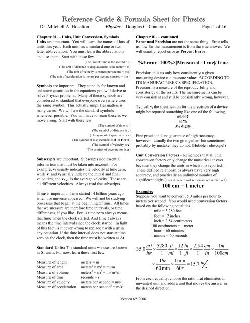
Unit Conversion Factors – Remember that all unit 

conversion factors only change the numerical answer 

because they change the units in which it is reported. 

These defined relationships always have very high 

accuracy, and practically an unlimited number of 

significant digits (even if the terminal zeroes are not written out). 

100 cm = 1 meter 

Example: 

Suppose you want to convert 35.0 miles per hour to 

meters per second. You would need conversion factors 

based on the following equalities. 

1 mile = 5,280 feet 

1 foot = 12 inches 

1 inch = 2.54 centimeters 

100 centimeters = 1 meter 

1 hour = 60 minutes 

1 minute = 60 seconds 

12 in 2.54 cm 1m 

× × 

1 ft 1 in 100cm 

1min 

= 15.7 m 

60s 

s 

From each equality, choose the ratio that eliminates an 

unwanted unit and adds a unit that moves the answer in 

the desired direction. 

Version 6/5/2006



Chapter 02. – Motion Along one Axis 

Physical quantities for which the direction of their 

motion or action is an important characteristic must be 

treated mathematically using vectors, not simple 

numerical values. Quantities that do not require 

directional information are called scalars. We begin our 

study of vectors by studying motion in one direction. 

This type of vector behaves much like a scalar quantity; 

only the notation is a little different at this point. 

Vectors are symbolized with very bold letters. The 

most important quantities in this section are the 

instantaneous quantities listed here. 

Instantaneous position: 

Instantaneous position at time zero: x 0 

Instantaneous velocity: 

Instantaneous velocity at time zero: v 0 

Instantaneous acceleration: 

x 

v 

a 

(for now, acceleration is assumed to be constant.) 

Chapter 02. – continued 

With the definition of distance in hand we can define the 

scalar quantity known at the average speed. 

v AVG = average speed = distance/∆time = d/∆t 

Where ∆t is the time interval between the moment when 

the object was at the initial position and the moment 

when it was at the final position. The time interval is 

often writing simply as t, but this is only true if the time 

interval begins at the moment when the clock reads zero. 

(Think of the clock as a stopwatch.) 

With the definition of the displacement in hand we can 

define the vector quantity known as the average velocity 

v AVG = average velocity = displacement/∆time = d/∆t 

Instantaneous Position – x – the position of a moving 

object at one moment in time; also known as an instant 

of time. Position is always assumed to be instantaneous. 

Before we can rigorously define what we mean by 

instantaneous, we need to define some simpler 

quantities. The first of these are distance and 

displacement. In one dimension these might have the 

same numeric value. 

d = distance = odometer reading 

If the object starts at x 0 and moves back and forth 

before settling at its final position, x, then the distance 

could be much longer than the shortest path between the 

starting and ending points. On the other hand, the 

minimum distance is closely related to the displacement. 

d MIN = |x − x 0 | = |x 0 − x| = |d| 

The minimum distance does not include information 

about the direction of travel; that is the meaning of those 

absolute value markers. The starting and ending 

positions are x 0 and x, but the scalar quantity called 

“minimum distance” does not care which is which. 

Subtraction in either order is permitted. 

d = displacement = x − x 0 = d 

The vector quantity called “displacement”, on the other 

hand, must be calculated as the final position vector 

minus the initial position vector. That result always 

gives us the minimum distance and the direction of the 

motion. For motion along the x-axis, as one example, a 

positive displacement indicates motion to the right. A 

negative displacement indicates motion to the left. 

Version 6/5/2006 

Instantaneous Velocity – v – is average velocity over 

an infinitesimal displacement in an infinitesimal time 

interval. It is the velocity at one instant. As a practical 

matter it is usually good enough to measure the average 

velocity over a short displacement in a brief time interval 

and then take the ratio of those two measurements to 

estimate the instantaneous velocity. 

Constant-Acceleration Linear Motion 

Once our final definitions for instantaneous position and 

instantaneous velocity are completed, the following 

equations of motion apply to all systems that have a 

constant acceleration. (When the acceleration is constant, the 

instantaneous and average accelerations have the same magnitude and 

direction.) 

v = v 0 + a•t 

no x 

(x − x 0 ) = v 0 •t + ½•a•t² no v 

v² = v 0 ² + 2•a•(x − x 0 ) no t 

(x − x 0 ) = ½•(v 0 + v)•t no a 

(x − x 0 ) = v•t − ½•a•t² no v ο 

Average velocity can be obtained from the initial and 

final instantaneous velocities, if and only if the 

acceleration is constant. 

v AVE 

v + v 

= 

2 

0 

= 

average velocity




Constant Acceleration is rare in nature but common in 

the problems we will be working. Constant acceleration 

gives the equations of motion their simplest form and 

makes them easier to solve. Gravity provides a ready 

source of objects moving with constant acceleration. 

Strictly speaking, we cannot define average acceleration 

until we have a definition for instantaneous velocity. 

Then the average acceleration is 

a AVG = average acceleration 

= velocity change/∆time = ∆v/∆t 

When the acceleration is constant, the instantaneous and 

average acceleration have the same magnitude and 

direction. Since the instantaneous acceleration is the 

same at all moments, the average acceleration must have 

the same magnitude and direction. 

One dimensional vectors 

To this point, we’ve used only vectors that behave 

exactly like signed numerical values, where the sign 

indicates the direction along the axis of motion. 

Vectors can also be thought of as arrows with pointed 

ends showing the direction of the motion. We could 

even use these arrows to describe the one-dimensional 

vectors discussed in this chapter. 

In the next chapter, where objects are free to move in 

two dimensions, we will use the arrow representation 

first. There is also a method that allows us to reuse the 

vector concepts from this chapter; the signed numbers. 

We will separate the vectors into what are call their 

components. Components are independent onedimensional 

sub-sets of the motion. 

Chapter 03. – 

Components of a Vector and Vector Addition 

V = v ∠θ = 34.0 m/s ∠48.0° 

v x = v cos θ = 34 m/s•(cos 48°) = 22.8 m/s 

v y = v sin θ = 34 m/s•(sin 48°) = 25.3 m/s 

V = v x i + v y j = 22.8 i + 25.3 j m/s 

W = w ∠θ = 52.0 m/s ∠113.0° 

w x = w cos θ = 52 m/s•(cos 113°) = −20.3 m/s 

w y = w sin θ = 52 m/s•(sin 113°) = 47.9 m/s 

w = w x i + w y j = −20.3 i + 47.9 j m/s 


V + w = (22.8−20.3) i + (25.3+47.9) j m/s 

V + w = 2.5 i + 73.2 j m/s = w + V 

V − w = (22.8−(−20.3)) i + (25.3−47.9) j m/s 

= 43.1 i − 22.6 j m/s 

w − V = (−20.3−22.8) i + (47.9−25.3) j m/s 

= −43.1 i + 22.6 j m/s 

V − w and w − V, point in opposite directions and 

both are perpendicular to V + w = w + V. 

Projectile Motion – working with components 

Horizontal position: x−x ο = v x •t 

Vertical position: y−y ο = v y0 •t − ½•g•t² 

Horizontal velocity: v x = v 0 cos θ 

Vertical velocity: v y = v 0 sin θ – gt 2 

Horizontal acceleration: a x = 0 

Vertical acceleration: a y = −g = constant 


Newton’s First Law – Law of Inertia. Forces make 

objects move. No force means no change in the motion. 

Newton's Second Law – Forces cause acceleration. 

F net 

= ΣF Ext = m sys •a sys 

Newton’s Third Law – Forces are created in pairs. 

Weight = W = m•g 

g = 9.80m/s² near the surface of the Earth 

= 9.795 m/s² in Fort Worth, TX 

Friction Force = F F = µ•F N 

If the object is not moving, you are dealing with static 

friction and it can have any value from zero up to µ S 

F N 

If the object is sliding, then you are dealing with kinetic 

friction and it will be constant and equal to µ K 

F N 

Free-Body Diagram – Show all the forces acting on and 

object. Components must be dashed to distinguish them 

from forces. You cannot use a force and its components 

in the same problem. 





Uniform Circular Motion - Centripetal Acceleration 

Uniform Circular Motion – Period, Frequency and V 

T 

1 

= 

f 

Centripetal Force 

Minimum Speed at the top of a Vertical Loop 

rg v = 

Circular Unbanked Track – Car Rounding a Curve. 

2 

mv 

F = µ mg = = 

r 

C 

ma R 

Banked Circular Track 

v 2 = r•g•tan θ, without friction 

Universal Gravitation – Conservative Force 

m m 

F = G 

r 

1 2 

2 

where G = 6.67 ×10 −11 N•m² / kg² = 6.67 E−11 N•m² / kg² 


and 

v 

= 

r 

a R 

2 

f 

mv 

r 

1 

= 

T 

and v = 

2 

2 

F C 

= 

= mω 

r 

2πr 

T 

Work done by a constant force = F•D•cos θ 

Where D is the displacement of the mass and 

θ is the angle between F and D. unit : N•m = J 

Work done by a varying force 

On a graph of Force vs displacement the work is the 

area between the curve and the x-axis. Later on we 

will evaluate this are by taking the anti-derivative of 

the function that describes the force in terms of 

position. 

Mechanical Energy –Kinetic Energy 

KE Linear = K = ½•m•v² 

Chapter 06 – continued 

Mechanical Energy – The Work-Energy Theorem 

The net work done on a body equals the change in 

the kinetic energy of the body. 

W net = ∆KE = KE f − KE i 

= ½•m•v f ² − ½•m•v i ² 

Mechanical Energy – Gravitational Potential Energy 

PE Grav = PE g = m•g•h 

= m•g•y 

Hooke's Law – a non-constant force 

F = −k•x 

x = displacement from equilibrium 

k = the spring constant 

= proportionality constant between 

the restoring force and the 

displacement. 

Potential Energy of a spring – Conservative Force 

Work done on a spring = PE = W = ½•k•x² 

Power = rate of work done, unit = J/s = W = watts 

Work Fd 

average power = P = = = Fv 

∆time 

∆t 


Linear Momentum 

momentum = p = m•v = mass • velocity 

Newton's Second Law 

F 

= ΣF 

∆p 

mv − mv 

= = 

∆t 

∆t 

m( v − v ) 

0 

= 

∆t 

0 

= 

net Ext 

Impulse = Change in Momentum 

F•∆t = ∆p = ∆(m•v) 

ma 

Conservation of Momentum in Collisions 

m A •v A + m B •v B = m A •v A ’ + m B •v B ’ 

Sum of Momenta before the Collision 

Sum of Momenta after the Collision 

Center of Mass – point masses on a line (x only), on a 

plane (x and y only), or filling space (x, y, and z) 

x cm = Σ(m i •x i ) / M total 

y cm = Σ(m i •y i ) / M total 

z cm = Σ(m i •z i ) / M total 





Angular Distance – Radian measure 

θ = arc length/radius = l/r = s / r 

360º = 2π radians 

Angular Speed vs. Linear Speed 

Linear speed = v = r•ω = radius • angular speed 

Constant Angular-Acceleration in Circular Motion 

ω = ω ο + α•t 

no θ 

θ−θ ο = ω ο •t + ½•α•t² no ω 

ω 2 2 

= ω ο + 2•α•(θ−θο ) no t 

θ−θ ο = ½•(ω ο + ω)•t no α 

θ−θ ο = ω•t - ½•α•t² no ω ο 

Torque = τ = F•L•sin θ 

Where θ is the angle between F and L; unit: N•m 


Elasticity; Stress and Strain 

(Assumes objects stretch according to Hooke’s Law as long as 

they 

are not stretched passed the proportional limit.) 

For tensile stress 

F = k•∆L = (EA/L 0 )•∆L 

F = applied force 

E = elastic (or Young’s) modulus 

A = cross-sectional area – 

perpendicular to the force 

L 0 = the original length 

∆L = change in the length 

∆L/L 0 = (1/E)•(F/A) 

strain = (1/E)•(stress) 

E = (stress / strain) 

Newton's Second Law for Rotation 

torque = τ = I•α 

moment of inertia = I CM = m•r² (for a point mass) 

Rotational Kinetic Energy (See LEM on last page) 

KE rotational = ½•I•ω 2 = ½•I• (v / r) 2 

KE rolling w/o slipping = ½•m•v 2 + ½•I•ω 2 

Moment of Inertia – I CM 

point mass I CM = m•r 2 

cylindrical hoop I CM = m•r 2 

solid cylinder or disk I CM = ½ m•r 2 

solid sphere I CM = 2 / 5 m•r 2 

hollow sphere I CM = ⅔ m•r 2 

thin rod (center) I CM = 1 / 12 m•L 2 

When the thin rod is rotated about its end rather than 

about is center of mass, the moment of inertia becomes 

thin rod (end) I End = ⅓ m•L 2 

Angular Momentum = L = I•ω = m•v•r•sin θ 

Angular Impulse equals CHANGE IN Angular 

Momentum 

∆L = τ Average •∆t = ∆(I•ω) 

Compressive stress is the exact opposite of tensile 

stress. Objects are compressed rather than 

stretched. As for springs the equations are the same 

for both tensile and compressive stress and the same 

elastic modulus is used for both calculations. 

∆L/L 0 = −(1/E)•(F/A) 

strain = − (1/E)•(stress) 

E = − (stress / strain) 

There is a negative sign because the length 

decreases as the force increases (∆L is negative). 

Shear stress is the application of two forces that distort 

an object (like deforming a rectangle into a parallelogram). 

The forces are equal and opposite (parallel, but not 

oriented to directly oppose each other). (A second pair of 

matched forces is also required to maintain equilibrium while the 

stress is applied.) 

∆L /L 0 = (1/G)•(F/A) 

strain = (1/G)•(stress) 

G = (stress / strain) 

G = shear modulus 

A = area – Parallel to the force. 

L 0 = original length of object 

∆L = change in length due to force 

Note that ∆L is perpendicular to L 0 . 





Bulk Stress - When the force is applied uniformly all 

over an object, we expect its volume to shrink. When 

applied this way, the ratio of force to area is called 

“pressure”, and ∆P is the change in pressure that induces 

a corresponding change in the volume. 

∆V/V 0 = −(1/B)•(∆P) 

strain = −(1/B)•(stress) 

B = −(stress / strain) 

B = bulk modulus 

V 0 = initial volume of the material 

∆V = Change in the volume 

∆P = change in pressure 

The minus sign indicates that the volume decreases 

when the pressure increases. When ∆P is positive, ∆V is 

negative, and vice versa. One of the two is always 

negative. 


Pressure under Water (or immersed in any liquid) 

P = ρ•g•h 

Density = mass / volume 

ρ = 

P = Pressure at depth 

h = depth below the surface 

ρ = density of the fluid 

m 

V 

3 

( unit : kg / m ) 

Buoyant Force - Buoyancy 

F B = ρ•V•g 

= m Displaced fluid •g 

= weight Displaced fluid 

ρ = density of the fluid 

V = volume of fluid displaced 

Continuity of Fluid Flow 

Q Volume Flow Rate = A in •v in = A out •v out 

A = Cross-sectional Area 

v = velocity of the fluid 


Poiseuille's Equation (Laminar flow in horizontal tubular pipes.) 

Q = volume flow rate of fluid = m 3 /s 

Q = (π•r 4 ) ∆P / (8•η•L) 

r = inside radius of pipe = m 

∆P = P 1 – P 2 = Pressure change = Pa 

η = coefficient of viscosity = Pa•s 

L = length of pipe = m 

Bernoulli's Equation 

P + ρ•g•h + ½•ρ•v ² = constant 

Q Volume Flow Rate = A 1 •v 1 = A 2 •v 2 = constant 


Period of Simple Harmonic Motion – Ideal Spring 

also f = 1/ T 

where k = spring constant, and m is the mass. 

Simple Pendulum 

T = 

2π 

T = 2π 

also f = 1/ T 

where L is the length of the pendulum and g is 

the local acceleration due to gravity. 

Velocity of Periodic Waves 

f = 1 / T 

v = f •λ = λ/Τ 

where T = the period of the wave 

Speed of a Wave on a String 

L 

g 

m 

k 

mv 2 

T = ; therefore, v = 

L 

T 

m/L 

T = tension in string 

m = mass of string 

L = length of string 

Sinusoidal motion 

x = A•cos(ω•t) = A•cos(2•π•f •t) 

ω = angular frequency 

f = frequency 





Doppler Effect 

f 

v o 

= velocity of observer: 

v s 

= velocity of source 

v SOUND = 343 m/s 

Decibel Scale 

dB (Decibel level) = 10 log ( I / I o 

) 

I = intensity of sound 

I o 

= intensity of softest audible sound 


Ideal Gas Law 

′ = 

Toward 

Away 

Toward 

Away 

P•V = n•R•T 

n = # of moles of gas 

R = gas law constant 

= 8.31 J/mol•K. 

Thermal Expansion of Solids 

Linear: ∆L = L o 

•α•∆T 

Volume: ∆V = V o 

•β•∆T 


Heating a Solid, Liquid or Gas 

Q = m•c•∆T 

f 

343 ± 

343 

m 

v 

v 

(no phase changes!) 

Q = the heat added 

c = specific heat. 

∆T = temperature change, K or ºC 

o 

s 


First Law of Thermodynamics 

∆U = Q Net + W Net 

Change in Internal Energy of a system = 

+Net Heat added to the system 

+Net Work done on the system 

Work done on a gas or by a gas 

W = P•∆V 

2 nd Law of Thermodynamics 

The change in internal energy of a system is 

∆U = Q Added + W DoneOn – Q lost – W DoneBy 

Maximum Efficiency of a Heat Engine (Carnot Cycle) 

Tc 

% Eff = (1 − ) ⋅100% 

T 

Efficiency = Work out / Energy in 

(Temperatures in Kelvin) 

Mechanical Advantage = force out / force in 

M.A. = F out / F in 

Entropy change at constant T 

∆S = Q / T 

(Applies to phase changes only: melting, boiling, freezing, etc) 


Coulomb's Law 

h 

F = k 

k = = 8.85× 

10 

4πε 

q 

1 + 9 

o 

1 2 

2 

r 

q 

N ⋅ m 

2 

C 

2 

N ⋅ m 

≈ 9E9 

2 

C 

2 

Heat required for a Phase Change 

Q = m•L 

m = mass of material 

L = Latent Heat of phase change 

Flow of Heat through a Solid 

∆Q / ∆t = k•A•∆T / L 

k = thermal conductivity 

A = area of solid 

∆T = Temperature difference 

L = thickness of solid 

Electric Field around a point charge 

E = k 

1 + 9 

k = = 8.85× 

10 

4πε 

o 

r 

q 

2 

N ⋅ m 

2 

C 

2 

N ⋅ m 

≈ 9E9 

2 

C 

2 





Capacitors and Capacitance 

Q c = C•V c 

Q c = charge on capacitor 

(The unit of electric charge is the coulomb = C) 

C = capacitance of the capacitor 

(The unit of capacitance is the farad = F = C/V) 

V c = voltage across the plates 

(The unit of voltage is the volt = V = J/C) 


Resistor Combinations 

SERIES 

R eq = R 1 + R 2 + R 3 +. . . 

1 

R 

eq 

= 

1 

R 

1 

+ 

1 

R 

PARALLEL 

2 

+ K + 

1 

R 

n 

= 

n 

∑ 

i= 

1 

1 

R 

i 

Potential Energy stored in a Capacitor 

P = ½•C•V² 


Ohm's Law 

V = I•R 

V = voltage across the resistor 

(The unit of voltage is the volt = V = J/C) 

I = current through the resistor 

(The unit of current is the ampere = A = C/s) 

R = resistance of the resistor 

(The unit of resistance is the ohm = Ω = V/A) 

Resistance of a resistor (or any resistive material) 

R = ρ•L / A x 

ρ = resistivity of the material 

(The unit of resistivity is the ohm•meter = Ω•m) 

L = length of the material 

(The unit of length is the meter = m) 

A x = cross-sectional area of the 

Material or resistor 

(The unit of cross-sectional area is meter 2 = m 2 ) 

Electric Power (The unit of power is the watt = W = J/s) 

P = I²•R 

P = V ² / R 

P = I•V 

Capacitor Combinations 

SERIES 

1 

= 

1 

Kirchhoff’s Laws 

1 

+ 

C 

1 

+ K + 

C 

PARALLEL 

C eq = C 1 + C 2 + C 3 + … 

Node Rule: Σ node I i = 0 

Loop Rule: Σ loop ∆V i = 0 

Capacitance, C, of a Capacitor 

C = κ•εo•A / d 

n 1 

= ∑ 

i = 

C 

1 

C C 

eq 

1 

2 

n 

κ = dielectric constant 

A = area of plates 

d = distance between plates 

ε o 

= 8.85 10 −12 ) F/m 

(Capital “C” is also used as the abbreviation for the unit of electric 

charge; the coulomb = C. Do not confuse the two uses of capital “C”. 

The unit of capacitance is the farad = F. The capital “F” is frequently 

used as the symbol for force. Do not confuse the two used of the 

capital “F”.) 

RC Circuit formula (Charging with one battery, one 

resistor and one capacitor) 

V Battery 

− V capacitor − I•R = 0 

RC Circuits (Charging) - R•C = τ = time constant 

V c = V MAX •[1 - e −t/RC ] 

But V c − I•R = 0 (from Ohm’s Law), therefore, 

I = (V MAX /R)•e −t/RC 

= I MAX•e −t/RC 

And Q c = CV c (from the definition of capacitance), so 

Q c = C•V MAX •[1 − e −t/RC ] 

= Q MAX •[1 − e −t/RC ] 

i 





RC Circuits (Discharging) - R•C = τ = time constant 

V c = V MAX •e −t/RC 

But V c − I•R = 0 (from Ohm’s Law), therefore, 

I = (V MAX /R)•e −t/RC 

= I MAX•e −t/RC 

And Q c = CV c (from the definition of capacitance), so 

Q c =C•V MAX •e −t/RC 

=Q MAX •e −t/RC 


Magnetic Field around a wire 

Magnetic Flux 

B 

Φ = B•A•cos θ 

Force caused by a magnetic field acting on a 

moving charge 

F = q•v•B•sin θ 


Induced Voltage 

Emf 

µ 

o 

I 

= 

2πr 

∆Φ 

= N 

∆t 

N = # of loops 

Lenz’s Law – induced current flows to create a B-field 

opposing the change in magnetic flux. 

Inductors during an increase in current 

− t / (L / R) 

V L 

= V cell 

•e 

I = (V cell 

/R)•[ 1 - e − t / (L / R) ] 

L / R = time constant 

Transformers 

N 1 

/ N 

2 = V 1 / V 2 

I 1 

•V 1 

= I2•V2 


Energy of a Photon or a Particle 

E = h•f = m•c 2 


Snell's Law 

h = Planck's constant 

= 6.63 × 10 −34 J•s 

f = frequency of the photon 

n 1 •sin θ 1 = n 2 •sin θ 2 

Index of Refraction - definition 

n = c / v 

c = speed of light in a vacuum 

= 3 × 10 +8 m/s = 3 E+8 m/s 

v = speed of light in the medium 

= less than 3 × 10 +8 m/s 

Thin Lens Equation 

1 

f 

1 

= 

d 

f = focal length 

i = image distance 

o = object distance 

Magnification Equation 

M = −d i / d o = −i / o = H i / H o 

Helpful reminders for mirrors and lenses 

Focal Length of: positive negative 

mirror concave convex 

lens converging diverging 

Object distance = o all objects 

Object height = H o all objects 

Image distance = i real virtual 

Image height = H i virtual, upright real, inverted 

Magnification virtual, upright real, inverted 



o 

1 

+ 

d 

i 

1 1 

= + 

o i 





The Lorentz transformation factor, β, is given by 

β = 

2 

v 

1− 

c 

Relativistic Time Dilation 

∆t = ∆t o 

/ β 

Relativistic Length Contraction 

∆x = β•∆x o 

Relativistic Mass Increase 

It is usually expressed in terms of the momentum of 

the object 

p = m v •v = m o 

•v / β 

where β is the Lorentz transformation factor. 

Mass-Energy Equivalence 

m v = m o / β 

Total Energy = KE + m o c 2 = m o c 2 / β 

Usually written as E = m c 2 

Postulates of Special Relativity 

1. The laws of Physics have the same form 

in all inertial reference frames. 

(Absolute, uniform motion cannot be detected by 

examining the equations of motion.) 

2. Light propagates through empty space 

with a definite speed, c, independent of 

the speed of the source or the observer. 

(No energy or mass transfer can occur at speeds faster 

than the speed of light in a vacuum.) 

2 


Blackbody Radiation and the Photoelectric Effect 

E= h•f 

h = Planck's constant 

Early Quantum Physics 

Rutherford-Bohr Hydrogen-like Atoms 

f 

⎛ 1 1 ⎞ 

1 

= R ⋅ 

⎜ − 

2 2 

⎟meters 

⎝ ns 

n ⎠ 

or 

c ⎛ 1 1 ⎞ 

= = cR⎜ 

⎟ 

− Hz 

2 2 

λ n 

s 

n 

⎝ ⎠ 

R = Rydberg's Constant 

= 1.097373143 E7 m -1 

n s = series integer (2 = Balmer Series) 

n = an integer > n s 

de Broglie Matter Waves 

For light: 

E p = h•f = h•c / λ = p•c 

Therefore: 

p = h / λ 

By analogy, for particles, we expect to find that 

p = m•v = h / λ, 

Thus, matter’s wavelength should be 


1 − 

λ 

λ = h / m v 


Energy Released or Consumed by a Nuclear Fission 

or Nuclear Fusion Reaction 

E = ∆m•c 2 

Where ∆m is the difference between the sum of the 

masses of all the reactants and the sum of the 

masses of all the products. 





Radioactive Decay Rate Law 

N = No•e −k t = (1/2 n )•N 0 




Appendix A – 

Appendix B – 

Appendix C – 

Appendix D – 

A = Ao•e −k t = (1/2 n )•A 0 

k = (ln 2) / half-life 

N 0 = initial number of atoms 

A 0 = initial activity 

n = number of half-lives 

Appendix E – 

Lorentz Transformation Factor 

Appendix F – 

Appendix G – 

Appendix H – 

Appendix I – 

Appendix J – 

β = 

1 

c 

v 

− 

2 

2 




MISCELLANEOUS FORMULAS 

Quadratic Formula 

if a·x²+ b·x + c = 0 

− b ± 

x = 

then 

b 

2 − 4ac 

2a 

Trigonometric Definitions 

sin θ = opposite / hypotenuse 

cos θ = adjacent / hypotenuse 

tan θ = opposite / adjacent 

sec θ = 1 / cos θ = hyp / adj 

csc θ = 1 / sin θ = hyp / opp 

cot θ = 1 / tan θ = adj / opp 

Inverse Trigonometric Definitions 

θ = sin -1 (opp / hyp) 

θ = cos -1 (adj / hyp) 

θ = tan -1 (opp / adj) 

Law of Sines 

a / sin A = b / sin B = c / sin C 

or 

sin A / a = sin B / b = sin C / c 

Law of Cosines 

a 2 = b 2 + c 2 - 2 b c cos A 

b 2 = c 2 + a 2 - 2 c a cos B 

c² = a² + b² - 2 a b cos C 

Trigonometric Identities 

sin 2 θ + cos 2 θ = 1 

sin 2θ = 2 sin θ cos θ 

tan θ = sin θ / cos θ 

sin (θ + 180º) = −sin θ 

cos (θ + 180º) = −cos θ 

sin (180º − θ) = sin θ 

cos (180º − θ) = −cos θ 

sin (90º − θ) = cos θ 

cos (90º − θ) = sin θ 

Fundamental SI Units 

Unit Base Unit Symbol 

……………………. 

Length meter m 

Mass kilogram kg 

Time second s 

Electric 

Current ampere A 

Thermodynamic 

Temperature kelvin K 

Luminous 

Intensity candela cd 

Quantity of 

Substance moles mol 

Plane Angle radian rad 

Solid Angle steradian sr or str 

Some Derived SI Units 

Symbol/Unit Quantity Base Units 

……………………. 

C coulomb Electric Charge A·s 

F farad Capacitance A 2·s 4 /(kg·m 2 ) 

H henry Inductance kg·m 2 /(A 2·s 2 ) 

Hz hertz Frequency s -1 

J joule Energy & Work kg·m 2 /s 2 = N·m 

N newton Force kg·m/s 2 

Ω ohm Elec Resistance kg·m 2 /(A 2·s 2 ) 

Pa pascal Pressure kg/(m·s 2 ) 

T tesla Magnetic Field kg/(A·s 2 ) 

V volt Elec Potential kg·m 2 /(A·s 2 ) 

W watt Power kg·m 2 /s 3 

Non-SI Units 

o C degree Celsius Temperature 

eV electron-volt Energy, Work 




Latin Symbols for Quantities and Units 

Aa acceleration, Area, A x =Cross-sectional Area, 

Amperes, Amplitude of a Wave, Angle, 

Bb Magnetic Field, Bel (sound intensity), Angle, 

Cc specific heat, speed of light, Capacitance, Angle, 

Coulomb, o C=degrees Celsius, candela, 

Dd displacement, differential change in a variable, 

Distance, Distance Moved, degrees, o F, o C, 

Ee base of the natural logarithms, charge on the 

electron, eV=electron volt, Energy, 

Ff Force, frequency of a wave or periodic motion, 

Farad, o F=degrees Fahrenheit, 

Gg Universal Gravitational Constant, acceleration 

due to gravity, Gauss, grams, Giga-, 

Hh depth of a fluid, height, vertical distance, 

Henry, Hz=Hertz, 

Ii Current, Moment of Inertia, image distance, 

Intensity of Light or Sound, 

Jj Joule, 

Kk K or KE = Kinetic Energy, force constant of a 

spring, thermal conductivity, coulomb'slaw 

constant, kg=kilogram, Kelvin, kilo-, rate 

constant for Radioactive decay =1/τ=ln2 / halflife, 

Ll Length, Length of a wire, Latent Heat of Fusion or 

Vaporization, Angular Momentum, Thickness, 

Inductance, 

Mm mass, Total Mass, meter, milli-, Mega-, 

m o =rest mass, mol=moles, 

Nn index of refraction, moles of a gas, Newton, 

Number of Loops, nano-, Newton·meter, 

Oo Ohm(Ω), 

Pp Power, Pressure of a Gas or Fluid, Potential Energy, 

momentum, Pa=Pascal, 

Qq Heat gained or lost, Charge on a capacitor, charge 

on a particle, object distance, Flow Rate, 

Rr radius, Ideal Gas Law Constant, Resistance, 

magnitude or length of a vector, rad=radians, 

Ss speed, second, Entropy, length along an arc, 

Tt time, Temperature, Period of a Wave, Tension, 

Tesla, t 1/2 =half-life, 

Uu Potential Energy, 

Vv velocity, Velocity, Volume of a Gas, velocity of 

wave, Volume of Fluid Displaced, Voltage, 

Volt, 

Ww weight, Work, Watt, Wb=Weber, 

Xx distance, horizontal distance, x-coordinate 

east-and-west coordinate, 

Yy vertical distance, y-coordinate, 

north-and-south coordinate, 

Zz z-coordinate, up-and-down coordinate, 

Greek Symbols for Quantities and Units 

a-Αα Alpha angular acceleration, coefficient of 

linear expansion, 

b-Ββ Beta coefficient of volume expansion, 

lorentz transformation factor, 

c-Χχ Chi 

d-∆δ Delta ∆=Change in a variable, 

e-Εε Epsilon ε ο = permittivity of free space, 

f-Φφϕ(j) Phi Magnetic Flux, angle, 

g-Γγ Gamma surface tension = F / L, 

1 / γ = Lorentz transformation factor, 

h-Ηη Eta 

i-Ιι Iota 

k-Κκ Kappa dielectric constant, 

l-Λλ Lambda wavelength of a wave, rate constant 

for Radioactive decay =1/τ=ln2/half-life, 

m-Μµ Mu friction, µ o = permeability of free space, 

micro-, 

n-Νν Nu alternate symbol for frequency, 

o-Οο Omicron 

p-Ππ Pi 3.1415926536…, 

q-Θθϑ(J) Theta angle between two vectors, 

r-Ρρ Rho density of a solid or liquid, resistivity, 

s-Σσ Sigma Summation, standard deviation, 

t-Ττ Tau torque, time constant for any exponential 

process; eg τ=RC or τ=L/R or τ=1/k=1/λ, 

u-Υυ Upsilon 

w-Ωωϖ(v) Omega angular speed or angular velocity, 

Ohms, 

x-Ξξ Xi 

y-Ψψ Psi 

z-Ζζς(V) Zeta 

(Four Greek letters have alternate lower-case forms. Use the letter in () 

and change its font to Symbol to get the alternate version of the letter.) 




Values of Trigonometric Functions 

for 1 st Quadrant Angles 

(simple, mostly-rational approximations) 

θ sin θ cos θ tan θ 

0 o 0 1 0 

10 o 1/6 65/66 11/65 

15 o 1/4 28/29 29/108 

20 o 1/3 16/17 17/47 

29 o 15 1/2 /8 7/8 15 1/2 /7 

30 o 1/2 3 1/2 /2 1/3 1/2 

37 o 3/5 4/5 3/4 

42 o 2/3 3/4 8/9 

45 o 2 1/2 /2 2 1/2 /2 1 

49 o 3/4 2/3 9/8 

53 o 4/5 3/5 4/3 

60 o 3 1/2 /2 1/2 3 1/2 

61 o 7/8 15 1/2 /8 7/15 1/2 

70 o 16/17 1/3 47/17 

75 o 28/29 1/4 108/29 

80 o 65/66 1/6 65/11 

90 o 1 0 ∞ 

(Memorize the Bold rows for future reference.) 

Derivatives of Polynomials 

For polynomials, with individual terms of the form Ax n , 

we define the derivative of each term as 

( ) 

1 

d n 

n− 

Ax = nAx 

dx 

To find the derivative of the polynomial, simply add the 

derivatives for the individual terms: 

( ) 6 

d 

3x 

2 + 6x 

− 3 = 6x 

+ 

dx 

Integrals of Polynomials 

For polynomials, with individual terms of the form Ax n , 

we define the indefinite integral of each term as 

∫ 

1 + 1 

( ) 

n 

n 

Ax dx = Ax 

n + 1 

To 

find the indefinite 

integral of the polynomial, simply add the integrals for 

the individual terms and the constant of integration, C. 

2 

( 6x + 6) dx = [ 3x 

+ 6x 

C] 

∫ + 

Prefixes 

Factor Prefix Symbol Example 

10 18 exa- E 38 Es (Age of 

the Universe 

in Seconds) 

10 15 peta- P 

10 12 tera- T 0.3 TW (Peak 

power of a 

1 ps pulse 

from a typical 

Nd-glass laser) 

10 9 giga- G 22 G$ (Size of 

Bill & Melissa 

Gates’ Trust) 

10 6 mega- M 6.37 Mm (The 

radius of the 

Earth) 

10 3 kilo- k 1 kg (SI unit 

of mass) 

10 -1 deci- d 10 cm 

10 -2 centi- c 2.54 cm (=1 in) 

10 -3 milli- m 1 mm (The 

smallest 

division on a 

meter stick) 

10 -6 micro- µ 

10 -9 nano- n 510 nm (Wavelength 

of green 

light) 

10 -12 pico- p 1 pg (Typical 

mass of a DNA 

sample used in 

genome 

studies) 

10 -15 femto- f 

10 -18 atto- a 600 as (Time 

duration of the 

shortest laser 

pulses) 




Linear Equivalent Mass 

Rotating systems can be handled using the linear forms 

of the equations of motion. To do so, however, you must 

use a mass equivalent to the mass of a non-rotating 

object. We call this the Linear Equivalent Mass (LEM). 

(See Example I) 

For objects that are both rotating and moving linearly, 

you must include them twice; once as a linearly moving 

object (using m) and once more as a rotating object 

(using LEM). (See Example II) 

The LEM of a rotating mass is easily defined in terms of 

its moment of inertia, I. 

LEM = I/r 2 

For example, using a standard table of Moments of 

Inertia, we can calculate the LEM of some standard 

rotating objects as follows: 

I 

LEM 

Cylindrical hoop mr 2 m 

Solid disk ½mr 2 ½m 

Hollow sphere 

2 ⁄ 5 mr 2 2 ⁄ 5 m 

Solid sphere ⅔mr 2 ⅔m 

Example I 

A flywheel, M = 4.80 kg and r = 0.44 m, is wrapped 

with a string. A hanging mass, m, is attached to the end 

of the string. 

When the 

hanging mass is 

released, it 

accelerates 

downward at 

1.00 m/s 2 . Find 

the hanging 

mass. 

To handle this problem using the linear form of 

Newton’s Second Law of Motion, all we have to do is 

use the LEM of the flywheel. We will assume, here, that 

it can be treated as a uniform solid disk. 

The only external force on this system is the weight of 

the hanging mass. The mass of the system consists of 

the hanging mass plus the linear equivalent mass of the 

fly-wheel. From Newton’s 2 nd Law we have 

F EXT = m SYS a SYS , so, 

If a SYS = g/2 = 4.90 m/s 2 , 

If a SYS = ¾g = 7.3575 m/s 2 , 

mg = [(m + (LEM=½M)] a SYS 

mg = [m + ½M] a SYS 

(mg – ma SYS ) = ½M a SYS 

m(g − a SYS ) = ½Ma SYS 

m = ½•M• a SYS / (g − a SYS ) 

m = ½• 4.8 • 1.00 / (9.80 − 1) 

m = 0.273 kg 

m = 2.40 kg 

m = 7.23 kg 

Note, too, that we do not need to know the radius unless 

the angular acceleration of the fly-wheel is requested. If 

you need α, and you have r, then α = a/r. 

Example II 

Find the kinetic energy of a disk, m = 6.7 kg, that is 

moving at 3.2 m/s while rolling without slipping along a 

flat, horizontal surface. 

The total kinetic energy consists of the linear kinetic 

energy, ½mv 2 , plus the rotational kinetic energy, 

½(½m)v 2 . 

Final Note: 

KE = ½mv 2 + ½•(LEM=½m)•v 2 

KE = ½•6.7•3.2 2 + ½•(½•6.7)•3.2 2 

KE = 34.304 + 17.152 = 51 J 

This method of incorporating rotating objects into the 

linear equations of motion works in every situation I’ve 

tried; even very complex problems. Work your problem 

the classic way and this way to compare the two. Once 

you’ve verified that the LEM method works for a 

particular type of problem, you can confidently use it for 

solving other problems of the same type. 




T-Pots 

For the functional form 

1 1 1 

= + 

A B C 

You may use "The Product over the Sum" rule. 

B ⋅C 

A = 

B + C 

For the Alternate Functional form 

1 1 1 

= − 

A B C 

You may substitute T-Pot-d 

B ⋅ C B ⋅ C 

A = = − 

C − B B − C 

Three kinds of strain: unit-less ratios 

I. Linear: strain = ∆L / L 

II. Shear: strain = ∆x / L 

III. Volume: strain = ∆V / V

Reference Guide & Formula Sheet for Physics - 2006 Version

Create successful ePaper yourself

Delete template?

Save as template?