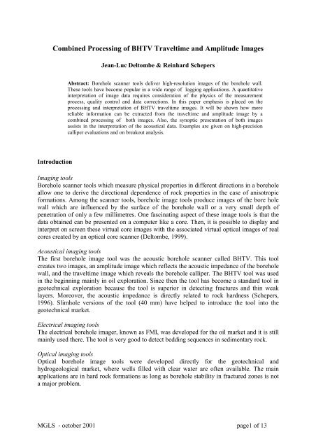
Combined Processing of BHTV Traveltime and Amplitude Images

Combined Processing of BHTV Traveltime and Amplitude Images 

Jean-Luc Deltombe & Reinhard Schepers 

Abstract: Borehole scanner tools deliver high-resolution images of the borehole wall. 

These tools have become popular in a wide range of logging applications. A quantitative 

interpretation of image data requires consideration of the physics of the measurement 

process, quality control and data corrections. In this paper emphasis is placed on the 

processing and interpretation of BHTV traveltime images. It will be shown how more 

reliable information can be extracted from the traveltime and amplitude image by a 

combined processing of both images. Also, the synoptic presentation of both images 

assists in the interpretation of the acoustical data. Examples are given on high-precision 

calliper evaluations and on breakout analysis. 

Introduction 

Imaging tools 

Borehole scanner tools which measure physical properties in different directions in a borehole 

allow one to derive the directional dependence of rock properties in the case of anisotropic 

formations. Among the scanner tools, borehole image tools produce images of the bore hole 

wall which are influenced by the surface of the borehole wall or a very small depth of 

penetration of only a few millimetres. One fascinating aspect of these image tools is that the 

data obtained can be presented on a computer like a core. Then, it is possible to display and 

interpret on screen these virtual core images with the associated virtual optical images of real 

cores created by an optical core scanner (Deltombe, 1999). 

Acoustical imaging tools 

The first borehole image tool was the acoustic borehole scanner called BHTV. This tool 

creates two images, an amplitude image which reflects the acoustic impedance of the borehole 

wall, and the traveltime image which reveals the borehole calliper. The BHTV tool was used 

in the beginning mainly in oil exploration. Since then the tool has become a standard tool in 

geotechnical exploration because the tool is superior in detecting fractures and thin weak 

layers. Moreover, the acoustic impedance is directly related to rock hardness (Schepers, 

1996). Slimhole versions of the tool (40 mm) have helped to introduce the tool into the 

geotechnical market. 

Electrical imaging tools 

The electrical borehole imager, known as FMI, was developed for the oil market and it is still 

mainly used there. The tool is very good to detect bedding sequences in sedimentary rock. 

Optical imaging tools 

Optical borehole image tools were developed directly for the geotechnical and 

hydrogeological market, where wells filled with clear water are often available. The main 

applications are in hard rock formations as long as borehole stability in fractured zones is not 

a major problem. 

MGLS - october 2001 page1 of 13

Scope of paper 

Acoustic image tools measure simultaneously two different images, i.e. an amplitude log 

which is directly related to geotechnical rock properties, and a traveltime log which allows 

one to derive a very precise borehole calliper. Even though finally two different physical 

parameter are recorded the two image logs are related to each other. We want to point out in 

this paper which information can be extracted by a combined processing of the two acoustic 

images and their synoptic interpretation. But our emphasis is placed on the processing and 

interpretation of traveltime image logs. 

Process of traveltime measurement 

Acoustical signal description 

W1 

W3 

Figure 1 

W2 

W4 

A typical signal send out and received by the acoustic transducer is schematically drawn in 

figure 1. The black line should be the signal which is recorded if there is no reflector. The first 

high amplitude wavelet is the transmitted signal followed by three coherent noise wavelets 

due to imperfect back damping or due to internal reflections inside the acoustic system. We 

assume that any incoherent electrical noise is always considerably smaller than any coherent 

acoustic noise. The level of such acoustic noise will limit a correct detection of traveltime in 

case of weak reflections from the borehole wall. 

Effect of noise 

The noise will, of course, depend on the acoustic components and the construction of the tool. 

But noise will also depend on the measurement window used during the recording of the 

image data. E.g. in figure 1 the window W1 is too close to the transmitted signal such that 

high amplitude values at the tail of the transmitted signal will result in a high noise level. A 

fixed long time window like W2 does not suffer from a potential wrong setting (W1) but it 

always includes the maximum coherent noise amplitude. The better approach is the individual 

optimal setting of the measurement window in accordance with the expected borehole calliper 

(W3 and W4). If the anticipated traveltimes fall into the gap between W3 and W4 and if 

reliable traveltime readings in areas of low reflection amplitudes are essential, an acoustic 

head with a different noise pattern can be used. 


Detection process 

Once a measurement window is defined the next influence on the traveltime measurement is 

given by the detection process of signals reflected at the borehole wall. An assumed weak 

reflection is overlayed as a red wavelet on the noise signal of figure 1. If a simple trigger level 

detection is used the reflected signal will not be detected in windows W1 and W2, and it will 

be very unlikely that it is detected in W3. The red wavelet will be properly detected if a 

maximum detection process is used. Modern BHTV tools record the full wave form of the 

reflected acoustic signal. As transmission of the full signal to the surface is not possible due to 

the limited data capacity of standard logging cables, fast on-line processing is therefore 

applied to realise a more sophisticated reflection signal detection. Such processing can use 

knowledge about the noise pattern and expected traveltimes to optimise the detection. Even 

the variation of the noise pattern with depth can be taken into account. Practically, such 

processing further reduces the length of the measurement window and moves the position of 

the window in an adaptive manner. In principle, this will allow one to detect the red wavelet 

in Windows W1, W2 and W3. But the situation depicted in figure 1 is fairly simple. The 

problem is more complex if the reflected signal is moving close to a noise signal. Finally 

constructive or destructive interference will change the signal form. If such a signal is 

detected at least the traveltime is close to the correct traveltime. On the other hand the 

amplitude is influenced considerably. 

Faulty detection 

Generally, we can state that in all cases where a wrong traveltime is detected, the amplitude is 

also wrong. On the other hand, the traveltime should be correct, if the amplitude is well above 

the noise level. As explained above the amplitude value can be wrong, even if the traveltime 

is correct. But this influence is only considerable at low amplitude values were relatively large 

amplitude variations can be assigned also to a number of other factors which are difficult to 

estimate properly. 

It is obvious that from the traveltime image an amplitude quality image can be derived which 

defines for each pixel, if the amplitude is reliable or if the amplitude is wrong. The procedure 

incorporates the definition of wrong traveltime reading so that in parallel a traveltime quality 

image is created. In addition, the amplitude image is used to further refine the traveltime 

quality image. But the traveltime quality image is still subjected to some ambiguity. Both 

quality images are used later during data processing and aid in a synoptic way in data 

interpretation procedures. 

Influence of directional resolution 

The performance and the usefulness of BHTV tools depend highly on their directional 

resolution. This resolution is defined by the width of the acoustic beam at the reflecting point, 

i.e. the borehole wall. 

Focused acoustical beam 

Figure 2 explains the principle features of a finely focused acoustic system. In the upper part 

of figure 2 the planar cross-section through the centre of a circular beam pattern is shown. 

Underneath the amplitude variation along the central axis of the beam is displayed. In the near 

field close to the transducer interference of acoustic energy results in rapid amplitude changes. 

From a certain distance on, the beam width and the amplitude stay more or less constant. The 

design goal for a good acoustic borehole system is to make the length (focal depth) of 

constant width and amplitude as long as possible. Optimum resolution and quantitative 

exploitable results are achieved if the reflection interface (borehole wall) is within the focal 


depth. The end distance of the focal depth depends on the frequency of the emitted signal and 

the aperture of the acoustic system. After the end of the focal depth the beam is spreading out 

at an angle of about 5 0 and the amplitude is decreasing rapidly. Slim hole BHTV tools with a 

typical acoustic frequency of 1 MHz allow one to realise beam width of 3mm and to expand 

the focal depth to 100mm. 

acoustic 

transducer 

Beam width 

amplitude 

along 

beam axis 

distance from transducer 

actual 

beam 

pattern 

Figure 2 

The lower part of figure 2 shows an actual beam pattern gained from laboratory experiments. 

The constant beam width spreads out from 25mm to 75mm. The amplitude along the beam is 

indicated by colour variations. 

Spike in travel time image 

1 

2 

3 

Figure 3 

Such highly focused acoustic systems are in a 

positive sense very sensitive to borehole 

conditions. We have referred already to wrong 

traveltime readings. Often it is argued that a 

good BHTV tool should not produce spiky 

traveltime images. This is definitely wrong. 

The physics of acoustic wave propagation 

require that under certain borehole conditions 

only very weak reflection can be expected and 

consequently no correct traveltime can be 

measured if the reflected amplitude is below 

the noise level. This means, the higher the 

dynamic range is of the acoustic system, the 

less spikes we get. But spikes cannot be 

avoided under all conditions. In figure 3, three 

situation are shown which will yield very weak 

or no reflections. 


Case 1 is an open fracture where most of the energy is refracted into the rock and only a very 

small part is reflected back to the transducer. 

Case 2 is a steeply dipping interface. The total energy is reflected downwards without 

reaching the transducer. 

Case 3 represent a thin zone of very low impedance which could be a very soft rock, a 

fracture or a mylonite zone. These zones are often accompanied by borehole washouts such 

that only some diffracting energy from the corner of the hard rock will reach the transducer. 

The better the resolution of a BHTV system, the more sensitive it is to not receive reflected 

energy in these cases described above. If a BHTV receives reflected signal in these cases the 

reflected energy can not come from the described structures. This means the real features are 

not correctly imaged. 

Comparison of good focused and bad focused system 

Figure 4 shall explain this with respect to a 

good focused and a bad focused system. 

1 

In case 1 the thin washed out zone is not 

detected by the unfocused system. In case 2 

the position of the edge and the transition 

2 

zone is not properly imaged by the 

unfocussed system. The same is true for 

case 3. In this last case we can expect the 

focused system to create one of those 

undesired spikes. But the spike tells us that 

3 the recorded amplitude is wrong and it 

gives a good estimate of the true position of 

the edge. As will be discussed later 

focused / unfocused beam processing of the traveltime data can 

remove the spikes from the data and can 

shape of bore hole wall 

recorded traveltime 

processed traveltime 

True edge position 

help to reconstruct the true borehole shape. 

The blue line illustrates this. 

Figure 5 compares the traveltime images 

(TT) and the amplitude images of a highresolution 

BHTV tool (HR) with those of a 

low-resolution BHTV tool (LR). All 

Figure 4 

structural features are considerably clearer 

in the HR amplitude image. E.g. a thin 

fracture at 12.8m is only visible in the HR image. The black dots in the HR-TT traveltime 

image indicate wrong traveltime readings. With respect to the LR-TT image one can rather 

speak of black areas, because faulty traveltimes spread out all along each detected fracture. 

With reference to the discussions above this can only be explained by a low dynamic range of 

the low-resolution system. The actually small calliper variations along the fractures are very 

well resolved by the HR-TT image. 


Figure 5 

Traveltime corrections 

Correction for faulty detection 

In most cases the detection of wrong traveltimes is a fairly simple and unique process. This is 

due to the fact that the surface of the borehole wall is highly 

oversampled with respect to calliper variation as the 

sampling interval is defined by the desired high resolution 

of the amplitude image. Oversampling of the traveltime 

image makes a lot of sense with respect to detection of true 

edge positions and the definition of the amplitude quality 

image which is important for the quantitative interpretation 

of the amplitude image. 

In figure 6a, a borehole cross-section of a more or less 

Figure 6a 

circular borehole is drawn. The dark circular line gives the 

true shape of the borehole. Some of these typical spikes 

occur in the cross-section display of the measured traveltime data if e.g. a fracture along the 

borehole creates low reflection amplitudes. As can be explained by figure 1 the spikes can go 

to the inside (case W1) or to the outside (case W2). The length of the spikes depends on the 

actual calliper and on the measurement window settings. No sophisticated processing is 

necessary to detect wrong traveltime data in this very common case 


The situation is more complicated if along a larger 

portion of the circumference there are many wrong 

readings and the true and wrong reading lie relatively 

close together such that a decision on wrong or right is 

difficult. The problem is illustrated by a cross-section 

display (figure 6b) as it is continuously monitored during 

field data acquisition. E.g. the traveltime readings in the 

upper right quadrant can be wrong but they may as well 

indicate a real breakout of the borehole wall. In this case 

a second run should be made where the traveltime quality 

image is refined by analysis of the amplitude image. 

Figure 6b 

Correction for decentralisation 

Detailed information about the borehole shape can be derived from the traveltime image. The 

BHTV tool does not really measure borehole calliper, rather it measures multiple distances 

from the tool to the borehole wall. Calliper is only defined with respect to the centre of a 

regular shaped borehole. 

Influence on travel time 

In figure 7 three different situation are schematically 

1 

presented. In case 1 the tool is decentralised in a circular 

borehole. The two green arrows indicate the two direction 

where the acoustic beam hits the borehole wall 

perpendicularly. Only at these two direction we get 

maximum reflection amplitudes and the addition of the two 

opposite traveltimes gives us the true borehole calliper. In 

2 

the direction of the two red arrows we measure a secant. 

The length of the secant depends on tool position. In case 3 

the tool is decentralised in an elliptical borehole. The 

borehole wall is hit perpendicularly in four directions. But it 

is quite obvious that the addition of the distance given by 

3 

the red arrows and distance in the opposite direction (green 

arrow) does not give a meaningful calliper value. Again, in 

case 2 the beam is perpendicular to the borehole wall in 

four directions. Calliper values can be calculated in all 

Figure 7 

directions, because the tool is in the centre of the borehole 

cross-section. In case of an irregular shaped borehole a 

“centre” is not uniquely defined. We will discuss later how the traveltime data can be used to 

define a centre in such a case. 


Figure 8 

Influence on amplitude 

As explained above the measured traveltime image depends on the position of the BHTV tool 

in the borehole. Figure 8 shows a typical result of a BHTV measurement. The traveltime is 

displayed in the left image track. We see a clear maximum (yellow) and minimum (blue) in 

the traveltime image. The difference between maximum and minimum is changing and also 

the direction of maximum and minimum. It is very likely in this case that the tool is not 

running along the centre of a more or less circular borehole (case 1 of figure 7). The amount 

of decentralisation and its direction is changing with depth. The traveltime image of figure 8 

does not tell us much about the borehole shape besides that we may assume a relatively 

smooth borehole wall. 

The information about decentralisation has its value with respect to the amplitude image. The 

influence of decentralisation (see figure 7) on the amplitude image in the middle track of 

figure 8 is visible as two broad shades (light brown) running parallel to the variation of the 

traveltime image. The narrow dark brown line in the amplitude image is due to tool 

construction. The shades and hence the influence of decentralisation can be removed to some 

extent from the amplitude image by a 2D high-pass filter. The result of the process is shown 

in the left track of figure 8. This image does not preserve the absolute variation of the 

amplitude values. Also, artefacts can be created in areas of rapid changes of the traveltime and 

amplitude image. Therefore, a crosscheck with both original images is recommended. 


Knowing the position of the tool we can add another information to the amplitude quality 

image. It marks the direction where the acoustic beam was perpendicular to the borehole wall. 

This information can be later used to derive a rock hardness log based on a reliable estimation 

of the reflection amplitude for each depth. 

Borehole shape calculation 

To come to the borehole shape, the first thing to do is to transfer the traveltime data into 

distance data relative to the centre of the borehole. Then, we can directly see the borehole 

shape if we display cross-sections of the distance data. Such an approach is not adequate if an 

overview over longer borehole intervals is required. Furthermore small details of borehole 

shape may not be visible as the display range of the traveltime data is governed by the amount 

of decentralisation. 

Figure 9 

Figure 9 shows some BHTV data with three different presentations of traveltime data. The 

first track on the left is a standard unrolled display of the traveltime image. According to the 

borehole cross-section in the third track the borehole is more or less circular. The track on the 

right shows a 3D displays where the distance image is use to create a perspective 3D view of 

borehole geometry. The amplitude data of track two is projected onto the 3D body. You may 

think: what a crooked hole the drillers have made. But you are wrong. The hole is perfectly 

straight. The borehole geometry appears to be so crooked because the distances are calculated 

relative to the actual tool position which is not constant. There are some small scale feature 

visible along the borehole. But it is difficult to decide if they are real or not. This example 


may point out how important it is to apply corrections to the distance image before a realistic 

3D display can be generated. 

We know the position of the tool relative to the borehole cross-section. This gives us the 

possibility to simulate in the computer the movement of the tool from its actual position to the 

centre of the borehole. The correction task is then to calculate the effect of such movement on 

each distance value. After the corrections are applied 

the distance image will look as if the tool has moved 

perfectly along the centre of the borehole. In the case of 

a regular borehole it is easy to define a centre of the 

borehole. The problem of the correction procedure is to 

adapt a practical approach for the calculation of the 

borehole centre. 

Figure 10 

In figure 10 a vertical projection of an inclined and 

irregular hole interval is indicated by two dark lines. 

Boreholes are drilled with a drill bit of a certain size and 

with drill strings with some rigidity and hence a 

minimum radius of curvature. Therefore, we define the 

centre of the borehole as the central axis of a pipe with 

the diameter of the drill bit which is fitted into the 

borehole with maximum curvature. One possibility to 

calculate the path of the virtual pipe has been described 

by Menger and Schepers, 1988. In all such calculation 

algorithm the information of the traveltime quality 

image should be implemented. A result of a pipe fitting 

process is presented in figure 10 by red lines. 

Traveltime interpretation and presentation 

High resolution calliper 

The result of a high resolution BHTV survey is shown in figure 11. 

The amplitude image on the left side exhibits many thin fractures. The uncorrected traveltime 

image in the middle indicates that along some fracture material is broken out, e.g. along the 

steeply dipping fracture at 42m. The amplitude image and the traveltime image were used to 

create the 3D display on the right side. Many spikes are visible along the borehole. As 

explained above the appearance of spikes under special borehole conditions (like open 

fractures) can be considered as a proof of the high resolution capability of the BHTV tool and 

the spikes identify pixels where no true amplitude is measured. Of course, in the final display 

of traveltime data we would like to present the true borehole shape without spikes. Also, this 

will be necessary to see small calliper variations. Using the traveltime quality image 

prediction and interpolation algorithm can be applied to calculate the distance value at those 

pixels where spikes occur. In many cases a 2D low-pass filter can help to remove the spikes 

and to reconstruct the borehole shape. If the preservation of edges is of importance (e.g. in 

breakout analysis) 2D medium filter (Castleman, 1979) –or more general 2D percentage filtershould 

be applied. 


Figure 11 

Presentation of very small (2 mm) bore hole caliper undulations induced by the drilling process 

Figure 12 


The results in figure 12 are a good example how much details of the borehole shape can be 

made visible after correction of the distance image for tool decentralisation and after removal 

of the spikes. The calliper image – or more correctly the distance image – is shown on the left 

side of figure 12. The amount and the good resolution of the calliper variations can be derived 

from the four tracks on the right which display individual calliper logs at four directions. As 

the scaling is from 40mm to 60mm the variations are in the range of only 2mm. The shape of 

the borehole is nicely revealed by the 3D display in figure 12. The scale is expanded such that 

the centre of the 3D display does not correspond to the centre of the borehole. Not the 

amplitude image but the calliper image is projected onto the borehole shape. The now clearly 

visible spiral along the borehole was created by the drilling process. 

Breakout analysis 

If the magnitude of maximum and 

minimum horizontal stress differ 

considerably from each other the borehole 

is deformed. These deformations lead to 

stress concentration and breakouts of the 

borehole wall occur in those intervals 

where the stress exceeds the strength of 

the rock (Barton, 1988). Typical for 

breakouts is that they develop on opposite 

sides of the borehole. The direction of the 

breakouts defines the direction of 

minimum horizontal stress. 

A very exciting way of breakout 

presentation can be realised with 3D 

presentation software which allows the 

user to move into all positions inside and 

outside the borehole and to look in all 

directions. Figure 13 displays one 

snapshot of such a presentation of a 

borehole section with breakouts. 

The 3D nicely reveals that breakouts are 

also visible on the amplitude image. This 

is due to the fact that the stress 

concentration has lead to deterioration of 

the rock. Acoustic measurement are very 

sensitive to detect defects in the rock. The 

blue colour (low amplitudes) in the 

amplitude image indicate these weak 

Figure 14 

zones which are wider than the breakouts 

itself. This means that some material is 

already partly destroyed but not yet broken out. Therefore, the amplitude image can be 

considered as an additional tool not only to see existing breakout but also to detect potential 

breakout areas. In the light of this new result the determination of the width of breakouts has 

to be carefully considered. 


Conclusion 

The high information content of BHTV images can be used in a wide range of logging 

applications where quantitative data evaluation is required. But prior to any quantitative 

interpretation it is essential to apply quality control, corrections and processing of the image 

data. Additional information is gained by a combined processing of the BHTV traveltime and 

amplitude images. Proper presentation and evaluation tools should assist the further 

interpretation process. New aspects of borehole breakout analysis could be revealed by 

adequate processing and presentation. 

References 

Barton, C.A., 1988. Development of In-situ Stress Measurement Techniques for Deep 

Drillholes, Dissertation, Stanford Rock & Borehole Project, 35, August 1988. 

Castleman, K.R., 1979. Digital Image Processing, Prentice Hall Inc., Englewood Cliffs, NJ. 

Deltombe, J.R., R. Schepers, and A. Toumani 1999. The practice of combined Core Image 

and Image Log interpretation for structural, lithological, sedimentological, and geotechnical 

applications. Proceedings of the International Symposium on Imaging Applications in 

Geology, University of Liège, Belgium. 

Menger, St. and R. Schepers, 1988. A Method to Derive High-Resolution Calliper Logs from 

Borehole Televiewer Traveltime Data, Proceedings of the 58 th Annual International SEG 

Meeting, p 554 – 556, Anaheim, CA. 

Schepers, R., 1996. Application of Borehole Logging to Geotechnical Exploration. 

Proceedings of the HANWHA Symposium, Seoul, Korea.

Combined Processing of BHTV Traveltime and Amplitude Images

Create successful ePaper yourself

Delete template?

Save as template?