Combining slash bundling with in-woods grinding operations
Combining slash bundling with in-woods grinding operations
Combining slash bundling with in-woods grinding operations

Create successful ePaper yourself
Turn your PDF publications into a flip-book with our unique Google optimized e-Paper software.
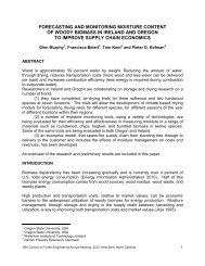
2009 Council on Forest Eng<strong>in</strong>eer<strong>in</strong>g (COFE) Conference Proceed<strong>in</strong>gs: “Environmentally Sound Forest Operations.”<br />
Lake Tahoe, June 15-18, 2009<br />
<strong>Comb<strong>in</strong><strong>in</strong>g</strong> <strong>slash</strong> <strong>bundl<strong>in</strong>g</strong> <strong>with</strong> <strong>in</strong>-<strong>woods</strong> gr<strong>in</strong>d<strong>in</strong>g <strong>operations</strong><br />
Hunter Harrill<br />
Graduate Research Assistant<br />
hh19@humboldt.edu<br />
Han-Sup Han<br />
Associate Professor of Forest Operations and Eng<strong>in</strong>eer<strong>in</strong>g<br />
Fei Pan<br />
Research Associate<br />
Department of Forestry and Wildland Resources<br />
College of Natural Resources & Sciences<br />
Humboldt State University<br />
Abstract<br />
Although extensive woody biomass resources are physically present, forest residues (i.e. logg<strong>in</strong>g<br />
<strong>slash</strong>) are under-utilized because collection and transportation costs are often greater than the<br />
market value of the materials and of the limited access to the site. This study quantified the<br />
operational cost and performance of a biomass harvest<strong>in</strong>g system utiliz<strong>in</strong>g a John Deere 1490D<br />
energy wood harvester, comb<strong>in</strong>ed <strong>with</strong> <strong>in</strong>-<strong>woods</strong> gr<strong>in</strong>d<strong>in</strong>g <strong>operations</strong>. The experiment took place<br />
at four recently harvested sites <strong>in</strong> northern California where logg<strong>in</strong>g <strong>slash</strong> was piled or scattered<br />
along the roadsides or across the clearcut units <strong>in</strong> various amounts and arrangements. Produced<br />
bundles were transported to a centralized process<strong>in</strong>g site where they were ground <strong>in</strong>to hog fuel<br />
and delivered to a local energy plant. Productivity for each phase of the operation ranged from 8<br />
to 42 bone dry tons (BDT)/productive mach<strong>in</strong>e hour (PMH), <strong>with</strong> a total production of 280.7<br />
BDT over 70.2 hours. The total system production cost was $60.98/BDT at 28.95% moisture<br />
content. Regression analysis <strong>in</strong>dicated that pile classification <strong>in</strong> terms of material size and<br />
arrangement had a significant impact on productivity of <strong>bundl<strong>in</strong>g</strong> (p
2004). Forest <strong>operations</strong> have the potential to supply 368 million dry tons of woody biomass<br />
annually (Perlack et al. 2005). The annual available biomass <strong>in</strong> California was estimated at 26.8<br />
million dry tons (Tiangco et al. 2005). Prescribed burn<strong>in</strong>g has long been the preferred method of<br />
dispos<strong>in</strong>g of forest biomass, but mechanical removal of biomass is becom<strong>in</strong>g more popular due<br />
to <strong>in</strong>creased restrictions on open field burn<strong>in</strong>g, or <strong>in</strong> areas like the wildland urban <strong>in</strong>terface<br />
(WUI) where burn<strong>in</strong>g is not an option.<br />
Forest residues are often not utilized because collection and transportation costs are greater than<br />
the market value of the materials (Withycombe 1982). Lack of research <strong>in</strong> this field has made<br />
harvest<strong>in</strong>g and transportation costs are notoriously difficult to estimate because there are critical<br />
gaps <strong>in</strong> the data and methods for predict<strong>in</strong>g costs (Rummer et al. 2008).<br />
New, more efficient harvest<strong>in</strong>g equipment like energy wood harvesters could reduce the<br />
associated process<strong>in</strong>g costs <strong>with</strong> their <strong>in</strong>creased productivity. These mach<strong>in</strong>es compact and<br />
bundle woody biomass <strong>in</strong>to log-shaped bundles, and could produce up to 40 half-ton bundles per<br />
hour <strong>with</strong> a production cost of $16 per dry ton (Rummer et al. 2004). Quantify<strong>in</strong>g costs and<br />
productivities of these new systems for biomass recovery from northern California will aid land<br />
managers <strong>in</strong> the plann<strong>in</strong>g and execution of cost-effective biomass supply for energy.<br />
The overall objective of this project was to determ<strong>in</strong>e the operational cost and performance of a<br />
biomass collection and densification system, called <strong>slash</strong> bundler, <strong>in</strong> comb<strong>in</strong>ation <strong>with</strong> a<br />
centralized gr<strong>in</strong>d<strong>in</strong>g operation. Important variables, such as haul<strong>in</strong>g distance and moisture<br />
contents, were itemized to understand their effects on productivity of collection and<br />
transportation. In particular, <strong>slash</strong> piles were characterized to evaluate the effect of <strong>slash</strong> type on<br />
productivity, based on arrangement and size of <strong>slash</strong> materials.<br />
Methodology<br />
Study site and system description<br />
The study was conducted <strong>in</strong> three clearcut harvest<strong>in</strong>g sites <strong>in</strong> northern California, rang<strong>in</strong>g from<br />
17 to 32 acres. The vegetation at each site varied but was generally dom<strong>in</strong>ated by second growth<br />
redwood (Sequoia sempervirens) and Douglas-fir (Pseudotsuga menziesii) <strong>with</strong> an average tree<br />
age of 60 years. The three sites had an average tree diameter at breast height (DBH) rang<strong>in</strong>g<br />
from 20-22 <strong>in</strong>ches, and ground slopes ranged from 0 to 30 percent. The stands were harvested<br />
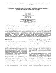
us<strong>in</strong>g a ground-based shovel logg<strong>in</strong>g system. There were many <strong>slash</strong> pile types <strong>in</strong> terms of size<br />
and arrangement present across these sites (Fig. 1). A forester work<strong>in</strong>g for the land owner<br />
suggested these sites were expected to yield anywhere from 50-75 tons/ac of <strong>slash</strong> from clearcut<br />
<strong>operations</strong> (Alcorn 2008).
Pile Class 1 = Mixed size material,<br />
loader piled<br />
Pile Class 2 = Large size material,<br />
processor piled<br />
Pile Class 3 = Mixed size material,<br />
side-cast piled<br />
Pile Class 4 = Mixed size material,<br />
processor piled<br />
Pile Class 5 = Small size material,<br />
loader piled<br />
Pile Class 6 = Mixed size material,<br />
side-cast<br />
Figure 1: Slash pile classification by arrangement and material size.<br />
A two week trial was conducted to collect and process woody residues after commercial timber<br />
harvest<strong>in</strong>g <strong>operations</strong>. The system collected material pre-piled at land<strong>in</strong>gs and along roadsides<br />
<strong>with</strong> a <strong>slash</strong> bundler (John Deere 1490D). The bundler compacted and wrapped <strong>slash</strong> <strong>in</strong>to 10ft<br />
long bundles <strong>with</strong> an average diameter of 27 <strong>in</strong>ches. Bundles were then loaded <strong>in</strong>to 40 cubic yard<br />
conta<strong>in</strong>ers along the roadside <strong>with</strong> a loader (Hitachi EX 200-3). The bundles were delivered to a<br />
nearby central gr<strong>in</strong>d<strong>in</strong>g location (< 3 miles; Fig. 3) by hook-lift trucks. A gr<strong>in</strong>der (Peterson<br />
Pacific 7400) was set up at the centralized gr<strong>in</strong>d<strong>in</strong>g site and ground all the bundles <strong>in</strong>to hog fuel.<br />
Hog fuel was then belt fed <strong>in</strong>to 120 cubic yard chip vans and transported to a local power plant.
Figure 2: John Deere 1490D energy wood harvester which produces the bundles, and hook-lift<br />
truck used to haul bundles.<br />
Dirt road<br />
0.92<br />
miles<br />
Unit A<br />
2⁰ Gravel road<br />
0.68<br />
miles<br />
Unit B<br />
1⁰ Gravel road<br />
1.64<br />
miles<br />
Unit C<br />
Centralized<br />
gr<strong>in</strong>d<strong>in</strong>g<br />
site<br />
Figure 3: Operation layout map <strong>with</strong> correspond<strong>in</strong>g road segments.<br />
Data collection and analysis<br />
Hourly mach<strong>in</strong>e costs (Table 2) measured <strong>in</strong> dollars per scheduled mach<strong>in</strong>e hour (SMH) were<br />
calculated us<strong>in</strong>g standard mach<strong>in</strong>e rate calculation method (Miyata 1980). For each mach<strong>in</strong>e <strong>in</strong><br />
the system purchase price, <strong>in</strong>surance and tax rates, repair costs, fuel consumption, and labor costs<br />
were obta<strong>in</strong>ed from the contractor, diesel fuel price receipts were averaged throughout length of<br />
the operation ($4.60/gal). All mach<strong>in</strong>ery were assumed to work 1800 SMH annually and have an<br />
economic life of ten years except for the gr<strong>in</strong>der which was 5 year economic life due to<br />
associated wear, and the bundler which was assumed to work 2100 SMH as suggested by John<br />
Deere Company.
Time study data was collected to calculate hourly production (bone dry ton (BDT)/productive<br />
mach<strong>in</strong>e hour (PMH)) us<strong>in</strong>g standard time study techniques for each element <strong>in</strong> a mach<strong>in</strong>es<br />
operation cycle by stop watch (Olsen et al. 1998). A <strong>bundl<strong>in</strong>g</strong> cycle <strong>in</strong>cludes travel<strong>in</strong>g to the<br />
<strong>slash</strong> pile, followed by multiple grapples and sw<strong>in</strong>gs of <strong>slash</strong> to the <strong>in</strong>-feed table, and ended<br />
when the bundle produced was cut free from the mach<strong>in</strong>e. A load<strong>in</strong>g cycle started from travel<strong>in</strong>g<br />
to a bundle, followed by sw<strong>in</strong>g<strong>in</strong>g empty to the bundle, grappl<strong>in</strong>g the bundle, sw<strong>in</strong>g<strong>in</strong>g loaded<br />
back to the conta<strong>in</strong>er, and ended by compact<strong>in</strong>g bundle <strong>in</strong>to the conta<strong>in</strong>er. A hook-lift truck<strong>in</strong>g<br />
cycle <strong>in</strong>cludes travel<strong>in</strong>g empty to the harvest unit, position<strong>in</strong>g the truck for load<strong>in</strong>g, load<strong>in</strong>g a<br />
conta<strong>in</strong>er filled <strong>with</strong> bundles, travel<strong>in</strong>g loaded to the centralized gr<strong>in</strong>d<strong>in</strong>g site, and<br />
unload<strong>in</strong>g/dump<strong>in</strong>g the bundles. Three types of delay time, <strong>in</strong>clud<strong>in</strong>g operational delays,<br />
mechanical delays and personal delays, were recorded.<br />
Regression models for delay-free cycle time were developed us<strong>in</strong>g the pre-identified <strong>in</strong>dependent<br />
variables associated <strong>with</strong> each cycle. The collected time study data were screened for normality<br />
and outliers us<strong>in</strong>g histograms and residual plots, and were used to develop predictive equations<br />
by runn<strong>in</strong>g multiple regressions us<strong>in</strong>g ord<strong>in</strong>ary least squares estimators, performed <strong>in</strong> R 2.4.1<br />
statistical software program (R 2006). The f<strong>in</strong>al predictive models only <strong>in</strong>clude variables that<br />
were statistically significant (p-value
undl<strong>in</strong>g, load<strong>in</strong>g and haul<strong>in</strong>g, and gr<strong>in</strong>d<strong>in</strong>g stages of operation respectively. Regional delivered<br />
hog fuel prices dur<strong>in</strong>g the time of study was surveyed at $50 a bone dry ton (BDT).<br />
Results & Discussion<br />
Cycle time regression equations<br />
Regression equations developed from the time study data <strong>with</strong> significant variables (p < 0.05, α<br />
= 0.05) were summarized <strong>in</strong> Table 3. Both models for the bundler and the hook-lift truck had<br />
high r-squared values, <strong>in</strong>dicat<strong>in</strong>g that they might be effective <strong>in</strong> estimat<strong>in</strong>g the productivity for<br />
load<strong>in</strong>g and haul<strong>in</strong>g.<br />
Bundl<strong>in</strong>g cycle time was affected ma<strong>in</strong>ly by different handl<strong>in</strong>g and arrang<strong>in</strong>g activities such as,<br />
the number of grapples to pick up <strong>slash</strong>, or the number of <strong>in</strong>-feeds to place the <strong>slash</strong> on the <strong>in</strong>feed<br />
table for <strong>bundl<strong>in</strong>g</strong>. The grappl<strong>in</strong>g element consumed the greatest amount of time dur<strong>in</strong>g an<br />
average <strong>bundl<strong>in</strong>g</strong> cycle (0.85 m<strong>in</strong>utes, 44.5%), while the travel<strong>in</strong>g element was responsible for<br />
the smallest portion of cycle time (0.09 m<strong>in</strong>utes, 4.8%; Figure 4). This was most likely due to the<br />
fact that the mach<strong>in</strong>e could rema<strong>in</strong> stationary because of the amount of <strong>slash</strong> available <strong>with</strong><strong>in</strong><br />
reach, and spent the greatest of time grappl<strong>in</strong>g <strong>in</strong> order to properly align <strong>slash</strong> for efficient <strong>in</strong>feed<strong>in</strong>g.<br />
The regression equation also <strong>in</strong>dicated that the number of sw<strong>in</strong>g cycles for which the<br />
bundler picks up <strong>slash</strong> and places it on the <strong>in</strong>-feed table had a significant effect on cycle time.<br />
When consider<strong>in</strong>g the effect of pile classification on estimated <strong>bundl<strong>in</strong>g</strong> cycle time, pile class 1,<br />
pile class 2, and pile class 6 were the only pile classes found to be statistically significant (pvalue<br />
Grappl<strong>in</strong>g the bundles and compact<strong>in</strong>g them <strong>in</strong>to the b<strong>in</strong> proves to significantly affect the load<strong>in</strong>g<br />
cycle time. Loaded sw<strong>in</strong>g degrees <strong>in</strong> which the mach<strong>in</strong>e had to rotate to place a bundle <strong>in</strong> the b<strong>in</strong><br />
was also found to be significant, along <strong>with</strong> the travel distance necessary to reach a bundle. The<br />
regression analysis suggests that decreas<strong>in</strong>g the travel distance and m<strong>in</strong>imiz<strong>in</strong>g sw<strong>in</strong>g degrees<br />
would greatly reduce the predicted cycle time.<br />
The transportation distance along various road types positively affected the haul<strong>in</strong>g cycle time.<br />
Only loaded haul<strong>in</strong>g distances were used to develop the truck<strong>in</strong>g regression equation because the<br />
same routes were used to and from harvest units. The position<strong>in</strong>g distance for a hook-lift truck to<br />
position himself to be loaded was also found to have a significant effect on cycle time because<br />
this was done while driv<strong>in</strong>g <strong>in</strong> reverse, and had to be done carefully to properly align himself for<br />
load<strong>in</strong>g by the Hitachi loader.<br />
Table 3: Delay-free average cycle time equations for <strong>bundl<strong>in</strong>g</strong>, load<strong>in</strong>g, and haul<strong>in</strong>g activities.<br />
Mach<strong>in</strong>e Average cycle time estimator (centim<strong>in</strong>utes) Variable range Mean r² n P-value F-stat Standard error ¹<br />
Bundler = 3.87 0.81 300 0.17<br />
+ 0.03 (travel distance <strong>in</strong> feet) 0-280 5.56 < 0.0001 72.27<br />
+ 0.54 (number of grapples) 1-22 7.61 < 0.0001 303.35<br />
+ 0.41 (number of <strong>in</strong>feeds) 1-11 4.40 < 0.0001 111.45<br />
- 0.20 (number of sw<strong>in</strong>g cycles) 1-8 4.52 < 0.0001 14.82<br />
- 0.08 (pile class 1) 0.002<br />
+ 0.13 (pile class 2) < 0.0001<br />
- 0.11 (pile class 3) 0.092<br />
- 0.03 (pile class 4) 0.305<br />
- 0.03 (pile class 5) 0.210<br />
+ 0.13 (pile class 6) 0.038<br />
Loader = 3.88 0.54 465 0.20<br />
+ 0.45 (number of compactions) 1-5 1.23 < 0.0001 216.42<br />
+ 0.06 (travel distance <strong>in</strong> feet) 0-220 1.51 < 0.0001 164.41<br />
+ 0.42 (number of grapples) 1-3 1.08 < 0.0001 66.76<br />
+ 0.22 (loaded sw<strong>in</strong>g degrees) 90-270 126.81 < 0.0001 72.08<br />
+ 0.09 (% slope) 5-10 6.58 0.003 8.99<br />
Hook-lift truck = 987.40 0.84 30 344.97<br />
+ 0.22 (loaded primary gravel road distance <strong>in</strong> feet) 2189-8635 7436.27 < 0.0001 30.16<br />
+ 0.22 (loaded dirt road distance <strong>in</strong> feet) 200-4846 2423.97 < 0.0001 38.56<br />
+ 1.44 (position for load<strong>in</strong>g distance <strong>in</strong> feet) 10-600 261.33 0.011 7.47<br />
pile class 1 = mixed size material, loader piled<br />
pile class 2 = large size material, processor piled<br />
pile class 3 = mixed size material, side-cast piled<br />
pile class 4 = mixed size material, processor piled<br />
pile class 5 = small size material, loader piled<br />
pile class 6 = mixed size material, side-cast<br />
Production rates<br />
The hourly production of each mach<strong>in</strong>e was determ<strong>in</strong>ed by divid<strong>in</strong>g the average weight of<br />
bundles or b<strong>in</strong>s (tons) by the predicted cycle time (m<strong>in</strong>utes). Average predicted delay-free cycle<br />
time for the bundler to make one ten foot long bundle was 1.74 m<strong>in</strong>utes, mean<strong>in</strong>g the mach<strong>in</strong>e<br />
produced about 34 bundles per productive mach<strong>in</strong>e hour. With the bundles hav<strong>in</strong>g an average<br />
moisture content of 22.55%, and an average length and diameter of 10.1ft and 27.6 <strong>in</strong>ches<br />
respectively, the bundler productivity was determ<strong>in</strong>ed at 8.03 BDT/PMH (Table 4).
Us<strong>in</strong>g the predicted model for the bundler and hold<strong>in</strong>g all other variables constant pile class 2<br />
and pile class 6 resulted <strong>in</strong> the longest predicted cycle time of 2.04 m<strong>in</strong>utes (Table 4; Table 5).<br />
Pile class 3 yielded the smallest predicted cycle time of 1.60 m<strong>in</strong>utes. The difference <strong>in</strong> predicted<br />
cycle time between piles is l<strong>in</strong>ked <strong>with</strong> grappl<strong>in</strong>g, which consumes the largest portion of a total<br />
<strong>bundl<strong>in</strong>g</strong> cycle. Processor piled materials are generally aligned parallel which is preferable for<br />
the bundler because of the reduced need for grappl<strong>in</strong>g, but larger size materials are harder to<br />
grapple and don’t bundle as well result<strong>in</strong>g <strong>in</strong> poor bundle <strong>in</strong>tegrity. When loaders pile material<br />
they tend to rake the <strong>slash</strong> <strong>in</strong>to heap<strong>in</strong>g piles <strong>with</strong> lots of air space and poor material alignment,<br />
which is negligible consider<strong>in</strong>g the mach<strong>in</strong>e’s compact<strong>in</strong>g force, especially when smaller size<br />
materials are bundled.<br />
Table 4: Predicted delay-free average cycle time and production rate.<br />
Bundler Loader Hook-lift truck<br />
Cycle time Prod. Rate Cycle time Prod. Rate Cycle time Prod. Rate<br />
(m<strong>in</strong>) (BDT¹/PMH²) (m<strong>in</strong>) (BDT/PMH) (m<strong>in</strong>) (BDT/PMH)<br />
Unit A 1.72 8.23 0.46 41.22 34.28 11.49<br />
Unit B 1.93 7.30 0.44 42.77 42.83 9.20<br />
Unit C 1.61 8.77 0.43 43.33 22.37 17.61<br />
Overall 1.76 8.04 0.44 42.32 35.43 11.12<br />
¹BDT: bone dry ton<br />
²PMH: productive mach<strong>in</strong>e hour<br />
Table 5: Bundl<strong>in</strong>g productivity predicted us<strong>in</strong>g regression equations based on <strong>slash</strong> Pile<br />
Classifications.<br />
Pile Class¹ # Bundles Avg. time (m<strong>in</strong>/bundle) Tons/PMH # Bundles/PMH<br />
1 70 1.66 8.7 36<br />
2 31 2.04 7.1 29<br />
3 5 1.60 9.0 37<br />
4 148 1.75 8.2 34<br />
5 40 1.73 8.4 35<br />
6 6 2.04 7.1 29<br />
¹ Refer to Figure 1 or Table 3<br />
Average predicted delay-free cycle time for the loader to pick up a bundle, and place it <strong>in</strong> a b<strong>in</strong><br />
took 0.44 m<strong>in</strong>utes or 26 seconds (Table 4). It took an average of 21 cycles or 9 m<strong>in</strong>utes to fill an<br />
entire b<strong>in</strong> <strong>with</strong> bundles which had an average weight of 6.6 BDT, mean<strong>in</strong>g the loader could<br />
produce and astound<strong>in</strong>g 42.32 BDT/PMH. The compact<strong>in</strong>g element <strong>in</strong> a load<strong>in</strong>g cycle was the<br />
most time consum<strong>in</strong>g part of the load<strong>in</strong>g process due to the time used to carefully stack and<br />
maximize the number of bundles <strong>in</strong>side the b<strong>in</strong>. Travel<strong>in</strong>g took the least amount of time (0.01<br />
m<strong>in</strong>utes, 3.1%) because the bundles were properly roadside decked m<strong>in</strong>imiz<strong>in</strong>g the operators<br />
need of travel.
The delay-free truck<strong>in</strong>g cycle took on average 35 m<strong>in</strong>utes, <strong>with</strong> a production rate of 11.1<br />
BDT/PMH (Table 4). Load<strong>in</strong>g the b<strong>in</strong> consumed the greatest percentage of the cycle time<br />
(37.2%, 11 m<strong>in</strong>utes) and was longer on average than unload<strong>in</strong>g the b<strong>in</strong> because a truck had to<br />
wait to be loaded at the harvest site by the Hitachi loader. Whereas the unload<strong>in</strong>g of a b<strong>in</strong> took<br />
less time (2 m<strong>in</strong>utes), the driver would tilt the b<strong>in</strong> back and then pull forward to empty the<br />
contents like a dump truck. If possible b<strong>in</strong>s should be pre-loaded on site and then picked up by<br />
the hook-lift truck. Pre-load<strong>in</strong>g of b<strong>in</strong>s could reduce total cycle time by up to 8 m<strong>in</strong>utes,<br />
<strong>in</strong>creas<strong>in</strong>g the haul<strong>in</strong>g production to nearly 14 BDT/PMH.<br />
The average observed time for the gr<strong>in</strong>der to belt feed a chip van was 21 m<strong>in</strong>utes, which carried<br />
on average 20.8 BDT/load. Gr<strong>in</strong>d<strong>in</strong>g activities produced a total of 280.7 BDT over a total of 8<br />
hours or 33.14 BDT/PMH.<br />
Table 6: Road type, one-way distance, and average ⁰ travel speed.<br />
⁰<br />
Harvest site Spur road Dirt road 2 Gravel road 1 Gravel road Total<br />
--------------------------------(miles)-------------------------------<br />
Unit A 0.53 0.29 0.68 1.64 2.61<br />
Unit B 0.25 0.92 0 1.58 2.5<br />
Unit C 0.25 0.04 0 0.41 0.45<br />
Avg. Speed (miles/hr) 5.3 8.0 18.0 22.7<br />
⁰<br />
Average ⁰ speed = distance/observed time traveled<br />
1 Gravel road = double lane rocked road<br />
2 Gravel road = s<strong>in</strong>gle lane rocked road<br />
Dirt road = s<strong>in</strong>gle lane seasonal dirt road constructed <strong>with</strong> native soils<br />
Spur road = unimproved temporary dirt spur <strong>with</strong><strong>in</strong> harvest unit<br />
Production costs<br />
The production costs ($/ton) <strong>in</strong>clud<strong>in</strong>g <strong>bundl<strong>in</strong>g</strong>, load<strong>in</strong>g, haul<strong>in</strong>g, gr<strong>in</strong>d<strong>in</strong>g and support<strong>in</strong>g<br />
activities was $44.94/GT or $60.98/BDT (Table 7). Wet-based moisture content of the <strong>slash</strong><br />
dur<strong>in</strong>g <strong>bundl<strong>in</strong>g</strong> was 22.55% which <strong>in</strong>creased to 24.27% dur<strong>in</strong>g load<strong>in</strong>g and haul<strong>in</strong>g stages, and<br />
f<strong>in</strong>ally <strong>in</strong>creased to 28.95% dur<strong>in</strong>g gr<strong>in</strong>d<strong>in</strong>g. The <strong>in</strong>crease <strong>in</strong> percent moisture content was most<br />
likely a result of heavy fog, and the two days of ra<strong>in</strong> that occurred dur<strong>in</strong>g gr<strong>in</strong>d<strong>in</strong>g.<br />
The average cost of gr<strong>in</strong>d<strong>in</strong>g $17.97/BDT was the most costly process of the system,<br />
represent<strong>in</strong>g nearly one third of the total production cost. The high cost of gr<strong>in</strong>d<strong>in</strong>g<br />
($595.71/PMH) reflects the cost of runn<strong>in</strong>g the gr<strong>in</strong>der, front-end loader, and Hitachi loader<br />
simultaneously, which is necessary <strong>in</strong> order to achieve the high level of production (33.14<br />
BDT/PMH).<br />
Bundl<strong>in</strong>g production costs (16.20/BDT) was the second highest component of system cost, due<br />
to the high hourly cost $133/PMH and the low production rate of 8.04BDT/PMH. Load<strong>in</strong>g<br />
bundles <strong>in</strong>to b<strong>in</strong>s proved to be the most cost effective stage of the harvest<strong>in</strong>g system <strong>with</strong> a<br />
production cost of $2.99/BDT, primarily due to the mach<strong>in</strong>es high rate of production (42.32<br />
BDT/PMH), the highest <strong>in</strong> the system. The densification of <strong>slash</strong> <strong>in</strong>to bundles makes the material
easier to handle, and <strong>in</strong>creases the average weight per cycle, thus improv<strong>in</strong>g productivity of<br />
load<strong>in</strong>g and haul<strong>in</strong>g stages while reduc<strong>in</strong>g their production costs. However, the bottleneck <strong>in</strong> this<br />
system appears to be the <strong>bundl<strong>in</strong>g</strong> stage, <strong>with</strong> a low production rate production compared to the<br />
next stage of load<strong>in</strong>g. Decoupl<strong>in</strong>g the <strong>bundl<strong>in</strong>g</strong> stage may reduce the potential system bottleneck<br />
by creat<strong>in</strong>g a buffer of bundles to be loaded and hauled, thus maximiz<strong>in</strong>g a loaders utilization<br />
rate.<br />
Support costs are often an overlooked component of forest <strong>operations</strong>. Fuel trucks are needed to<br />
deliver and fuel to exist<strong>in</strong>g mach<strong>in</strong>ery, water trucks are required for dust abatement purposes,<br />
and service trucks have the tools and parts necessary for daily ma<strong>in</strong>tenance and repairs. The<br />
support cost ($14.48/BDT) <strong>in</strong> this system is the third largest component of total system cost, this<br />
<strong>in</strong>cludes the cost of own<strong>in</strong>g all of the support vehicles and their assumed use of 30 m<strong>in</strong>utes daily<br />
divided by the total tons produced dur<strong>in</strong>g the operation 280.7 BDT. System supports costs may<br />
be greatly reduced if the operation were to be full scale, by <strong>in</strong>creas<strong>in</strong>g the total tons produced.<br />
Table 7: Estimated system production and cost.<br />
Bundl<strong>in</strong>g Load<strong>in</strong>g Haul<strong>in</strong>g Gr<strong>in</strong>d<strong>in</strong>g Support Total ¹<br />
Hourly Cost ($/PMH) ² $ 133.19 $126.60 $103.84 $595.71 $57.88 $1,017.22<br />
Hourly Production (GT/PMH) ⁴<br />
$ 10.62 55.88 14.68 46.65 N/A<br />
Cost ($/GT) ³ $ 12.55 $2.27 $7.07 $12.77 $10.29 $44.94<br />
Cost ($/BDT)<br />
$ 16.20 $2.99 $9.34 $17.97 $14.48 $60.98<br />
Moisture content for <strong>bundl<strong>in</strong>g</strong> was 22.55%, 24.27% <strong>in</strong> load<strong>in</strong>g and haul<strong>in</strong>g, and 28.95% dur<strong>in</strong>g gr<strong>in</strong>d<strong>in</strong>g.<br />
¹ Total system cost does not <strong>in</strong>clude move <strong>in</strong> costs, transportation to market, or profit allowance.<br />
² ⁴ PMH: productive mach<strong>in</strong>e hour<br />
³ GT: green ton<br />
BDT: bone dry ton<br />
Haul<strong>in</strong>g the bundles to the centralized gr<strong>in</strong>d<strong>in</strong>g site cost $9.34/BDT the second lowest<br />
component of system cost. Haul<strong>in</strong>g costs represented approximately 15% of the total production<br />
cost, but proved to be highly variable depend<strong>in</strong>g on road conditions. Sensitivity analysis<br />
<strong>in</strong>dicates m<strong>in</strong>imiz<strong>in</strong>g road types such as s<strong>in</strong>gle lane dirt roads which have travel<strong>in</strong>g speeds of less<br />
than 10 mph greatly improves truck<strong>in</strong>g productivity and reduces production costs (Fig. 5).<br />
Hold<strong>in</strong>g all other variables of system cost constant, every mile <strong>in</strong>crease of dirt road haul<strong>in</strong>g<br />
distance will cause a $3.07/BDT <strong>in</strong>crease <strong>in</strong> total system cost. Due to the variability <strong>in</strong><br />
transportation costs and the high costs associated <strong>with</strong> haul<strong>in</strong>g on forest roads, it suggested that a<br />
harvest site should be located no more than 5 miles away from the centralized gr<strong>in</strong>d<strong>in</strong>g site.
System cost<br />
($/BDT)<br />
78.00<br />
76.00<br />
74.00<br />
72.00<br />
70.00<br />
68.00<br />
66.00<br />
64.00<br />
62.00<br />
60.00<br />
1 1.5 2 2.5 3 3.5 4<br />
Dirt road miles<br />
1⁰ gravel road<br />
miles<br />
1<br />
2<br />
3<br />
Figure 5: Sensitivity analysis of system production cost on various transportation distances.<br />
One factor that had an effect on the overall system cost was diesel fuel prices which were at a<br />
national peak dur<strong>in</strong>g the study <strong>in</strong> the summer of 2008. Diesel fuel price assumed for the<br />
operation was $4.60/gal. Six months later fuel prices <strong>in</strong> the region dropped to $2.50/gal. Hold<strong>in</strong>g<br />
all other variables of system cost constant, every dollar reduction of fuel price represents around<br />
a $3.52/BDT reduction <strong>in</strong> overall system cost (Fig. 6).<br />
Production Cost<br />
($/BDT)<br />
64<br />
62<br />
60<br />
58<br />
56<br />
54<br />
52<br />
50<br />
2.00 2.25 2.50 2.75 3.00 3.25 3.50 3.75 4.00 4.25 4.50 4.75 5.00<br />
Diesel Fuel Price<br />
($/gal)<br />
Figure 6: Sensitivity analysis on system production cost <strong>with</strong> various fuel market<br />
prices.
Conclusion<br />
This study evaluated harvest<strong>in</strong>g productivity and cost of a woody biomass recovery system us<strong>in</strong>g<br />
a <strong>slash</strong> bundler. Productivity for different mach<strong>in</strong>es varied from 8 to 42 BDT/PMH, <strong>with</strong> a total<br />
production of 280.7 BDT over 70.2 hours. Production cost ranged from $2.99 to $17.97/BDT for<br />
different system components, <strong>with</strong> a total system production cost of $60.98/BDT at 28.95%<br />
moisture content.<br />
The bundler tested on ground based clearcut sites performed well produc<strong>in</strong>g 29-37 10ft bundles<br />
per productive mach<strong>in</strong>e hour. Slash pile arrangement and material size were found to have a<br />
significant effect on productivity of <strong>bundl<strong>in</strong>g</strong>. Pile class 3 (typical size material, side-cast piled)<br />
was found to be the most effective pile type when consider<strong>in</strong>g <strong>bundl<strong>in</strong>g</strong> productivity, yield<strong>in</strong>g<br />
the smallest predicted cycle time (1.60 m<strong>in</strong>utes).<br />
Load<strong>in</strong>g <strong>slash</strong> <strong>in</strong>to b<strong>in</strong>s was efficient and had a low cost of $2.99/BDT. Load<strong>in</strong>g costs could be<br />
<strong>in</strong>flated if the bundles were not located <strong>with</strong><strong>in</strong> one sw<strong>in</strong>g of the road edge because of <strong>in</strong>creased<br />
travel distance. The hook-lift truck effectively negotiated adverse forest roads and allowed the<br />
removal of <strong>slash</strong> from traditionally difficult- to-access sites, <strong>with</strong>out burn<strong>in</strong>g <strong>slash</strong>. Harvest sites<br />
ideally should be located <strong>with</strong><strong>in</strong> close proximity to a centralized gr<strong>in</strong>d<strong>in</strong>g site (< 5 miles).<br />
Due to the complexity of variables and their effects on overall system cost and productivity, it is<br />
apparent that <strong>operations</strong> like the one observed <strong>in</strong> this study require careful plann<strong>in</strong>g and strategic<br />
logistical arrangements. System cost can drastically change <strong>with</strong> <strong>in</strong>creased haul<strong>in</strong>g mileage on<br />
s<strong>in</strong>gle lane dirt roads, due to slow travel<strong>in</strong>g speeds (8 mph). The total system cost will <strong>in</strong>crease<br />
$3.07/BDT for every one mile <strong>in</strong>crease <strong>in</strong> dirt road haul<strong>in</strong>g distance. The cost of the fuel price<br />
was found to have a tremendous effect on total system cost, every $1/gal fuel price <strong>in</strong>crease<br />
would result <strong>in</strong> a system cost <strong>in</strong>crease of $3.52/BDT.<br />
Forest biomass was removed successfully from previously harvested timber sites <strong>with</strong> poor<br />
access issues, but the overall system production cost was still high. The high system cost is<br />
primarily due to the poor system balance and the low level of production associated <strong>with</strong> be<strong>in</strong>g<br />
an experimental rather than full scale operation. Appropriate pair<strong>in</strong>gs of mach<strong>in</strong>es may further<br />
reduce system bottlenecks and greatly improve the system productivity which may further reduce<br />
system cost.
Literature Cited<br />
Alcorn, M.W.2008. Personal communication. Forester. Green Diamond Resource Company.<br />
Korbel, CA.<br />
Ba<strong>in</strong>, R.L.; Amos, W.A.; Down<strong>in</strong>g, M.; Perlack, R.L. 2003. Biopower technical assessment:<br />
state of the <strong>in</strong>dustry and the technology. NREL Rep. TP-510-33123. Golden, CO:<br />
National Renewable Energy Laboratory. 277 p.<br />
Beckert, E.; Jakle, A. 2008. Renewable energy data book. U.S. Department of Energy, Energy<br />
Efficiency and Renewable Energy. 131p.<br />
Evans, A.M. 2008. Synthesis of woody biomass removal case studies. U.S. Department of<br />
Agriculture, Forest Service. Forest Guild September. 39p.<br />
Han, H.-S.; H.W. Lee; L.R. Johnson. 2004. Economic feasibility of an <strong>in</strong>tegrated harvest<strong>in</strong>g<br />
system for small-diameter trees <strong>in</strong> southwest Idaho. Forest Products Journal. 54: 21-<br />
27.<br />
Han, H.-S. 2008. Economic evaluation of roll-off conta<strong>in</strong>ers used to collect forest biomass<br />
result<strong>in</strong>g from shaded fuelbreak treatments. Submitted to Six Rivers National Forest.<br />
28p.<br />
Miyata, E.S. 1980. Determ<strong>in</strong><strong>in</strong>g fixed and operat<strong>in</strong>g costs of logg<strong>in</strong>g equipment. General<br />
Technical Report NC-55. USDA Forest Service, North Central Forest Experiment<br />
Station. St. Paul, M<strong>in</strong>nesota. 16p.<br />
Nicholls, D.L.; R.A. Monserud; D.P. Dykstra. 2008. A synthesis of biomass utilization for<br />
bioenergy production <strong>in</strong> the Western United States. Gen. Tech. Rep. PNW-GTR-753.<br />
Portland, OR: U.S. Department of Agriculture, Forest Service, Pacific Northwest<br />
Research Station. 48p.<br />
Olsen, E.D.; M.N. Hossa<strong>in</strong>; M.E. Miller. 1998. Statistical comparison of methods used <strong>in</strong><br />
harvest<strong>in</strong>g work studies. Forest Research Laboratory, Oregon State University,<br />
Research contribution. 23: 41p.<br />
Perlack, R.; L. Wright; A. Turhollow; R. Graham. 2005. Biomass as feedstock for a bioenergy<br />
and bioproducts <strong>in</strong>dustry: the technical feasibility of a billion-ton annual supply.<br />
Prepared for the U.S. Department of Energy, Oak Ridge National Laboratory,<br />
ORNL/TM-2005/66, 65p.<br />
Rawl<strong>in</strong>gs, C.; B. Rummer; C. Seeley; C. Thomas; D. Morrison; H.-S. Han; L. Cheff, D. Atk<strong>in</strong>s;<br />
D. Graham; K.W<strong>in</strong>dell. 2004. A study of how to decrease the costs of collect<strong>in</strong>g,<br />
process<strong>in</strong>g and transport<strong>in</strong>g <strong>slash</strong>. Montana Community Development Corporation,<br />
Missoula, Montana, 21p.
Rummer, B. 2008. Assess<strong>in</strong>g the cost of fuel reduction treatments: a critical review. Forest<br />
Policy and Economics. 10: 355-362.<br />
Rummer, B.; D. Len; O. O’Brien. 2004. Forest residues <strong>bundl<strong>in</strong>g</strong> project: new technology for<br />
residue removal. USDA Forest Serv., Forest Operations Research unit, Southern<br />
Research Sta. Auburn, AL. 17p.<br />
Tiangco, V., G. Simmons, R. Kukulka, S. Matthews. 2005. Biomass resource assessment <strong>in</strong><br />
California. Prepared for the California Energy Commission, Public Interest Energy<br />
Research Program, CEC-500-2005-006-D, 54p.<br />
Withycombe, R., 1982. Estimat<strong>in</strong>g costs of collect<strong>in</strong>g and transport<strong>in</strong>g forest residues <strong>in</strong> the<br />
northern Rocky Mounta<strong>in</strong> Region. Gen. Tech. Rept. INT-81. USDA Forest Serv.,<br />
Inter Mounta<strong>in</strong> Forest and Range Expt. Sta., Ogden, UT. 12p.