Dynamic Programming Proofs

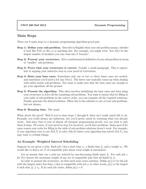
CSCI 280 Fall 2012
Dynamic Programming
Main Steps
There are 6 main steps to a dynamic programming algorithm-proof pair.
Step 1: Define your sub-problem. Describe in English what your sub-problem means, whether
it look like P (k) or R(i, j) or anything else. For example, you might write “Let S(k) be the
largest number of monkeys you can cram into k boxcars”.
Step 2: Present your recurrence. Give a mathematical definition of your sub-problem in terms
of “smaller” sub-problems.
Step 3: Prove that your recurrence is correct. Usually a small paragraph. This is equivalent
to arguing your inductive step in your proof of correctness.
Step 4: State your base cases. Sometimes only one or two or three bases cases are needed,
and sometimes you’ll need a lot (say O(n)). The latter case typically comes up when dealing
with multi-variate sub-problems. You want to make sure that the base cases are enough to
get your algorithm off the ground.
Step 5: Present the algorithm. This often involves initializing the base cases and then using
your recurrence to solve all the remaining sub-problems. You want to ensure that by filling in
your table of sub-problems in the correct order, you can compute all the required solutions.
Finally, generate the desired solution. Often this is the solution to one of your sub-problems,
but not always.
Step 6: Running time. The usual.
What about the proof? Well if you’ve done steps 1 through 6, there isn’t really much left to do.
Formally you could always use induction, but you’d pretty much be restating what you already
wrote. And since that is true of almost all dynamic programming proofs, you can stick to just
these 6 steps. Of course, if your proof in step 3 is incorrect, you’ll have problems. Same goes if for
some reason your order for filling in the table of sub-problem solutions doesn’t work. For example,
if your algorithm tries to use S(3, 7) to solve S(6, 6) before your algorithm has solved S(3, 7), you
may want to rethink things.
An Example: Weighted Interval Scheduling
Suppose we are given n jobs. Each job i has a start time s i , a finish time f i , and a weight w i . We
would like to find a set S of compatible jobs whose total weight is maximized.
Let us assume that our n jobs are ordered by non-decreasing finish times f i . For each job i,
let S(i) denote the maximum weight of any set of compatible jobs that all finish by f i .
In order to present the recurrence, we first need some extra notation. Define p(j) to be the job
with the largest index less than j that is compatible with job j; in other words, p(j) is the largest
k such that f k ≤ s j . If no such job exists, define p(j) = 0.

Our recurrence is S(i) = max{S(i − 1), w i + S(p(i))}.
To prove this is correct, consider the optimal solution for S(i). There are two cases: either job
i is used in the solution for S(i), or it is not.
case 1: If i is not used in the optimal solution for S(i), then the maximum-weight set of compatible
jobs among jobs 1 through i is just the maximum-weight set of compatible jobs among jobs
1 through i − 1; by definition, this is S(i − 1).
case 2: If i is used in the optimal solution for S(i), then since jobs p(i)+1 through i−1 all conflict
with job i, the remaining jobs selected for S(i) are drawn from 1 through p(i). Removing i
from the optimal solution for S(i) yields a compatible solution on jobs 1 . . . p(i). So by the
optimality of S(p(i)), S(i) − w i ≤ S(p(i)). But similarly, adding job i to S(p(i)) is (by the
definition of p(·)) compatible, and only uses jobs up through i. Hence S(i) − w i ≥ S(p(i)).
Therefore S(i) = w i + S(p(i)).
Finally, since S(i) is a maximization, the larger of these two cases is the weight of S(i).
As base cases, we define S(0) = 0 and S(1) = w 1 . This produces the following algorithm.
sort jobs by increasing finish times
compute function p(i) for i from 1 to n
set S(0) = 0 and S(1) = w 1
for i from 2 to n do
set S(i) = max{S(i − 1), w i + S(p(i))}
end for
return S(n)
Sorting takes O(n log n) time. The computation of p(i) can clearly be done in O(n 2 ) time; if
we want to do better, we can either binary search for each i, or all p(i) values can be computed
in a single pass if we have already created a second list of jobs sorted by increasing start times.
Finally, the main loop is linear; therefore the total running time is O(n log n).
Note that we computed the value of an optimal schedule, but not the schedule itself. To
actually compute the actual schedule, we have a few options. One is to use the computed values
S(i) to reverse engineer an optimal set A of jobs to select. Alternatively, we can change the
algorithms so we build lists as we go:
sort jobs by increasing finish times
compute function p(i) for i from 1 to n
set S(0) = 0 and S(1) = w 1
set A(0) = ∅ and A(1) = {1}
for i from 2 to n do
if S(i − 1) > w i + S(p(i)) then
set A(i) = A(i − 1) and S(i) = S(i − 1)
else
set A(i) = {i} ∪ A(p(i)) and S(i) = w i + S(p(i))
end if
end for
return A(n)
This version of the algorithm now requires O(n 2 ) space, since for each index we store a set of jobs
(which may be as large as n). Can you see how to modify this so that it only uses O(n) space?