STRUCTURE AND ENVIRONMENT STRUCTURE AND ...

STRUCTURE AND 

ENVIRONMENT 

ARCHITECTURE, CIVIL ENGINEERING, ENVIRONMENTAL ENGINEERING AND ENERGY 

No. 4/2011 vol. 3 PL ISSN 2081-1500 

www.sae.tu.kielce.pl 

KIELCE UNIVERSITY OF TECHNOLOGY

Contents 

TOMASZ ARCISZEWSKI, JEFFREY RUSSELL 

CHANGE DEMANDS RENAISSANCE IN CIVIL ENGINEERING EDUCATION ................................................................................. 5 

PAWEŁ KOSSAKOWSKI 

LOAD–BEARING CAPACITY OF WOODEN BEAMS REINFORCED WITH COMPOSITE SHEETS ....................................................... 14 

IZABELA ANTCZAK, ANITA BANAŚ, IZABELA KAPUŚCIŃSKA 

THE USE OF THERMOVISION IN THE ESTIMATION OF THERMAL ENERGY LOSSES OF BUILDINGS .............................................. 25 

JOLANTA LATOSIŃSKA, ALICJA TURDAKOW 

THERMAL UTILIZATION OF MUNICIPAL SEWAGE SLUDGE – EXAMPLES OF POLISH SOLUTIONS ............................................... 31 


PROTECTION AGAINST NOISE IN THE EUROPEAN UNION – GENERAL REQUIREMENTS, 

AP-PLIED NOISE INDICATORS AND ASSESSMENT METHODS .................................................................................................. 38 

HOW TO PREPARE THE MANUSCRIPT .................................................................................................................................... 47 

THE REVIEW PROCESS ......................................................................................................................................................... 48

EDITORIAL BOARD 

Main Editor Jerzy Z. Piotrowski 

Editor Ludwik Śliwa 

Secretary of the Editorial Board Radosław Zaborek 

Sectional Editor STRUCTURE Zdzisława Owsiak 

Sectional Editor ENVIRONMENT Lidia Dąbek 

SCIENTIFIC BOARD 

Chairmanship Tomasz Kozłowski 

STRUCTURE 

Tomasz Arciszewski (USA), Lesław Brunarski, Go Iwahana (Japan), Marek Iwański, Zbigniew Kowal, Jozef Melcer (Slovakia), 

Michaił V. Nemchinov (Russia), Victor Proskuriakow, Zbigniew Rusin, Bohdan Rymaszewski, Wacław Seruga, 

Malgorzata Wilczkiewicz (USA) 

ENVIRONMENT 

Satoshi Akagawa (Japan), Elżbieta Bezak-Mazur, Dorota Chwieduk, Graham Herbertson (Scotland), Andrzej Kapłon, 

Andrzej Kuliczkowski, Janusz Łomotowski, Paweł Purgał, Leszek Radziszewski, Anatol Stroy (Ukraine), Maria Żygadło 

www.sae.tu.kielce.pl 

sae@tu.kielce.pl 

The quarterly printed issues of Structure and Environment are their original versions 

The Journal published by the Kielce University of Technology 

Faculty of Civil and Environmental Engineering 

PL ISSN 2081-1500 

© Copyright by Wydawnictwo Politechniki Świętokrzyskiej, 2011 

25-314 Kielce, al. Tysiąclecia Państwa Polskiego 7 

tel. 41 34 24 581 

www.tu.kielce.pl/organizacja/wydawnictwo

TOMASZ ARCISZEWSKI 

the Volgenau School of Information Technology and Engineering 

George Mason University 

tarcisze@gmu.edu 

JEFFREY RUSSELL 

College of Engineering, University of Wisconsin-Madison 

Russell@eng.wisc.edu 

CHANGE DEMANDS RENAISSANCE 

IN CIVIL ENGINEERING EDUCATION 

A b s t r a c t 

Much has been written about how the world has changed and continues to change at an incredibly rapid pace. Much has 

also been written about globalization, population demands, water quality, waste management, and many more of the issues 

that confront human kind throughout the world. It is not the authors’ purpose in this paper to repeat the familiar maxim: 

civil engineering education must change to meet the challenges of a rapidly changing world. Instead, the authors clarify the 

very real risks of the vectors of psychological inertia, and describe how systems analysis and the theory of inventive problem 

solving (TRIZ) justify substantive change in civil engineering education and how that could be accomplished. 

Keywords: civil engineering education, national and local needs, contradictions, systems analysis, TRIZ, evolution 

1. The Fluidity of Rapid Change Surrounds Us 

Civil engineering is undergoing rapid changes driven 

by globalization, growing environmental, safely and 

security concerns, population demands, the computer 

revolution, and by scientific advances in fields such 

as biotechnology, materials science, nanotechnology, 

and many more. Obviously, such changes demand 

that students acquire more knowledge than in the 

past, not only traditional engineering knowledge 

based in science and math, but also new knowledge 

that encompasses emerging domains in science and 

engineering and knowledge in critical areas such as 

communications, leadership, business management, 

marketing, and the political process. 

Furthermore, students need to learn how to develop 

novel designs, and that is absolutely necessary to 

maintain and expand our competitive advantage 

with respect to other countries and to be adequately 

prepared to meet coming professional challenges. 

Therefore, there are strong national needs to expand 

and enhance civil engineering education (CEE), 

including educating innovators, i.e. civil engineers 

with knowledge and skills necessary to develop novel 

designs, which might be potentially patentable. 

Over the last 60 years a strong national trend has 

taken place in reducing the number of credit hours 

required for a BS degree in civil engineering. Presently, 

the US average is as little as 125 credit hours, down 

from 135 credit hours only 20 years ago. This trend is 

driven primarily by state funded universities bowing to 

political pressures to reduce the cost of undergraduate 

education and to ensure that BS students graduate in 

four years. Unfortunately, private universities follow 

this trend mostly to remain competitive. 

Today, civil engineering educators struggle with 

the obvious contradiction between the national and 

local and state levels needs. The traditional national 

needs mean expansion of the CEE and a broad-based 

approach to moving forward. Whereas the local needs 

are much more often focused on the here and now, 

attuned to local and community politics and economic 

conditions; often resulting in efforts to reduce the 

breadth and depth of CEE. This contradiction cannot 

be eliminated through quantitative changes within the 

existing paradigm. Our hypothesis is that the existing 

situation requires a constant evolution of CEE. 

However, this will be insufficient and bold action and 

qualitative, or paradigmatic, changes are required in 

addition to constant minor quantitative improvements. 

The objective of this paper is to present a theoretical 

justification for the constant evolution of CEE and for 

paradigmatic changes as well as to demonstatrate how 

such changes could be accomplished. The authors have 

developed the paper within the context of Systems 

5

Tomasz Arciszewski, Jeffrey Russell 

Science and of the Theory of Creative Problem Solving 

(TRIZ), which is also based on systems analysis. The 

fact is, the fluidity of rapid change surrounds us. As 

a profession, we must embrace it because time and 

change only move in one direction. 

2. Escaping the Vector of Psychological Inertia 

We are humans and our behavior, including 

professional behavior, is strongly affected by the 

ʺVector of Psychological Inertiaʺ (VPI) [1], [4], [5], 

[7]. Put in simple terms, as we operate within the 

VPI we are comfortable it what we know, in our 

given perspective, and in the manner and methods 

we employ to achieve our goals. It is understood as a 

natural human tendency to focus on known solutions in 

our own domain and to be extremely reluctant to seek 

solutions outside of our domain. Such an approach 

provides a psychological explanation as to why it is 

so difficult to think ʺoutside the boxʺ and why so often 

we follow the vector of psychological inertia (rooted in 

our experience) instead of following the evolution of 

the system being considered (See the next section for 

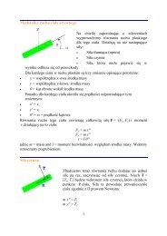
more on the evolution of engineering systems) (Fig. 1). 

The vector of psychological inertia affects even 

talented inventors, who usually invest a lot of time and 

effort investigating local lines of evolution within their 

domain instead of initiating a process directly leading 

to the desired solution and based on the general patterns 

of evolution [1], [4], [5], [7], [11], [17]. 

The vector of inertia accompanies many practices 

and professions, in nearly every undertaking that 

comprises the human experience – from ancient times to 

contemporary life. This does not mean it is a good thing, 

for the vector of inertia impedes progress whether one 

considers the development of the latest styles of mobile 

telephones, or the current crisis facing the newspaper 

industry. The vector of inertia is characterized by an 

over-reliance on routine, and a failure to respond to 

external conditions and circumstances. 

Consider the example of Nokia, the world’s largest 

mobile phone maker. Five years ago Nokia paid a 

heavy price for being slow to adapt to consumer 

demand for new clamshell telephone handsets. At 

the time, Nokia saw its market share dip significantly 

and reported a 2% drop in first quarter profits. Major 

competitor Samsung Electronics recorded soaring 

profits, and an increase of 178% in a year-over-year 

comparison, marking the company’s best quarter ever. 

In some instances it takes a full-blown crisis to jumpstart 

an industry and to elevate it beyond the vector 

of inertia. Such a crisis is confronting the newspaper 

industry as of this writing. The business model upon 

which most daily and weekly newspapers were 

founded has become obsolete, advertising revenues 

have declined significantly as well as levels of 

readership. Readers are flocking to internet news sites 

where they can acquire the news they need for free, and 

newspapers are scaling back, cutting staff, ceasing to 

publish in print and maintain an online presence only, 

and devising new business models in which readers 

will be encouraged to pay for content. 

Fig. 1. The Vector of Psychological Inertia 

6

CHANGE DEMANDS RENAISSANCE IN CIVIL ENGINEERING EDUCATION 

The Internet and the general and wide spread 

availability of information at any time is one reason 

why newspapers have been struggling to survive. 

The organizational and managerial recipes that they 

have followed have become outdated, and lead to the 

growth of strategic inertia – the level of commitment 

to current strategy. As Wright et al. [16] has noted, 

ʺAn organization’s strategic decision-making must 

retain or improve the organization’s alignment with 

the external world. In other words, (management) 

recipes should not be routinely followed and should 

be changed altogether when appropriateʺ. 

Reluctance to evolve CEE is well known, but 

mechanisms behind it are not fully understood. This 

often leads to emotional arguments, which create 

even more resistance to change. We believe that 

understanding the phenomenon in objective and 

scientific terms will help us improve the situation. The 

impact of the vector of psychological inertia is often 

harmful because it delays progress, as we discussed it 

earlier in the areas of communication and mass media. 

In CEE, there are many examples of how the vector 

of psychological inertia set back necessary changes, 

such as delaying the elimination of outdated courses, 

reviewing the curriculum as a system as opposed to a 

group of courses, or the introduction of new courses. 

For example, when the evolution of required and 

elective courses at the Civil, Environmental, and 

Infrastructure Engineering Department at George 

Mason is considered, the vector of inertia in action 

can be easily observed. About 15 years ago a novel 

required course on computer graphics in civil 

engineering was introduced, ENGR 183 ʺEngineering 

Computer Graphicsʺ. Its major focus was on teaching 

practical AutoCAD skills in the context of civil 

engineering applications. Today, many students take 

computer graphics courses at the high school and/or 

learn AutoCad during their summer internships, but 

the course is still offered. Even more, about a year ago, 

Dr. Michael Casey introduced a new elective course 

CEIE 472, ʺBuilding Information Management.ʺ It 

represents the state of the art in the area of virtual 

design and construction and obviously includes the 

use of computer graphics and the AutoCAD but the 

old course is still offered and has not been modified to 

reflect the introduction of the new course. 

When CEE is considered, we must be aware of the 

existence of the vector of psychological inertia and 

try to deliberately minimize its impact. If we fail to 

do so, we will make only small quantitative changes 

within our domain, without the benefit of knowledge 

beyond the realm of civil engineering. We must always 

remember that with improvement comes added value. 

3. New Approaches Hold Promise and Potential 

Systems Analysis 

In the late 1940’s, cybernetics emerged as a 

discipline dealing with abstract models of purposeful 

living organisms, artificial objects, or processes 

in nature and engineering, which were called 

ʺsystems modelsʺ, or simply ʺsystemsʺ. Systems 

analysis created a revolution in our understanding 

of nature and engineering, revealing many common 

behavioral patterns and improving our ability to 

analyze and predict behavior of various systems. It 

allows the development of an abstract understanding 

of behavior of a given system in the context of its 

feedback with the environment in which it operates, 

including its past, present, and future responses 

(feedback) to the evolving environment. Presently, 

Systems Engineering (SE), a discipline descendent 

from cybernetics, is recognized as an engineering 

science and is taught to SE students, and also to 

civil engineering students. The recently updated and 

published Civil Engineering Body of Knowledge for 

the 21 st Century [6] explicitly recognizes systems 

analysis as an appropriate and recommended 

analytical method for civil engineers. Systems 

analysis, and particularly the concept of a complex 

adaptive system provide an excellent understanding 

of CEE in general and objective systems terms. 

Theory of Inventive Problem Solving (TRIZ) 

The history of TRIZ spans more than 60 years, two 

continents, and three political systems. Ultimately, 

TRIZ is a result of efforts of a large group of 

talented engineers and inventors. TRIZ (a Russianbased 

acronym for the Theory of Inventive Problem 

Solving) can be considered as a knowledge system. It 

contains a class of inventive problem solving methods 

and a body of abstract engineering knowledge, 

necessary and sufficient to conduct the generation of 

inventive design concepts (inventions) in the majority 

of engineering domains. TRIZ is based on three 

fundamental assumptions. 

The first assumption is that the generation of 

inventive design concepts in a specific engineering 

domain can be conducted using inventive knowledge 

acquired from engineering patents awarded in many 

engineering domains and in various countries over a 

long time period, and from other traditional sources 

of engineering knowledge. Inventive knowledge can 

7


be represented as heuristics (heuristic directives) 

formulated for various specific situations. Such 

heuristics are called ʺPatterns of Inventionʺ. 

The second fundamental assumption deals with the 

evolution of engineering systems, built and abstract. 

This assumption maintains that when evolution of 

engineering systems over a time period is considered, 

they evolve not randomly, but according to objective 

patterns, called ʺPatterns of Evolutionʺ. Patterns of 

Evolution were discovered by Altshuller and other 

TRIZ researchers through learning from patents and 

from the history of engineering [1], [5], [11], [17]. 

There are nine patterns of evolution (Introduced in 

Section ʺFive Perspectivesʺ). 

Finally, Altschuller has assumed that any 

inventive problem (i.e. problem requiring a novel 

and potentially patentable solution) requires 

elimination of contradictions, technical and physical. 

A technical contradiction is an interrelated pair of 

technical (abstract) contradictory characteristics of 

an engineering system. For example, rigidity versus 

weight. A physical contradiction occurs when a given 

physical characteristic of an engineering system 

should increase and decrease to satisfy different 

requirements. For example, the depth of a reinforced 

concrete beam should be maximized to increase 

rigidity and minimized to reduce weight. Typically, a 

physical contradiction results from a technical one. In 

the example, the technical contradiction is obviously 

rigidity versus weight. 

There are many publications on TRIZ available in 

English, for example [2], [5], [7], [10], [12-15], [17]. 

4. Assumptions 

Our analysis of CEE has been based on several 

assumptions, provided in this section. 

• Our society constantly evolves, creating evergrowing 

demands for CEE. 

• Globalization of the civil engineering market is a 

fact and competition is driven primarily by costs, 

quality, and novelty of designs and services. 

• Traditional CEE offered in Europe and in many 

developing countries, particularly India, is much 

more extensive than in the US and often of 

comparable or better quality. 

• The extent of CEE offered in this country has 

gradually been reduced (From 135 credit hours 

required 20 years ago to an average 125 today with 

many programs requiring only 120 hours). 

• American civil engineers cannot win in the 

global competitive market based only on cost and 

quality. They have to develop an innovation-based 

competitive advantage. Clearly, we won’t win on 

numbers alone and we have to compete with better 

solutions and better ideas. 

• CEE is the key to the future of our profession and 

in fact the key to the future of our nation. 

• CEE is a system operating in an evolving 

environment. 

5. Five Perspectives 

Evolutionary Perspective 

In accordance with TRIZ (see the Theory 

of Inventive Problem Solving), the evolution 

of engineering systems is driven by objective 

evolutionary mechanisms, called ʺPatterns of 

Evolutionʺ. These patterns are valid in all areas of 

engineering, including civil engineering education 

and practice. Many studies, going back to the late 

1940’s, of the tens of thousands of engineering patents 

in many countries revealed nine patterns of evolution 

of engineering systems [1], [5], [11], [17], including: 

1. System evolution based on S-curve. 

2. Resources utilization. 

3. Uneven development of system elements. 

4. Increased system dynamics. 

5. Increased system controllability. 

6. Increased complexity followed by simplification. 

7. Matching and mismatching of system elements. 

8. Transition to the micro-level and increased use of fields. 

9. Transition to decreased human involvement. 

All these patterns are relevant to the evolution of 

CEE, but our focus is only on the first pattern, which 

is explained here. It says that all engineering systems 

evolve over their life period following an S-curve 

pattern when a relationship between a specific 

system’s characteristic and time is considered. That 

means that during a life cycle of a given system, several 

distinct evolutionary patterns can be distinguished, 

each of a different nature. They include the periods 

of childhood (slow growth), growth (rapid growth), 

maturity (no growth), and decline (negative growth), 

as shown in Figures 2 and 3. More importantly, this 

pattern also means that each engineering system has 

its life cycle and when it is completed (the system 

reaches its decline stage) it must be replaced by a 

system based on a different set of assumptions, on 

a different paradigm. For example, when planes are 

considered, there are separate S-curves for propellerdriven 

planes, turbo-propeller planes, and jet planes. 

We have a family of S-curves. 

8


Fig. 2. System Evolution: S-Curve 

Fig. 3. S-Curve in Action 

Fig. 4. Family of S-curves 

In general, evolution of a system can be presented 

as a class of S-curves. Each separate curve represents 

evolution within a given paradigm or a quantitative 

evolution. A transition between curves represents 

a paradigm change, a qualitative change, or a 

revolutionary change. 

In the area of CEE education, we can distinguish at 

least two paradigms, each with its separate S-curve 

when the success of our profession is considered, 

measured by our prestige, salaries, attractiveness 

to the best and brightest students, and other factors. 

Until about a hundred years ago, civil engineering 

education was based on the ʺmaster-apprentice 

paradigmʺ. Throughout many centuries of practice, 

educating engineers was more an art than a science. 

Such teaching was a combination of rote learning 

(memorization of known facts and heuristics) and of 

acquisition of knowledge through learning by example 

and hands-on experience. An apprentice would 

produce abductively new hypotheses (plausible rules 

or heuristics) describing his/her recent experience and 

inductively verify them in the context of examples 

from experience. In this way, an apprentice would 

acquire not only new knowledge but would also learn 

how to conduct induction and how to abductively 

generate hypotheses, or new ideas about engineering 

(See Glossary for our definitions of induction and 

abduction). Abduction, or inference to the best 

explanation is the key to human learning and creativity. 

Therefore, the master-apprentice model of education 

produced not only civil engineers but also leaders 

and inventors. Unfortunately, it was time-consuming, 

costly and could produce only a limited number 

of engineers. Table 1 illustrates civil engineering 

knowledge associated with this paradigm [9]. 

At the end of the 19th Century, progress in science, 

particularly in mathematics and physics, changed the 

dynamics of engineering education. These changes 

resulted in a growing trend to teach engineering 

as a science, to focus on the ʺscientificʺ, or the 

mathematical foundation of engineering. In this way, 

a ʺscientific paradigmʺ emerged and the focus of 

Table 1. Civil Engineering Knowledge: Master-Apprentice Paradigm ([9], accepted) 

Categories 

Scientific Engineering Civil Engineering Domain - specific 

Factual knowledge Facts XXX 

Models 

Procedural knowledge Deterministic procedures 

Heuristic procedures 

XXX 

Rules 

Decision rules 

Heuristics 

XXX 

9


engineering education changed. Instead on building 

a qualitative/holistic understanding of engineering 

based on heuristics, as before, the focus shifted to 

acquiring formal knowledge, an inflexible knowledge 

system. As a result, deduction, the process of deriving 

the consequences of what is assumed, became the 

main form of reasoning at the expense of abduction. 

Deduction allows verification of a given hypothesis in 

the context of existing knowledge, but it cannot be used 

to generate a new hypothesis. Thus, an engineer trained 

mostly in deduction is an excellent follower, focused on 

satisfying existing regulations and rules of practice but 

unprepared to take the lead and to produce the new ideas 

that are critical to innovation and progress. The civil 

engineering knowledge associated with this paradigm is 

shown in Table 2. There is a significant difference with 

respect to the knowledge associated with the Master – 

Apprentice Paradigm ([9], accepted). 

Today, the primary focus of civil engineering 

education is on analysis, on building quantitative 

understanding and numerical optimality, as it is in 

science. This analysis is mostly based on deduction. 

Civil engineering knowledge is still partially heuristic, 

although over the last century it has been supplemented 

by all kinds of mathematics- and physics-based theories, 

including complex mathematical models. We are all 

proud that civil engineering has become a science, but 

at the same time we are becoming painfully aware that 

the price for this progress is the loss of our creativity 

and excessive focus on the quantitative aspects of our 

profession. This shift from art to science has ultimately 

led to civil engineers losing their leadership and 

being inadequately prepared to deal with the complex 

challenges of the 21st century. 

The scientific paradigm in civil engineering is today 

simply insufficient. It has to be critically examined 

and replaced by a new paradigm preserving its allobvious 

advantages but at the same time providing 

knowledge, skills, and styles necessary for today. In 

the context of the S-curve Pattern of Evolution, the 

present evolution of CEE reached a period of decline 

and a paradigmatic change is a must. 

Contradictions Analysis 

The identified contradiction between national and 

local needs in CEE can be presented in the form of both 

technical and physical contradictions in accordance with 

TRIZ [1], [5]. Such formulations provide additional 

insight and allow using TRIZ ʺInventive Principlesʺ to 

find novel ways to eliminate the contradiction, although 

this is not the focus of this paper. 

Our contradiction can be formulated as a technical 

contradiction between the complexity of a system 

and its speed. In this case, the complexity of CEE 

can be considered as a feature measured by the 

number of courses and their differentiation, and the 

speed of its delivery can be considered as a feature 

measured by the number of years necessary to deliver 

all courses required for graduation. TRIZ provides 

three inventive principles, which can be used to 

eliminate this technical contradiction. They include 

those of ʺPrior Actionʺ, (No. 10), ʺReplacement 

of a Mechanical Systemʺ, (No. 28), and ʺRejecting 

and Regenerating Partsʺ, (No. 34). These inventive 

principles can be used to reinvent CEE and they 

are not fully described in this paper. However, their 

initial interpretation in the context of CEE provides 

a glimpse of opportunities for civil engineering 

educators willing to accept and take bold action. 

The principle ʺPrior Actionʺ can be interpreted in 

two ways [15]. 

1) Carry out all or part of the required action in advance. 

2) Arrange objects so they can go into action in a 

timely manner and from a convenient position. 

The first principle recommends a pre-civil 

engineering education understood as a required 1-4 

year program to be taken BEFORE entering a civil 

engineering program. The second principle can be 

interpreted as a recommendation to divide incoming 

civil engineering freshmen into several cohorts in 

accordance with their knowledge and analytical 

intelligence, as measured, for example, by IQ. Each 

cohort would be provided an appropriate instruction 

and allowed to take demanding courses when ready. 

Table 2. Civil Engineering Knowledge: Scientific Paradigm ([9], accepted) 

Categories 

Scientific Engineering Civil Engineering Domain - specific 

Factual knowledge Facts XXX XXX XXX XXX 

Models XXX XXX XXX XXX 

Procedural knowledge Deterministic procedures XXX XXX XXX XXX 

Heuristic procedures 

Rules Decision rules XXX XXX XXX XXX 

Heuristics 

10


The principle ʺReplacement of a Mechanical 

Systemʺ can be interpreted as substituting traditional 

testing laboratories and facilities by virtual ones. 

More generally, this principle also means using distant 

learning and an all IT-based means of instruction. 

There are two interpretations of the inventive principle 

ʺRejecting and Regenerating Partsʺ: 

1) After it has completed its function or become 

useless, reject or modify an element of an object. 

2) Immediately restore any part or an object, which is 

exhausted or depleted. 

In the first case, when a student fails a prescribed 

number of exams, he/she is immediately expelled 

from a program or offered a number of required noncredit 

courses to improve his/her performance. The 

second heuristic can be interpreted as conducting 

constant performance monitoring and immediate 

feed back in the form of individual counseling and 

tutoring to failing students. 

Our fundamental contradiction can be formulated 

as a physical contradiction when the number 

of courses in civil engineering education is 

considered. This number must be increased and 

reduced at the same time. Both interpretations of 

this contradiction clearly demonstrate that it cannot 

be simply eliminated through quantitative changes 

within a given paradigm. This elimination requires 

a qualitative, or paradigmatic change, in addition to 

obvious quantitative improvements. 

Complex Adaptive Systems Perspective 

CEE can be considered as a Complex Adaptive 

System, which has three unique features: 

• It is complex and has a sufficient number of 

subsystems and components allowing changes in 

its structure and components 

• It has an ability to adapt, to change its structure and 

components as feedback to the changing environment 

• It has an ability to learn, to acquire knowledge 

through inductive learning about its behavior and 

environment 

In general terms, a complex adaptive system can be 

described as a learning system with an ability to undergo 

both qualitative/structural and quantitative/component 

level changes in response to its changing environment. 

The still prevailing approach to civil engineering 

education is non-systemic. When CEE in a given 

department is considered (a specific program), it 

is usually assumed that a selected combination of 

courses is optimal and frozen in time. In addition, 

CEE usually operates only in the context of a 

given university and of a local community of civil 

engineering practitioners, no matter how society, 

engineering, and the entire world evolve. However, 

when it is considered as a complex adaptive system, an 

entirely new understanding of the situation emerges. 

The environment of a given complex adaptive system, 

in our case a program offered by a given department, 

can also be considered as another complex adaptive 

system. It has a number of subsystems, including: 

• An educational subsystem with coursework 

offered through civil engineering departments in 

this country and abroad 

• A social system with national and international 

components 

• A science subsystem representing national and 

global science and its evolution 

• A cultural subsystem 

• A political subsystem 

All these subsystems evolve, most likely following 

their own separate and unique lines of evolution. As 

a result, the behavior of the environment cannot be 

entirely predicted and it produces often unexpected 

and undesired inputs to the education system, forcing 

it to evolve constantly and to change its behavioral 

patterns. Such unpredictable and unexpected 

behavior is called ʺemergent behaviorʺ and must be 

recognized as a real possibility in the case of CEE. 

Usually, we do not immediately know how to comply 

with an emergent behavior, but being aware of the 

possibility of its occurrence is a proactive way of 

being responsible and concerned about the future. 

When the environment of CEE is considered as 

a complex adaptive system, the traditional static 

understanding of CEE is simply inadequate and most 

likely wrong. Using it potentially may be harmful 

because it offers a simplistic understanding of the 

situation and puts its users in a disadvantageous 

position with respect to educators making decisions 

based on the complex adaptive system model of CEE. 

Globalization Perspective 

US civil engineering companies are involved in 

a fierce competition for market share – indeed for 

survival – with competitors from many countries that 

offer significant labor cost advantages. Changing 

the course of US civil engineering education to 

emphasize creative problem solving will create a 

novelty-driven competitive advantage. In addition, 

novel engineering solutions that directly address the 

specific challenges of a project can often produce 

significant cost savings [8]. 

11


Today, globalization of civil engineering work is an 

objective trend driven by costs, by the high quality 

of traditional civil engineering education in many 

developing countries, and by progress in information 

technology that has made outsourcing not only 

feasible but also inexpensive. Such a trend cannot 

be simply reversed; the proportion of engineering 

work being outsourced will continue to increase. The 

obvious consequence of such outsourcing will be 

reduced demand within the US for civil engineering 

services. Unfortunately, that may lead to the mass 

elimination of civil engineering jobs in this country, 

especially those related to routine work. 

In practical terms, outsourcing can be offset, at least 

partially, only if a new demand for civil engineering 

services is created. Such demands will be driven by 

novel solutions and products, clearly the result of fresh 

thinking, creativity and unrelenting innovation. This 

work will have to utilize state-of-the-art knowledge 

and will require engineering creativity. Innovation and 

creativity combined with the highest levels of expertise 

will be the added value that prevents non-routine work 

from being outsourced, at least as long as this country 

maintains its competitive advantage in research and 

development and uses and applies recently acquired 

knowledge in a creative way to produce novel solutions. 

Legacy Perspective 

The future of civil engineering in the US depends on the 

quality of our successors. If high school students know 

that civil engineers are only followers and do mostly 

highly repetitive, routine work, the best, brightest, and 

most talented students will never enter civil engineering 

programs or will soon transfer to other disciplines such 

as electrical or computer engineering. Unfortunately, 

this is more than a pessimistic prediction; it is a troubling 

trend occurring in many civil engineering programs. 

High salaries and job security are not enough to 

attract the brightest students. They are looking not only 

for material benefits but also for emotional awards, 

including novelty and excitement. Today there is 

not much excitement in civil engineering education 

and practice. The still strong enrollment numbers 

provide only false comfort. These numbers are more 

a reflection of the Internet bubble burst and of a still 

relatively strong demand for civil engineers than of 

the intellectual attractiveness of our profession. Also, 

we should be aware that the ongoing real estate crisis 

has already reduced the demand for civil engineers 

specializing in land development and that may 

lead to declining enrollments. If we are looking for 

permanent solutions, we need to restore the past glory 

of civil engineering, and the excitement of being a 

civil engineer must be recreated. 

Reconnecting civil engineering with creativity – 

with doing non-routine work – generates excitement. 

We can transform civil engineering education by 

teaching students how to become creative problem 

solvers, inventors leading the generation of novel 

solutions that contribute to the fundamental needs of 

society and advance our civilization. 

6. Conclusion – A Storied Past. A Boundless Future 

We live in a rapidly changing world in which 

progress in information technology and computing 

drives significant changes in science and technology, 

fuels globalization, and changes our society. In this 

context, for our profession to survive and especially 

to grow, CEE must continually evolve and never stop 

re-inventing itself. The five perspectives on CEE 

evolution noted earlier clearly explain why such 

evolution is simply a must. 

CEE is a complex adaptive system, in constant 

motion. However, most of this consists of quantitative, 

gradual improvements without structural change. 

From time to time, environmental changes simply 

force civil engineering programs to adapt through 

qualitative changes requiring significant structural 

changes like the introduction of new outcomes, 

elimination of existing outcomes, changes in the 

required levels of performance, and significant 

changes in course offerings. 

The marketplace demands that we continue to push 

for reform. As a profession, we must meet future 

challenges with the best ideas, and at the lowest 

cost. That is the key to competitive advantage in a 

global market. ʺConventional approaches to such 

unconventional demands simply will not get the job 

done. Systematic innovation in products and processes 

is an imperative for competitive leverageʺ [12]. 

Today, we have to recognize that the evolution 

of CEE must become a part our activities and that 

championing continual changes and improvements is 

simply a part of our responsibilities to society and to 

our students. Change requires time and effort and the 

vector of inertia is always hovering about. It is time 

for us to realize that we are too great a profession 

to limit ourselves to small dreams, and inaction is 

simply not an option. The stakes are just too high. 

Glossary 

• A system is a set of interrelated objects (subsystems) 

working together to provide a specific function, 

12


which could not be provided by a single object or 

any subset of objects belonging to a given system. 

• A complex adaptive system is a system with three 

major unique features: 

– It is complex, and has a sufficient number of 

subsystems and components allowing changes 

in its structure and components 

– It has an ability to adapt, to change its structure 

and components as feedback to the changing 

environment 

– It has an ability to learn, to acquire knowledge 

through inductive learning about its behavior 

and environment 

• Deduction is a form of logical reasoning in which 

existing knowledge and new data are used to verify 

hypothesis about data 

• Induction is a form of logical reasoning in which 

existing knowledge and new data in the form 

of examples are used to verify new hypothesis 

about data. 

• Abduction is a form of logical reasoning in 

which existing knowledge and new data are used 

to generate new hypothesis about data, which, if 

verified by deduction or induction, can be used to 

expand existing knowledge. 

• Contradiction: ʺEvery great invention (a 

creative design concept) is the result of resolving 

a contradictionʺ [1]. Therefore, generation of 

inventive design concepts involves the elimination 

(resolution) of contradictions. There are two types 

of contradictions: technical and physical. 

• Technical Contradiction is an interrelated pair of 

technical (abstract) contradictory characteristics 

of an engineering system. For example, rigidity 

versus weight. 

• Physical Contradiction occurs when a given 

physical characteristic of an engineering system 

should increase and decrease to satisfy different 

requirements. For example, the depth of a 

reinforced concrete beam should be maximized to 

increase rigidity and minimized to reduce weight. 

• Inventive Principles are heuristics acquired from 

patents and other sources. They are intended for 

the elimination of technical contradictions in the 

process of creative design concepts generation. 

In the early 1970s, Altshuller created the set of 40 

inventive principles. Today, there over 400 inventive 

principles (called ʺOperatorsʺ in I-TRIZ) available. 

• Patterns of Evolution are objective patterns describing 

changes in an engineering system over a long time 

period. They are valid in all engineering domains. 

References 

[1] Altshuller G., The Innovation Algorithm, Moskowskii 

Rabochii Publishing House, (in Russian), 1969. 

[2] Altshuller G., Creativity as an Exact Science. Gordon 

and Breach, Science Publishers, Inc., 1984. 

[3] Altshuller G., And Suddenly the Inventor Appeared, 

TRIZ, the Theory of Inventive Problem Solving, Technical 

Innovation Center, Worcester, Massachusetts 1996. 

[4] Altshuller H., Boris Zlotin B., Alla Zusman A., 

Philatov V., Searching for New Ideas: From Insight to 

Methodology; The Theory and Practice of Inventive 

Problem Solving, Kishinev: Kartya Moldovenyaska, 

Publishing House, (In Russian), 1989. 

[5] Altshuller G., The Innovation Algorithm, Technical 

Innovation Center, Worcester, Massachusetts. 1999. 

[6] American Society of Civil Engineers. Civil 

Engineering Body of Knowledge for the 21st Century, 

Preparing the Civil Engineer for the Future, Second 

Edition, 2008. 

[7] Arciszewski T., ARIZ 77 – An Innovative Design 

Method, Journal of Design Methods and Theories, 

22(2), 796-820, 1988. 

[8] Arciszewski T., Civil Engineering Crisis, ASCE 

Journal of Leadership and Management in 

Engineering, 6(1), 26-30, 2006. 

[9] Arciszewski T., Harrison C., Successful Civil 

Engineering Education, the ASCE Journal of 

Professional Issues in Engineering Education and 

Practice, accepted, 2008. 

[10] Clarke D., TRIZ: Through the Eyes of an American 

TRIZ Specialist, Ideation, 1997. 

[11] Clarke D., Strategically Evolving the Future: Directed 

Evolution and Technological Systems Development, 

special double issue, ʺInnovation: the key to Progress 

in Technology and Society,ʺ Arciszewski, T., (Guest 

Editor), Journal of Technological Forecasting and 

Social Change, North-Holland, 64(2-3), 133-153. 2000 

[12] Fey V., Rivin E., Innovation on Demand: New Product 

Development Using TRIZ, Cambridge University 

Press, 2005. 

[13] Kaplan S., Introduction to TRIZ, The Russian Theory of 

Inventive Problem Solving, Ideation International, 1996. 

[14] Orloff M.A., Inventive Thinking through TRIZ, 

Springer, 2003. 

[15] Terninko J., Zusman A., Zlotin, B., Systematic 

Innovation, An Introduction to TRIZ, St. Lucie Press, 

1998. 

[16] Wright G., van der Heijden K., Bradfield R., Burt G., 

Cairns G., The Psychology of Why Organizations Can 

Be Slow to Adapt and Change, Journal of General 

Management, 29(4), 21-36, 2004. 

[17] Zlotin B., Zusman A., Directed Evolution: Philosophy, 

Theory, and Practice, Ideation International, 2006. 

13


Kielce University of Technology 


al. Tysiąclecia Państwa Polskiego 7 

25-314 Kielce, Poland 

e-mail: kossak@tu.kielce.pl 

LOAD–BEARING CAPACITY OF WOODEN BEAMS 

REINFORCED WITH COMPOSITE SHEETS 


The paper presents preliminary data on load-bearing capacity of wooden beams reinforced with composite sheets subjected 

to static bending. The tensile part of beams was reinforced with composite sheets from S&P Clever Reinforcement AG. 

Glass sheet S&P G-Sheet AR 50/50, aramid sheet S&P A-Sheet 120/290 and carbon sheet S&P C-Sheet 240/400 were 

used. Basing on the tests results it can be concluded that the load-bearing capacity rose in the range 20-48% due to the 

application of one-layer reinforcement. The obtained results are promising and indicate future research possibilities 

especially with the use of carbon sheets. 

Keywords: wood, wooden beams reinforcement, composites, composite sheet 

1. Introduction 

Over the years composites have become basic 

materials used in construction engineering to 

strengthen elements. They are most widely applied to 

reinforce concrete and reinforced concrete structures, 

while less masonry and wood structures. Composites 

are also used to reinforce construction elements 

from other materials, including wood and wood-like 

materials. 

Wood is reinforced mainly with composite laminates. 

Fewer cases deal with sheets. Due to a small number 

of studies on wood reinforcement with composite 

sheets, this issue is still being investigated in Poland 

and abroad, eg. [1, 2]. 

The paper presents the problem of wooden beams 

reinforced with composite sheets. The preliminary 

strength test results have been presented aimed at 

determining a degree of reinforcement with glass, 

aramid and carbon fibers. 

2. Strength test of beams reinforced with composite 

sheets 

The strength tests covered static bending of wooden 

beams without reinforcement and reinforced with 

Table 1. Parameters of the composite sheet with glass fibers S&P G-Sheet AR 50/50 [6] 

Elastic modulus [kN/mm 2 ] 65 

Tensile strength (virgin filament) [N/mm 2 ] 3000 

Sheet weight (total 350 g/m 2 ) [g/m 2 ] 

175 in both directions 

Density [g/cm 3 ] 2.68 

Elongation at rupture [%] 4.3 

Design thickness (fibre weight/density) [mm] 0.065 

Theoretical design cross-section 1000 mm width [mm 2 ] 

65 (fibre area only/each direction) 

Reduction factor for design (manual lamination / UD sheet) 1.4 (recommended by S&P) 

Tensile force of 1000 mm width for design [kN] 

(65 × 3000)/1.4 = 139.3 each direction 

– Explosion protection 

Application: 

– Reinforcing of masonry or historic buildings 

– Seismic retrofitting 

14

LOAD-BEARING CAPACITY OF WOODEN BEAMS REINFORCED WITH COMPOSITE SHEETS 

Table 2. Parameters of the composite sheet with aramid fibers S&P A-Sheet 120/290 [4] 


Tensile strength [N/mm 2 ] 2900 

Fibre weight (main direction) [g/m 2 ] 290 

Weight per unit area of sheet [g/m 2 ] 320 




Theoretical design cross-section 1000 mm width [mm 2 ] 200 

Reduction factor for design (manual lamination / UD sheet) 

1.3 (recommended by S&P) 

Tensile force of 1000 mm width for design [kN] (200 × 2900)/1.3 = 446.2 

Application: 

– Impact protection 

– Explosion protection 

Table 3. Parameters of the composite sheet with carbon fibers S&P C-Sheet 240/400 [5] 


Tensile strength [N/mm 2 ] 3800 

Fibre weight (main direction) [g/m 2 ] 400 

Weight per unit area of sheet [g/m 2 ] 430 




Theoretical design cross-section 1000 mm width [mm 2 ] 234 

Reduction factor for design (manual lamination / UD sheet) 

1.2 (recommended by S&P) 

Tensile force of 1000 mm width for design [kN] (234 × 3800)/1.2 = 744.0 

Application: 

– Flexural enhancement (low quality of substrate) 

– Axial load enhancement of columns 

– Replacement of stirrups in columns 

composite sheets by S&P Clever Reinforcement 

Company AG. Three types of sheets have been used 

with fibers: 

- glass fibers S&P G-Sheet AR 50/50 of elastic 

modulus E = 65 GPa, 

- aramid fibers S&P A-Sheet 120/290 of elastic 

modulus E = 120 GPa, 

- carbon fibers S&P C-Sheet 240/400 of elastic 

modulus E = 240 GPa. 

The technical parameters of the sheets have been 

given in Tables 1-3. 

Figure 1 presents the investigated beams reinforced 

with one-layer sheets from glass fibers S&P G-Sheet 

AR 50/50, aramid fibers A-Sheet 120/290 and carbon 

fibers S&P C-Sheet 240/400. 

a) b) 

c) 

Fig. 1. View of one – layer reinforcement of wooden beams 

with sheets from: (a) glass fibers S&P G-Sheet AR 50/50; 

(b) aramid fibers S&P A-Sheet 120/290; 

(c) carbon fibers S&P C-Sheet 240/400 

15

Paweł Kossakowski 

The tests have been initiated with the view to analyse 

beams reinforced with one – layer sheets. However, due 

to better properties of carbon fiber sheets as well as their 

high strength parameters, two – layer reinforcement 

of this sheets has also been considered. The nominal 

dimensions of the beams were b × h × L = 6 × 8 × 144 

cm. The four point bending scheme has been adopted 

as shown in Figure 2. During the measurements the 

force F and deflection w in the center of the beams were 

recorded. 

Fig. 2. Scheme of the static bending of wooden beams 

reinforced with composite sheets 

Figure 3 presents the testing stand, on which static 

bending of the beams was realised. 

after reinforcement. Thanks to that, the comparison 

of the values was made for the same material and the 

impact of the non-uniformity of wood on the results 

was reduced. 

In the next stage the load-bearing capacity of beams 

reinforced with composite sheets was determined. The 

load-bearing capacity was defined as the maximum 

force Fmax in given experiment, according to the 

scheme shown in Figure 2. 

Next, load-bearing capacity of beams of dimensions 

b × h × L = 6 × 3.8 × 68.4 cm cut out from reinforced 

beams, was tested. Load-bearing capacity of beams 

of dimensions b × h × L = 6 × 3.8 × 68.4 cm was 

calculated into that those of beams of dimensions 

b × h × L = 6 × 8 × 144 cm so that the results could 

be a reference source for the reinforced beams. 

Consequently, load-bearing capacity of the reinforced 

beams could be referred to the same elements and the 

same wood before and after reinforcement. 

3. Test resutls of selected beams reinforced with composite 

sheets 

3.1. Beams without reinforcement 

Destruction of the wooden beams without 

reinforcement occurred at the bottom of the central 

part (Fig. 4) due to the maximum bending moment, 

leading to exceeding the tensile strength of the wood 

at bottom fibers. 

a) 

Fig. 3. Testing stand 

In the first experimental stage the elastic parameters 

of wood were determined according to [3]. For 

n = 10 beams the mean of the elastic modulus along 

the material fibers was EL = 9030 ± 425.6 MPa 

at standard deviation of s = 686.7 MPa and the 

confidence level 95%. 

The bending strength was taken as the parameter 

determining the strength of wood, according to [3]. The 

mean value was f m 

= 46.9 MPa for the failure stress 

from 34.3 to 56.6 MPa. Due to a significant scatter of 

the results obtained, which is typical for wood, in the 

next tests the same elements were analysed before and 

b) 

Fig. 4. Destruction of the wooden beam without 

reinforcement, a) the whole element, b) closer view 

Analysing the graph of force – deflection F(w) 

shown in Figure 5, it needs to be noted that the 

decrease of the beam’s stiffness occurred quite soon 

– in the middle of the test. The destruction of the 

material took place in stages. After the maximum 

force was achieved, an abrupt decrease in strength 

and material’s strengthening occurred until complete 

destruction. 

16


Fig. 5. The graph of force – deflection F(w) of the wooden 

beam without reinforcement 

3.2. Beams reinforced with sheets from glass fibers S&P 

G-Sheet AR 50/50 

In the case of beams reinforced with sheets from 

glass fibers S&P G-Sheet AR50/50 the destruction 

covered both the structure of wood and the composite 

reinforcement at the bottom of the central part. No 

destruction of the composite sheets was recorded at 

the support zones. The destruction of the composite 

sheets and the wood occurred at the final stage of 

beams’ operation due to the loss of strength of the 

composite fibers. 

a) 

Fig. 7. The graph of force – deflection F(w) 

of the wooden beam reinforced with the composite sheet 

from glass fibers S&P G-Sheet AR 50/50 

(one – layer reinforcement) 

3.3. Beams reinforced with sheets from aramid fibers 

S&P A-Sheet 120/290 

One of the beams reinforced with sheets from aramid 

fibers S&P A-Sheet 120/290 was destroyed both in the 

central part (where the wood structure broke) and at the 

support zones. In the latter case the wood was sheared 

just above the reinforcement. The strength of wood 

was a decisive factor behind the loss of load-bearing 

capacity, while the destruction of the sheet from 

aramid fibers was insignificant. The structural non – 

uniformity was also the cause of the destruction. In the 

case of other locations of the defects in the material a 

typical destruction patters were oberved. 

a) 

b) 

Fig. 6. View of the destructed beam reinforced with 

composite sheet from glass fibers S&P G-Sheet AR 50/50 

(one – layer reinforcement), a) the whole element, 

b) closer view 

The transiotion of the beams reinforced with 

sheets from glass fibers S&P G-Sheet AR 50/50 into a 

non – linear range occurred quite early – for ca. 0.4 of 

the maximum deflection. In the next stage flattening 

of the graph of force – deflection F(w) was observed 

until destruction, which took place abruptly. It can be 

seen in Figure 7. 

b) 


composite sheet from aramid fibers S&P A-Sheet 120/290 



In the analysed case the destruction occurred in 

stages, which can be easily noticed in Figure 9. The 

decrease in stiffness, indicating the transition of the 

material into the non – linear range took place very 

early at ca. 0.30 of the maximum deflection. Next, the 

decrease of the force was observed and destruction, 

which occurred in several stages covering wood 

structure and displacement of the reinforcement sheet. 

17


Fig. 9. The graph of force – deflection F(w) of the wooden 

beam reinforced with the composite sheet from aramid 

fibers S&P A-Sheet 120/290 (one – layer reinforcement) 

3.4. Beams reinforced with sheets from carbon fibers 

S&P C-Sheet 240/400 

Similarly to the beams reinforced with sheets from 

glass fibers, in the case of the application of carbon 

fibers S&P C-Sheet 240/400 the destruction covered 

the wood structure and the composite reinforcement at 

the bottom of the central part without the destruction of 

the sheet at support zones. 

The destruction of the beams occurred at the final 

stage due to the loss of strength of the composite 

fibers. The described way of destruction was observed 

both for the one – layer and two – layer reinforcement 

(Fig. 10 and 11). 

The graphs of force – deflection F(w) of the beams 

reinforced with sheets from carbon fibers S&P C-Sheet 

240/400 were also similar to those obtained for beams 

reinforced with sheets from glass fibers. In the case of 

the application of a single layer of reinforcement the 

transition of the material into the non – linear range 

occurred at ca. 0.5 of the maximal deflection (Fig. 

12a). In the case of the application of a two – layer 

reinforcement it took place earlier at 0.3 of the maximum 

deflection, whose value was significantly higher (Fig. 

12b) in comparison to the deflections recorded for the 

other beams reinforced with composite sheets. 

a) 

a) 

b) 


composite sheet from carbon fibers S&P C-Sheet 240/400 



a) 

b) 


composite shee from carbon fibers S&P C-Sheet 240/400 

(two – layer reinforcement), a) the whole element, 


b) 

Fig. 12. The graphs of force – deflection F(w) of the 

wooden beams reinforced with the composite sheet 

from carbon fibers S&P C-Sheet 240/400, a) one – layer 

reinforcement, b) two – layer reinforcement 

In the case of a one – layer reinforcement the 

destruction occurred in stages with force decreasing 

at the end of the test (Fig. 12a). For the reinforcement 

with two – layer sheet from carbon fibers the 

flattening of the graph force – deflection F(w) was 

observed until destruction, which took place abruptly 

as presented in Figure 12b. 

18


Table 4. Test results of selected beams reinforced with composite sheets 

Composite sheet 

Glass fibers 

S&P G-Sheet AR 50/50 


Aramid fibers 



Carbon fibers 



Carbon fibers 


(two – layer reinforcement) 

Load-bearing capacity of beams 

without reinforcement F 0,max 

[kN] 

Load-bearing capacity of beams 

with reinforcement F r,max 

[kN] 

Reinforcement ratio 

F r,max 

/ F 0,max 

15.2 18.2 1.20 

10.5 15.5 1.48 

11.2 15.4 1.37 

13.2 19.9 1.51 

4. Load-bearing capacity of selected beams reinforced 

with composite sheets 

Basing on the results of the tests one should notice 

a significant increase in load-bearing capacity of 

beams reinforced with all types of composite sheets 

– from glass, aramid and carbon fibers. Load-bearing 

capacity of selected beams defined as the maximum 

force in bending F r,max 

increased by 20% in the case 

of the application of sheets from glass fibers S&P 

G-Sheet AR 50/50, 48% in the case of aramid fibers 

S&P A-Sheet 120/290 and 37% for sheets from 

carbon fibers S&P C-Sheet 240/400. The highest 

increase in loading of 51% was observed if the two – 

layer reinforcement from carbon fibers S&P C-Sheet 

240/400 was applied. The test results and increase 

in load-bearing capacity of beams reinforced with 

composite sheets have been presented in Table 4. 

The increase in load-bearing capacity of beams 

reinforced with composite sheets has been graphically 

presented in Figure 13. 

Fig. 13. The increase in load-bearing capacity of selected 

beams reinforced with composite sheets 

5. Summary 

The analysis of the preliminary test results indicates 

that the application of the reinforcement in the form 

of composite sheets leads to the significant increase 

in load-bearing capacity of wooden beams. This 

effect observed in the beams reinforced with one – 

layer reinforcement was 20% in the case of the sheets 

from glass fibers S&P G-Sheet AR 50/50, 48% in the 

case of the sheets from aramid fibers S&P A-Sheet 

120/290 and 37% in the case of the application of 

sheets from carbon fibers S&P C-Sheet 240/400. 

Two – layer reinforcement from carbon fibers S&P 

C-Sheet 240/400 led to an increase in load-bearing 

capacity by 51%. 

It can be concluded that composite sheets can be 

succeessfully used for reinforcement of beams and 

other wooden elements subjected to bending. 

The transition of the preliminary results obtained in 

this study to real elements, namely wooden beams of 

cross – sectional dimentions between ten and twenty 

centemeters suggests that the best solution would be 

the two – layer composite reinforcement. From the 

technological point of view the best solution is the use 

of sheets from carbon fibers since their appliaction 

and glueing is much more comfortable than sheets 

from glass and aramid fibers. 

It should be concluded that composite sheets are a 

very good reinforcing material, which significantly 

increases load-bearing capacity of the wooden beams 

almost without increasing their cross – sectional 

dimentions. The application of reinforcement in the 

form of composite sheets helps to rise the class of 

the timber wood with regard to its bending strength 

by maximally several orders, which is a considerable 

effect from the practical point of view. 

19


References 

[1] Gentile C., Svecova D., Rizkalla S., Timber beams 

strengthened with GFRP bars: development and 

applications, Journal of Composites for Construction 

6(2002), pp. 11–20. 

[2] Jasieńko J., Połączenia klejowe i inżynierskie w naprawie, 

konserwacji i wzmacnianiu zabytkowych konstrukcji 

drewnianych, DWE, Wrocław 2003. 

[3] PN-EN 408:2010, Timber structures – Structural 

timber and glued laminated timber – Determination of 

some physical and mechanical properties. 


[4] S&P A-Sheet 120 Technical Data Sheet, S&P Clever 

Reinforcement Company AG, Seewen. 

[5] S&P C-Sheet 240 Technical Data Sheet, S&P Clever 

Reinforcement Company AG, Seewen. 

[6] S&P G-Sheet AR 50/50 Technical Data Sheet, S&P 

Clever Reinforcement Company AG, Seewen. 

, 

Nośność belek drewnianych wzmocnionych matami 

kompozytowymi 

1. Wprowadzenie 

Na przestrzeni ostatnich lat kompozyty stały się podstawowymi 

materiałami używanymi w budownictwie 

do wzmacniania elementów konstrukcyjnych. Najszerzej 

kompozyty są stosowane do wzmacniania różnego 

rodzaju konstrukcji betonowych i żelbetowych, 

w mniejszym stopniu murowych i stalowych. Kompozyty 

znajdują również zastosowanie do wzmacniania 

elementów konstrukcyjnych wykonanych 

z innych materiałów, w tym drewna i materiałów 

drewnopochodnych. 

Kompozyty stosowne do wzmacniania drewna to 

przede wszystkim lamele, które stosowane są w oparciu 

o systemy opracowane dla innych materiałów 

konstrukcyjnych. W mniejszym stopniu elementy 

drewniane wzmacniane są przy pomocy mat kompozytowych. 

Należy zaznaczyć, że z uwagi na nieliczne 

opracowane systemy wzmacniania konstrukcji drewnianych 

kompozytami pozwalające na precyzyjne 

szacowanie stopnia wzmocnienia, tematyka ta jest 

wciąż przedmiotem prowadzonych badań w kraju, 

a także za granicą np. [1, 2]. 

W niniejszym artykule podjęto i przedstawiono 

problematykę dotyczącą wzmacniania belek drewnianych 

przy użyciu mat kompozytowych. Przedstawiono 

wstępne wyniki badań wytrzymałościowych 

belek z drewna sosnowego, ukierunkowane 

na ocenę stopnia wzmocnienia przy zastosowaniu 

mat kompozytowych z włókien szklanych, aramidowych 

i węglowych. 

2. Badania wytrzymałościowe belek wzmocnionych 

matami kompozytowymi 

Przeprowadzone badania obejmowały testy wytrzymałościowe 

w zakresie zginania statycznego 

belek drewnianych bez wzmocnień oraz wzmocnionych 

matami kompozytowymi firmy S&P Clever Reinforcement 

Company AG. Zastosowano 3 rodzaje 

mat kompozytowych z włókien: 

– szklanych S&P G-Sheet AR 50/50 o module 

sprężystości włókien E = 65 GPa, 

– aramidowych S&P A-Sheet 120/290 o module 

sprężystości włókien E = 120 GPa, 

– węglowych S&P C-Sheet 240/400 o module 

sprężystości włókien E = 240 GPa. 

Parametry techniczne zastosowanych mat kompozytowych 

zestawiono w tabelach 1-3. 

Na rysunku 1 pokazano badane belki wzmocnione 

jednowarstwowo matami z włókien szklanych S&P 

G-Sheet AR 50/50, aramidowych A-Sheet 120/290 i 

węglowych S&P C-Sheet 240/400. 

W badaniach założono, że analizowane będą belki 

drewniane wzmocnione matami kompozytowymi 

jednowarstwowo, jednakże z uwagi na najlepsze własności 

aplikacyjne mat z włókien węglowych oraz 

ich wysokie parametry sprężysto-wytrzymałościowe, 

przeanalizowano również wzmocnienie belek drewnianych 

dwiema warstwami tych mat. 

Badaniom wytrzymałościowym poddano belki 

z drewna sosnowego o wymiarach nominalnych 

20


b × h × L = 6 × 8 × 144 cm, które zginano w zakresie 

statycznym. Przyjęto schemat statyczny tzw. „czteropunktowego” 

zginania pokazany na rysunku 2. 

W trakcie pomiarów rejestrowano w sposób ciągły 

siłę (obciążenie) F i ugięcie środkowej części przekroju 

belek w. 

Na rysunku 3 pokazano stanowisko badawcze, na 

którym realizowano próbę statycznego zginania belek. 

W pierwszym etapie badań określono parametry 

sprężyste drewna zgodnie z [3]. Dla liczebności próby 

n = 10 belek wartość średnia modułu sprężystości 

podłużnej drewna wyniosła E L 

= 9030 ±425,6 MPa, 

przy odchyleniu standardowym s = 686,7 MPa oraz 

założonym poziomie ufności 95%. 

Jako parametr określający wytrzymałość badanego 

drewna w kolejnym etapie wyznaczono jego wytrzymałość 

na zginanie zgodnie z [3]. Wyznaczona 

wartość średnia wytrzymałości na zginanie wyniosła 

f m 

= 46.9 MPa dla zakresu naprężeń niszczących 

34.3÷56.6 MPa. Z uwagi na duży rozrzut uzyskanych 

wyników, który jest typowy dla drewna, w dalszych 

badaniach przyjęto metodę badania tych samych elementów, 

przed i po wzmocnieniu. Dzięki temu porównywane 

wielkości odnoszono do tego samego 

materiału, przez co zredukowano wpływ niejednorodności 

drewna na uzyskane wyniki. 

W kolejnym etapie wykonano badania nośności 

belek wzmocnionych matami kompozytowymi. Nośność 

badanego elementu zdefiniowana została jako 

maksymalna siła (obciążenie) F max 

w danej próbie, 

zgodnie ze schematem pokazanym na rysunku 2. 

Następnie wykonano badania nośności belek o wymiarach 

b × h × L = 6 × 3,8 × 68,4 cm, które wycięto 

z belek wzmocnionych. Nośności dla belek o wymiarach 

b × h × L = 6×3,8×68,4 cm przeliczono na 

nośności belek o wymiarach b × h × L = 6 × 8 × 144 

cm, tak aby uzyskane wyniki stanowiły wartości referencyjne 

dla belek wzmocnionych. Tym samym nośności 

belek wzmocnionych mogły być odnoszone do 

tych samych elementów i tego samego drewna przed 

i po wzmocnieniu. 

3. Wyniki badań wybranych belek wzmocnionych matami 

kompozytowymi 

3.1. Belki bez wzmocnień 

Zniszczenie belek drewnianych bez wzmocnień 

następowało w spodniej części strefy środkowej 

(rys. 4), na skutek działania maksymalnego momentu 

gnącego powodującego przekroczenie wytrzymałości 

na rozciąganie drewna w skrajnych 

włóknach dolnych. 

Analizując wykres zginania siła-ugięcie F(w) pokazany 

na rysunku 5 należy zauważyć, że spadek 

sztywności belki następował dość wcześnie, bo 

w połowie próby. Zniszczenie materiału zachodziło 

etapowo. Po osiągnięciu nośności elementu następował 

gwałtowny spadek siły i wzmocnienie materiału, 

aż do całkowitego zniszczenia. 

3.2. Belki wzmocnione matami z włókien szklanych S&P 

G-Sheet AR 50/50 

W przypadku belek wzmocnionych matami z włókien 

szklanych S&P G-Sheet AR50/50 zniszczenie 

obejmowało zarówno strukturę drewna jak i wzmocnienie 

kompozytowe w spodniej części strefy środkowej. 

Nie stwierdzono zniszczeń mat kompozytowych 

w strefach przypodporowych. Zniszczenie mat kompozytowych 

oraz drewna następowało w końcowej 

fazie pracy belek na skutek utraty wytrzymałości na 

rozciąganie włókien kompozytowych. 

Przejście belek wzmocnionych matami z włókien 

szklanych S&P G-Sheet AR 50/50 w nieliniowy zakres 

pracy materiału następowało dość wcześnie, bo dla około 

0,4 maksymalnego ugięcia. W dalszym etapie obserwowano 

wypłaszczenie wykresu siła-ugięcie F(w), aż 

do zniszczenia, które następowało w sposób nagły i niesygnalizowany, 

co widać wyraźnie na rysunku 7. 

3.3. Belki wzmocnione matami z włókien aramidowych 


Jedna z belek wzmocnionych matą z włókien aramidowych 

S&P A-Sheet 120/290 została zniszczona 

zarówno w strefie środkowej, gdzie doszło do zniszczenia 

struktury drewna, jak również w strefie przypodporowej. 

W tym drugim przypadku nastąpiło ścięcie 

drewna wzdłuż słojów, tuż nad wzmocnieniem. 

O utracie nośności belki zdecydowała wytrzymałość 

drewna, natomiast zniszczenia maty z włókien aramidowych 

były nieznaczne. Wpływ na obserwowane 

zniszczenie miała również nieciągłość struktury materiałowej 

w postaci sęka, który był jego inicjatorem. 

W przypadku innej lokalizacji tego typu defektów 

obserwowano zniszczenia typowe dla pozostałych 

wzmocnionych elementów. 

W przypadku analizowanej belki zniszczenie następowało 

etapowo, co widać wyraźnie na wykresie 

siła-ugięcie F(w). Spadek sztywności sygnalizujący 

przejście materiału w zakres nieliniowy następowało 

bardzo wcześnie, na poziomie około 0,30 ugięcia 

maksymalnego. W dalszym etapie obserwowano 

obniżenie siły i zniszczenie zachodzące w kilku etapach, 

obejmujące strukturę drewna oraz delaminację 

wzmocnienia z maty aramidowej. 

21


3.4. Belki wzmocnione matami z włókien węglowych S&P 

C-Sheet 240/400 

Analogicznie do belek wzmocnionych matami 

z włókien szklanych również w przypadku zastosowania 

mat z włókien węglowych S&P C-Sheet 240/400 

zniszczenie obejmowało zarówno strukturę drewna jak 

i wzmocnienie kompozytowe w spodniej części strefy 

środkowej, bez zniszczenia mat kompozytowych 

w strefach przypodporowych. Zniszczenie belek następowało 

w końcowej fazie pracy na skutek utraty wytrzymałości 

na rozciąganie włókien kompozytowych. 

Opisany sposób zniszczenia obserwowano zarówno 

przy zastosowaniu wzmocnienia jednowarstwowego 

jak i dwuwarstwowego (rys. 10 i 11). 

Wykresy zginania siła-ugięcie F(w) belek wzmocnionych 

matami z włókien węglowych S&P C-Sheet 

240/400 były również zbliżone do wykresów uzyskanych 

dla belek wzmocnionych matami z włókien 

szklanych. W przypadku zastosowania pojedynczej 

warstwy wzmocnienia przejście materiału w zakres 

nieliniowy następowało przy poziomie około 0,5 

maksymalnego ugięcia (rys. 12a). W przypadku zastosowania 

podwójnej warstwy wzmocnienia moment 

ten występował wyraźnie wcześniej, bo już 

przy około 0,3 ugięcia maksymalnego, którego maksymalna 

wartość była wyraźnie wyższa (rys. 12b) 

w porównaniu do ugięć rejestrowanych dla pozostałych 

belek wzmocnionych matami kompozytowymi. 

W przypadku zastosowania wzmocnienia pojedynczego 

zniszczenie następowało etapowo, co uwidoczniło 

się spadkami siły zarejestrowanymi pod koniec 

testu (rys. 12a). Dla wzmocnienia podwójną matą 

z włókien węglowych obserwowano wypłaszczenie 

wykresu siła-ugięcie F(w), aż do zniszczenia, które 

następowało w sposób nagły i niesygnalizowany, co 

widać wyraźnie na rysunku 12b. 

4. Nośność wybranych belek wzmocnionych matami 

kompozytowymi 

Analizując wyniki przeprowadzonych badań należy 

przede wszystkim zauważyć wyraźny i znaczący 

wzrost nośności belek wzmocnionych wszystkimi rodzajami 

mat kompozytowych, z włókien szklanych, 

aramidowych i węglowych. Nośność wybranych belek 

definiowana jako maksymalna siła (obciążenie) 

w próbie zginania F r,max 

wzrosła o 20% w przypadku 

zastosowania mat z włókien szklanych S&P G-Sheet 

AR 50/50, 48% w przypadku zastosowania mat 

z włókien aramidowych S&P A-Sheet 120/290 i 37% 

w przypadku zastosowania mat z włókien węglowych 

S&P C-Sheet 240/400. Najwyższy wzrost nośności 

o 51% zaobserwowano w przypadku zastosowaniu 

podwójnej warstwy wzmacniającej z włókien węglowych 

S&P C-Sheet 240/400. Wyniki prób zginania 

i wzrostu nośności wybranych belek wzmocnionych 

matami kompozytowymi zestawiono w tabeli 4. 

Wzrost nośności belek wzmocnionych matami 

kompozytwymi przedstawiono graficznie na wykresie 

pokazanym na rysunku 13. 

5. Podsumowanie 

Analizując wyniki przeprowadzonych badań wstępnych 

należy, że w wyniku zastosowania wzmocnienia 

rozciąganej części przekroju matami kompozytowymi 

uzyskano zauważalne efekty w zakresie podniesienia 

nośności belek drewnianych. Wzrost nośności 

w grupie wybranych belek wzmocnionych jednowarstwowo 

wyniósł 20% w przypadku zastosowania mat 

z włókien szklanych S&P G-Sheet AR 50/50, 48% 

w przypadku zastosowania mat z włókien aramidowych 

S&P A-Sheet 120/290 i 37% w przypadku zastosowania 

mat z włókien węglowych S&P C-Sheet 

240/400. Przy zastosowaniu podwójnej warstwy 

maty z włókien węglowych S&P C-Sheet 240/400 

wzrost nośności wyniósł 51%. 

Można zatem z stwierdzić, że maty kompozytowe 

z powodzeniem mogą znaleźć zastosowanie do 

wzmacniania belek oraz innych drewnianych elementów 

konstrukcyjnych poddanych zginaniu. 

Odnosząc uzyskane wstępne wyniki badań do 

elementów rzeczywistych, tj. belek drewnianych 

o wymiarach boków przekroju poprzecznego rzędu 

kilkunastu centymetrów, można przewidywać, 

że najlepszym rozwiązaniem byłoby zastosowanie 

wzmocnienia w postaci podwójnej warstwy maty 

kompozytowej. Z technologicznego punktu widzenia 

najlepszym rozwiązaniem jest stosowanie mat 

z włókien węglowych, gdyż ich przygotowanie i klejenie 

jest o wiele wygodniejsze w porównaniu do mat 

z włókien szklanych i aramidowych, których montaż 

jest trudniejszy. 

Podsumowując należy stwierdzić, że maty kompozytowe 

to bardzo dobry materiał wzmacniający, który 

znacząco podwyższa nośność belek drewnianych 

w zasadzie bez zwiększania wymiarów przekroju 

poprzecznego. Zastosowanie wzmocnienia przy pomocy 

mat kompozytowych pozwala na podniesienie 

klasy drewna sosnowego w zakresie wytrzymałości 

na zginanie maksymalnie o kilka rzędów, co z praktycznego 

punktu widzenia jest efektem znaczącym. 

22

IZABELA ANTCZAK 1 

ANITA BANAŚ 2 

Kielce University of Technology, SKNIŚ „EKOLOG” 



1 

e-mail: izabela1908@gmail.com 

2 

e-mail: anitabanas@op.pl 

IZABELA KAPUŚCIŃSKA 

Firma „IKA” 

e-mail: izabela06@onet.pl 

THE USE OF THERMOVISION IN THE ESTIMATION 

OF THERMAL ENERGY LOSSES OF BUILDINGS 


The article describes the implementation of temperature measurement using infrared devices. Discusses the sources of 

errors and their impact on the final result. The test results conducted on selected buildings have also been given. 

Keywords: thermovision, energy losses, temperature 


In the era of modern construction and special attention 

to energy efficiency of residential and commercial 

buildings the control the heat flow became important. 

Heat transfer through partitions and leakages outside 

the building waste energy and it becomes necessary to 

reheat. This results in the increasing cost of living and 

burning more fuel. To investigate this phenomenon 

infrared tests were carried out showing heat transfer 

through the walls. These studies help to assess the 

quality of the isolation, indicating whether it is 

optimal or if it is necessary to insulate, seal cracks, etc. 

Temperature measurements using infrared cameras 

are based on the measurement of radiation intensity 

as determined by the Stefan-Boltzmann law. Thermal 

imaging devices work by recording infrared radiation 

emitted by objects. The basic element is a matrix of 

infrared detectors. The camera receives radiation 

emitted by the object, reflected from the object and from 

the sources in the environment and the atmosphere. 

Prior to measuring with the camera, entering data is 

needed which affects the proper temperature namely: 

the emissivity of the observed object, distance between 

the camera and the object, humidity. Thermal imaging 

system software should perform filtering resulting 

in thermal maps using appropriate algorithms. The 

correct interpretation of the study must take into 

account the possibility of measurement errors, which 

include errors of the method (errors to determine an 

object emissivity, the error caused by the influence of 

the environment, etc.), replication errors (related to 

the actual conditions of the development, which often 

differ from those adopted by following of the device) 

or an electronic circuit errors (caused by the camera 

components and how they work) [1]. 

The main source of uncertainty in measurement errors 

method is the determination of the emissivity. It affects 

the accuracy of the calculation of the operating system 

thermal imaging camera. Inadequate emissivity value 

can cause over or underestimation of the temperature. 

This issue is less important, if studies are conducted 

to determine the location of the thermal anomaly in 

the object (e.g. thermal bridges), and not the actual 

temperature of the element [1–3]. The measurement 

limitations and examples are discussed in the literature 

of this subject, for example in [4–7]. 

2. Thermal measurements of selected objects 

Before performing the test the outdoor temperature 

and humidity, which affects the measurement results 

must be measured first. The use of thermal imaging 

25

Izabela Antczak, Anita Banaś, Izabela Kapuścińska 

techniques in the evaluation of thermal insulation will 

be presented on the example of three buildings. 

The first building is the church pw. św. Jacka 

Odrowąża in Leszczyny. The building is 400 years 

old, is not thermally insulated. Plastering was 

renewed most recently in 2003. Figure 1 shows the 

thermograph of the window on the Northern side. 

The thermograph presents heat losses through the 

slots in the windows. At the bottom of the stairs there 

is also a temperature difference, but it is related to the 

intensity of light reflected on the surface of the stairs 

that the camera recorded. In fact, such a difference 

does not occur here. The losses in the balcony are also 

visible, but it is an interesting phenomenon that the 

balcony is a kind of a heat exchanger such as a rib, 

which ʺdrawsʺ the heat from the building. Structurally 

it is an extension of the floor, which causes the 

ʺescapeʺ of heat from the inside of the building. This 

phenomenon is also shown in Figure 3, for the wall 

of the balcony on the Eastern side. Clearly visible 

here is a typical temperature distribution along the rib 

length. This problem can be solved through a separate 

structure for balconies, supported by columns, for 

example, so that is would not be connected to the 

ceiling of the building. 

Fig. 1. The church’s thermograph in Leszczyny 

The temperature distribution around the window 

has been presented in the thermograph. The hottest 

area is located directly above the window, where most 

intense heat exchange occurs. Building openings 

are often sources of heat losses, which are related 

to common thermal bridges. Thermal studies were 

performed to test the temperature differences between 

the parts of are building on a single wall. 

The second object was a single-family house in 

Leszczyny. It was built in 1993. Wall structurally 

composed of bricks and brick type Siporex. The 

building has a basement with a later extension to the 

building, surrounded by warmth garage. The picture 

shows the Southern side of the building with the door 

to the terrace and the balcony. 

Fig. 3a. Thermograph of the balcony wall 

Fig. 2. Thermograph of a single-family house No.1 

Fig. 3b. Digital photo of the balcony wall 

The third building, on which the measurements 

were made, was also a single-family house. The 

house was built from bricks – max thickness 29 cm, 

26

THE USE OF THERMOVISION IN THE ESTIMATION OF THERMAL ENERGY LOSSES OF BUILDINGS 

thermal insulation 15 cm. The building was designed 

as two-storey. The attic was insulted with mineral 

wool 10 cm at the plate and 15 cm in the roof. This 

building experiences an increased heat loss in the 

area of the basement. The following figures show 

the thermograph of the basement walls and the 

temperature distribution on the wall of the ground 

floor and basement. 

Fig. 5. Thermograph of residential building No. 2 

In the presented object there is also a garage for 

one car – the gateway’s thermograph of temperature 

distribution along the line L2 has been shown in 

Figures 6a and 6b, respectively. 

Fig. 4a. Ground floor house 2 

Fig. 6a. Thermogram of the garage door. 

Fig. 4b. Line L1 

The ground floor of the building is not well insulated, 

the heat transfer in this area is much greater than the 

wall above. The chart clearly shows the L1 temperature 

distribution on the surface of the walls and basement 

of the building. The temperature on the wall above is 

much smaller because of the good insulation of the 

barrier in comparison to the basement wall. 

For this building thermograph of the front of the 

window and the balcony (on the right) was also 

made. On the thermograph particularly intense heat 

exchange in the area of window lintels can be seen. 

Balcony wall is slightly warmer. This may be due to 

some shieldering from the outside walls and the roof, 

or increased resistance to heat transfer in this area. 

Fig. 6b. Line L2 

The gate to the garage is the place where it was 

made. Heat is lost through gaps in this door. High 

density heat output occurs also at the bottom between 

the gate and the substrate concrete. This is clearly 

27


visible on the thermograph of the garage door and 

L2 lines on the graph, which shows particularly high 

penetration of heat to the outside. 

3. Summary 

Infrared measurements play an important role in the 

study of heat losses in buildings. It helps to locate 

the source of leaks and, thus, reduce expenditure on 

energy consumption. This is due to a reduction in 

costs resulting from excessive heating of buildings. 

An important element of these measurements is the 

temperature distribution on the surfaces. This can be 

used when choosing the proper insulation to avoid 

excessively thick layer of insulation. Errors can result 

from the improper selection of emission factors or 

wrong interpretation of images from the camera. 

Currently, a suitable processing program is attached 

to each device that allows the results obtained to be 

read, processed and prepared for use in the report. 

Measurements of thermal imaging are more and more 

common and will be used extensively in the future 

References 

[1] Minkina W., Pomiary termowizyjne – przyrządy 

i metody, Wydawnictwo Politechniki Częstochowskiej, 

Częstochowa 2004. 

[2] Orman Ł.J., Badania termowizyjne w ocenie 

termoizolacyjności budynków, Instal 4A/2009, s. 19–23. 

[3] Orman Ł.J., Wykorzystanie techniki termowizyjnej w 

wybranych aplikacjach inżynieryjnych, Informatyka 

Automatyka Pomiary w Gospodarce i Ochronie 

Środowiska, nr 3, 2011, s. 3–5 . 

[4] Orman Ł.J., Orzechowski T., Uwarunkowania 

pomiarowe termowizji do oceny stanu technicznego 

obiektów – przykłady zastosowań. ВІСНИК, vol. 2/1, 

nr 5, 2005, s. 70–75. 

[5] Orzechowski T., Orman Ł.J., Measurement errors 

in thermovision diagnostics of machinery, Science 

Report, CEEPUS Project PL-0007: Modern 

Metrology in Quality Management Systems. General 

Editors: S.Adamczak, P.H.Osanna, Kielce University 

of Technology, 2006, s. 209–216. 

[6] Orzechowski T., Orman Ł., Badania termowizyjne 

jako narzędzie do szacowania wpływu parametrów 

pracy emitora na propagację zanieczyszczeń 

powietrza, Ochrona Powietrza i Problemy Odpadów, 

vol. 38, nr 4, 2004, s. 139–145. 

[7] Orman Ł.J., Sułek M., Diagnostyka metodą termografii 

w podczerwieni w ocenie termoizolacyjności 

i charakterystyki energetycznej, Mat. Konf. 

ʺTerotechniologia 2009ʺ, Kielce, s. 325–330. 

Izabela Antczak 

Anita Banaś 

Izabela Kapuścińska 

Wykorzystywanie termowizji w ocenie strat 

energii cieplnej budynków 

1. Wstęp 

W dobie nowoczesnego budownictwa i szczególnej 

dbałości o energooszczędność budynków mieszkalnych 

i usługowych ważne stało się kontrolowanie 

przepływu ciepła. Przenikanie ciepła przez przegrody 

i nieszczelności na zewnątrz budynku powoduje 

straty energii i konieczne staje się dogrzewanie. Powoduje 

to wzrastające koszty utrzymania, spalanie 

większej ilości paliw. Aby tego uniknąć wykonuje się 

badania termowizyjne wykazujące przenikanie ciepła 

przez ściany. Badania te pomagają w ocenie jakości 

wykonanej izolacji, wskazując czy jest ona optymalna, 

czy konieczne jest docieplenie, uszczelnienie 

szczelin itp. Pomiar temperatury przy pomocy kamer 

termowizyjnych opiera się na pomiarze natężenia 

promieniowania określanego według prawa Stefana- 

-Boltzmana. Urządzenia termowizyjne działają na 

zasadzie rejestracji promieniowania podczerwonego 

emitowanego przez obiekty. Podstawowym elementem 

urządzeń termowizyjnych jest matryca detektorów. 

Oprogramowanie systemu urządzenia termowizyjnego 

uwzględnia: promieniowanie emitowane 

przez obiekt, odbite od obiektu oraz pochodzące od 

źródeł w otoczeniu i atmosfery. Przed przystąpieniem 

do wykonania pomiaru do kamery należy wprowadzić 

dane mające wpływ na prawidłowe określenie 

temperatury, należą do nich: współczynnik emisji 

obserwowanego obiektu, odległość dzieląca kame- 

28

THE USE OF THERMOVISION IN THE ESTIMATION OF THERMAL ENERGY LOSSES OF BUILDINGS 

rę i obiekt, wilgotność powietrza. Oprogramowanie 

systemu termowizyjnego powinno przeprowadzić 

filtrowanie uzyskanej mapy termalnej przy zastosowaniu 

odpowiednich algorytmów. Prawidłowa interpretacja 

przeprowadzonych badań musi uwzględniać 

możliwość wystąpienia błędów pomiarowych, wśród 

których wyróżniamy błędy metody (błędy określenia 

emisyjności obiektu, błąd spowodowany wpływem 

otoczenia itp.), błędy wzorowania (związane z rzeczywistymi 

warunkami prowadzenia badań, które 

najczęściej różnią się od tych, jakie przyjęto przy 

wzorowaniu urządzenia) czy błędy toru elektronicznego 

(wynikające z właściwości elementów składowych 

kamery i sposobu ich działania) [1]. 

Głównym źródłem niepewności pomiarów są błędy 

metody, a w szczególności błąd określenia współczynnika 

emisji. Wpływa on bowiem na precyzję obliczeń 

systemu operacyjnego kamery termowizyjnej. 

Nieodpowiednia wartość emisyjności może spowodować 

zawyżenie lub zaniżenie odczytywanej temperatury. 

Kwestia ta jest mniej istotna, jeśli badania 

prowadzone są w celu określenia miejsc występowania 

anomalii w polu termalnym obiektu (np. mostki 

cieplne), a nie wyznaczenia temperatury rzeczywistej 

na elemencie [1–3]. Uwarunkowania pomiarowe 

i przykłady podaje literatura np. [4–7]. 

2. Pomiary termowizyjne wybranych obiektów 

Przed przystąpieniem do wykonywania badań należy 

najpierw wykonać pomiary temperatury zewnętrznej 

i wilgotności powietrza, co wpływa na uzyskane 

wyniki pomiarów. Wykorzystanie techniki termowizyjnej 

w ocenie termoizolacyjności zostanie zaprezentowane 

na przykładzie trzech obiektów. 

Pierwszy budynek to kościół pw. św. Jacka Odrowąża 

w Leszczynach. Budynek ma 400 lat, jest kamienny 

nie zaizolowany termicznie, otynkowanie odnowione 

ostatnio w 2003 roku. Rysunek 1 prezentuje 

termogram okna od strony północnej. 

Na termogramie widoczny jest rozkład temperatur 

wokół okna. Widać, że najcieplejszy obszar znajduje 

się bezpośrednio nad oknem, gdzie zachodzi najintensywniejsza 

wymiana ciepła. Otwory budowlane są 

często źródłami strat ciepła, co jest związane m.in. 

z występującymi mostkami cieplnymi. Badania termowizyjne 

mają na celu sprawdzić jakie różnice temperatur 

występują między tymi częściami budynku 

a jednolitą ścianą. 

Drugim obiektem był dom jednorodzinny w Leszczynach. 

Wybudowany został w 1993 roku. Konstrukcyjnie 

ściany składają się z cegły dziurawki 

i pustaka typu siporex. Budynek jest podpiwniczony 

z dobudowanym do budynku, nieocieplonym garażem. 

Na zdjęciu widoczna jest strona południowa budynku, 

na dole zdjęcia wyjście na taras, w górnej jego 

części – wyjście na balkon. 

Na termogramie widoczne są straty ciepła przez 

szczeliny w oknach. Na samym dole na schodach 

również uwidacznia się różnica temperatur, ale jest 

to związane z natężeniem promieniowania odbitego 

na powierzchni schodów, które wychwyciła kamera. 

W rzeczywistości taka różnica w tym miejscu nie 

występuje. Na balkonie również widoczna jest strata 

przez szczeliny w oknie, ale ciekawym zjawiskiem 

jest to, że balkon jest niejako elementem wymiennika 

ciepła tj. żebrem, które „wyprowadza” ciepła z budynku. 

Konstrukcyjnie jest to przedłużenie stropu, co 

powoduje „ucieczkę” ciepła z budynku na zewnątrz. 

To zjawisko przedstawia również rysunek 3, dla ściany 

z balkonem od strony wschodniej. Wyraźnie widać 

tu typowy dla żebra rozkład temperatury wzdłuż 

długości. Można rozwiązać ten problem poprzez 

osobną konstrukcję dla balkonów, wspartych np. na 

kolumnach, nie połączonych ze stropem budynku. 

Trzecim budynkiem, na którym wykonywane były 

pomiary, był również budynek jednorodzinny. Dom 

zbudowany jest z pustaka typu Max ułożonego główkowo 

o grubości 29 cm, zastosowano izolację cieplną 

15 cm. Budynek wykonano jako dwukondygnacyjny, 

poddasze ocieplano wełną mineralną 10 cm pod blachą 

i 15 cm w stropie. 

W tym budynku obserwowano zwiększone straty 

ciepła w obszarze przyziemia. Poniższe rysunki pokazują 

termogram ściany przyziemia i rozkład temperatur 

na ścianie parteru i w przyziemiu. Przyziemie 

budynku nie jest wystarczająco dobrze zaizolowane, 

a przenikanie ciepła w tym obszarze jest znacznie 

większe niż na ścianie powyżej. Na wykresie linii L1 

wyraźnie widać rozkład temperatur na powierzchni 

ściany i przyziemia budynku. Temperatura na ścianie 

powyżej jest znacznie mniejsza ze względu na dobra 

izolacyjność tej przegrody w porównaniu ze ścianą 

przyziemia. 

Dla tego budynku wykonano również termogram 

frontu z oknem pokojowym i balkonowym (po prawej 

stronie). Na termogramie widoczna jest intensywna 

wymiana ciepła szczególnie w rejonie nadproża 

okien. Ściana przybalkonowa jest nieco cieplejsza. 

Może być to spowodowane pewnym osłonięciem od 

środowiska zewnętrznego ścianami i zadaszeniem, 

czyli zwiększonym oporem przejmowania ciepła 

w tym obszarze. 

29


W rozpatrywanym obiekcie znajduje się również 

garaż na jeden samochód – termogram bramy wraz 

z rozkładem temperatury na linii L2 zamieszczono 

odpowiednio na rysunkach 6a i 6b. Brama do garażu 

posiada miejsca, w których się ona składa. Są to szczeliny, 

przez które traci się ciepło. Duże gęstości strumienia 

ciepła wyprowadzane jest również u dołu między 

bramą a podłożem betonowym. Wyraźnie jest to 

widoczne zarówno na termogramie bramy garażowej 

jak i na wykresie linii L2, gdzie obserwuje się miejsca 

szczególnie dużego przenikania ciepła na zewnątrz. 


Termowizja odgrywa ważną rolę w badaniu strat 

ciepła w budynkach. Pomaga ona zlokalizować źródło 

nieszczelności i zmniejszyć tym samym wydatki 

na zużycie energii. Wiąże się to z redukcją kosztów 

wynikających z nadmiernego ogrzewania budynków. 

Ważnym elementem tych pomiarów jest rozkład temperatury 

na powierzchniach. Można to wykorzystać 

przy dobraniu odpowiedniej izolacji, aby uniknąć 

zbyt grubej warstwy ocieplenia. W badaniu kamerą 

termowizyjną należy pamiętać o występujących błędach. 

Mogą one wynikać z dobrania złych współczynników 

emisji czy złej interpretacji obrazów 

z kamery. Obecnie do każdego urządzenia dołączany 

jest odpowiedni program umożliwiający obróbkę 

uzyskanych wyników, ich odpowiednie odczytanie 

i przygotowanie do wykorzystania w raporcie. Pomiary 

termowizyjne to jedna z branży, która rozwija się 

intensywnie i będzie wykorzystywana w przyszłości. 

30

JOLANTA LATOSIŃSKA 1 

ALICJA TURDAKOW 2 




1 e-mail: jlatosin@tu.kielce.pl, 

2 e-mail: alicja.turdakow@wp.pl 

THERMAL UTILIZATION OF MUNICIPAL SEWAGE 

SLUDGE – EXAMPLES OF POLISH SOLUTIONS 


Sewage sludge is a byproduct of municipal wastewater treatment. Utilization of sewage sludge is regulated by the Polish and 

EU laws. According to the Best Available Techniques (BAT) for sewage sludge combustion it is regarded to be the technology 

based on the fluidized bed. Poland has not got long experience in the combustion of municipal sewage sludge. This article 

presented three wastewater treatment plants with thermal utilization of sewage sludge: Gdańsk, Łomża, Warszawa. 

Keywords: sewage sludge, combustion, thermal utilization station 


Sewage sludge is a byproduct of municipal 

wastewater treatment. Today’s scientific advancement 

still does not allow us to avoid it. It is estimated that 

municipal sludge comprises 2% of sewage flowing in 

the wastewater treatment plant [4]. 

In 2010, Poland generated 526.7 thousand tons 

of sewage sludge dry matter [5]. A real amount of 

sewage sludge requiring disposal reaches an amount 

of 332.4 thousand tons more, which are accumulated 

on the areas of sewage treatment stations from the 

past years [5, 6]. Due to predictions, in the year 

2014, the amount of sewage sludge is to reach 651 

thousand tons of dry matter, and in the year 2018 – 

726 thousand tons [6]. 

Depending on the place of sludge fetching, we 

distinguish: preliminary sludge, secondary sludge, 

mixed sludge and chemical sludge [7]. In view of sludge 

stabilization conditions, the following are distinguished: 

sludge stabilized aerobically (biostabilization), sludge 

treated anaerobically (methane fermentation) and 

sludge stabilized chemically. The technological line 

of sewage sludge treatment, consisting of thickening, 

stabilization, dehydration, hygienization (depending 

on the solution applied), aims at the sewage sludge 

preparation for the final disposal [8]. 

Due to its chemical, physical, and microbiological 

characteristics it may present a potential risk to the 

human health and environment [9]. 

According to the valid regulations, the processing 

of municipal sewage sludge should be performed 

in accordance with regulations defining the waste 

disposal principles [1–3]. From 1 January 2013, 

the disposal of sludge which has not been properly 

processed is forbidden [2, 19]. Under the regulations 

[19], sending sewage sludge to the landfill is allowed 

only for sludge which has the calorific value lower 

than 6.0 MJ/kg d.m., contains less than 5% of total 

organic carbon, and its loss on ignition is not higher 

than 8% d.m. Municipal sewage sludge includes total 

organic carbon in amount of more than 5%. 

The environmental use of sludge allows us to 

benefit from its soil-forming and manurial qualities 

and is regulated by waste act [1], regulations [11, 20], 

and a directive [21]. 

The reuse of sludge on the agricultural lands is limited 

by the high levels of the heavy metals, polycyclic 

aromatic hydrocarbons, tetrachlorodibenzodioxin, 

polychlorinated biphenyl and pathogenic organisms 

contamination [16]. 

The environmental use of sewage sludge gains 

no social acceptance, and in addition, it is seasonal. 

31

Jolanta Latosińska, Alicja Turdakow 

Furthermore, there are no suitable areas for this purpose. 

According to the National Waste Management Plan, 

only 7.5% of total number of sewage treatment plants 

provide sludge which can be used in agriculture [15]. 

An alternative to agricultural utilization of sewage 

sludge may be the thermal utilization. Such a solution 

is in common use in densely populated countries 

(particularly in urban – industrial agglomerations), 

such as Japan or Germany [17]. 

Table 1. Calorific value of sewage sludge in comparison to 

other energy sources [18] 

Parameter 

Sewage 

sludge 

Waste 

carbon 

sludge 

Hard 

coal 

Brown 

coal 

Wood 

waste 

Calorific value 

[MJ/kg] 

18–21,5 8–16 25–30 8–16 13 

Ash [%] 30 30–60 5.3 10–20 0.8 

Carbon [%] 50 31 88 66 50.7 

Hydrogen [%] 6 3.7 6 5 5.9 

Sulphur [%] 1.0 1–1.5 0.8 0.7–7 0.04 

Fig. 1. Methods of thermal utilization of municipal 

sewage waste [9] 

The methods of thermal sludge utilization have a 

range of advantages such as [18]: 

• reducing the mass and volume of the waste before 

it is further processed; a sludge volume of 

1 m 3 and of hydration in amount of 65% is reduced 

to ca. 0.1 m 3 of ash, 

• ability to reuse the energy contained sewage 

sludge, 

• ability of monitoring the deleterious substances 

emissions, 

• the solid products and post-process remains 

which are sanitary safe; post-process waste requires 

further utilization by reason of the potentially 

negative effect on the environment. 

On 30 June 2010 there were three sewage sludge 

combustion plants of a total efficiency of 37300 tons 

per year. More and more sewage treatment plants are 

being equipped with the installations allowing to dry 

and thermally process the sludge. These will deal with 

189 thousands of tons of municipal sewage sludge 

dry matter per year [6]. According to the predictions 

included in the National Waste Management Plan of 

2010, in 2018 60% of the municipal sewage sludge 

dry matter is going to be utilized thermally [22]. 

2. Polish examples of thermal sludge processing 

According to the Best Available Techniques Reference 

Document (BREF) of August 2006 for specifying the 

Best Available Techniques (BAT) for waste combustion, 

ʺIn installations working mainly for purpose of 

sewage sludge combustion, BAT is regarded to be the 

technology based on the fluidised bed, because of the 

fact that it performs a high combustion efficiency and a 

low volume of exhausts generatedʺ [26]. 

2.1. The sewage sludge thermal utilization station 

in Gdańsk-Dębogórze 

The first Polish sewage sludge thermal utilization 

station was created in the year 1994 in Gdańsk. In 

2006, the decisions on modernization were made. 

Some of he most significant changes are [23]: 

• implementation of ammonia water shot into the 

furnace highest temperature zone, 

• replacing an exhaust scrubber with the bigger one, 

• required measuring devices mounting, 

• the fundamental rebuilding of the basic heat 

exchanger, 

• power-supply system modernization, 

• equipping the installation with the PLC controllers 

based control system. 

These modifications allowed to increase the 

installation efficiency and to adhere to regulations 

based on the EU law. 

The installation underwent many serious failures 

and defects. Examples of them are as follows [23]: 

• too high productivity of the transporters of movable 

container button, 

• malperformance of transporting the sludge between 

the pop tank and the sludge pump, 

• prototype sludge shredder construction errors, 

• blocking of the shredder screen, 

• burners exploitation problems. 

The ʺDębogórzeʺ station receives ca. 60000 m 3 

sewage/day. Sewage sludge treatment consists 

of gravity and mechanical thickening, aerobic 

32

THERMAL UTILIZATION OF MUNICIPAL SEWAGE SLUDGE – EXAMPLES OF POLISH SOLUTIONS 

stabilization of excess activated sludge in thermophilic 

conditions, anaerobic mesophilic digestion of mixed 

sludge and dewatering in chamber presses. 

Sludge dryed (75-50% d.m.) in a rotary dryer is 

passed to the sludge incineration plant. Ashes from 

the sludge incineration are deposited on an internal 

landfill, isolated from the nearby soil and groundwater 

with a double geomembrane [22]. 

The capacity of the incineration station is 65–80 

tons/day and the dehydrated sludge humidity is about 

70%. Its heating value is 1700-2200 kJ/kg. The process 

is performed in a fluidised bed combustor [22]. 

The incineration installation provides no power 

gain. All the heat released at incineration stage is used 

in the sludge drying process [22]. 

2.2. The sewage sludge thermal utilization station in Łomża 

Sewage treatment plant in Łomża releases around 7 

thousand tons of activated sludge per year. In the past, 

it used to be exploited by agriculture. Nowadays, 

due to the agriculture becoming more and more 

ecological, there are several problems with the sludge 

disposal. In order to find the way of treating the 

activated sludge, a process of thermal mineralization 

of sludge with heat recovery for dehydrated sludge 

drying was introduced [24]. 

The installation efficiency is 7 thousand tons of 

sludge per year. The whole project consists of three 

main technological systems, which are: sludge drying 

installation, thermal mineralization of sludge installation 

and exhaust gases purifying installation [24]. 

Sludge drying installation is composed of such 

elements as [24]: 

• a suport structure 

• conveyor belts 

• a sludge passing device 

• an air cell 

• circulating air channels 

• a 1120 kW boiler 

• water to air heat exchangers 

• a dry sludge transporter 

• controlling and measuring units 

Sludge is dried with the circulating air in the drying 

plant. After that, it moves from the upper to the 

lower conveyor belt. Then, in the form of granulated 

product, it is passed to the store within the boiler. 

For the drying process to occur, it is needed for 

circulating air to be heated, which takes place thanks 

to the boiler and water to air heat exchangers. After 

the first butch of dried sludge is acquired, the thermal 

installation is set to work. Installation uses a threepass 

INTEGRA boiler of 1000 kW power. A 110–410 

kW gas burner is used to make the boiler work and 

to manage the temperature at which the sludge is 

burnt. The combustion process starts as soon as the 

dehydrated sludge is passed to the humid sludge 

container. Sewage sludge which is run to the dryer is 

first dehydrated mechanically and contains 15-25% 

of dry matter. After the process of drying, the total 

amount of dry matter is between 75 and 95%. 

Sludge dryers use the constructions which derive 

from the ones used in food industry for drying the 

vegetables, fruit, pasta, etc. 

Table 2. Heating value of sludge from sewage treatment 

plant in Łomża [24] 

Parameter 

Value 

Heating value of dry matter [kJ/kg] 14240 

Operating heating value (81% hydration) -155 

Operating heating value (20% hydration) 10020 

The products of the combustion stage are ash, 

slag and exhaust gases. The furnace gases, which 

are released at this stage, move to the exhaust gases 

purifying installation. This system clears them from 

the fly ash and gas pollutants for instance sulphur 

compounds and heavy metals as well. 

It is worth mentioning that the process of combustion 

produces the energy in a form of heat for the drying 

process. The heated water is directed to the sludge dryer, 

which provides 90% of the heat needed. The remaining 

10% is covered by a 70kW gas burner. Such a connection 

between these two processes lets sludge be processed 

in an eco-friendly way and also gives satisfaction when 

considering the economical issues [24]. 

2.3. The sewage sludge thermal utilization station 

in Warsaw 

Warsaw sewage treatment plant ʺCzajkaʺ will be one 

of the largest in Poland. On average, the daily inflow 

of sewage will be about 180 thousand of cubic meters. 

One of the main goals of the whole system is to treat 

100% of municipal sewage before it is passed into the 

Wisła river. As part of the development project, the 

throughput of the station has been increased from 240 

to 435 thousand of cubic meters daily. The result of 

this is the greater amount of sludge – it stands on the 

level of 190 thousand tons per year. In order to obtain 

such outcomes as reducing the sewage sludge volume 

and the tediousness to the people living nearby, the 

thermal sludge utilization station has been built [25]. 

33


Dehydrated sludge containing about 25 per cent of 

dry matter is to be stored in two reservoirs of 530 

cubic meters and at the emergency stacking yard 

in case of the halt of the thermal sludge utilization 

station. The reservoirs act simultaneously as the 

buffers before sludge is passed to the utilization 

station. Dehydrated sludge from the buffer reservoirs 

is dried to about 33 percent of dry matter. From the 

diaphragm dryers, together with the fats, it is passed 

to the fluid combustors. 

Dried sludge from Południe Sewage Treatment 

Plant is transported directly to the piston pump, 

when it is mixed with dried or dehydrated sludge and 

the fats. Then, the mixture is pumped into the fluid 

combustors [25]. 

The fats are delivered in the containers to the thermal 

sludge utilization station. After they are heated, they are 

pumped into the piston pumps and then, together with 

other sludge, they are passed to the fluid combustors. 

The screenings and the sand are also brought in 

containers. After they are fragmented and cleared, they 

are moved to the combustors by two transporter lines. 

In order to reduce humidity properly and avoid using 

additional fuel, the process of skin drying is carried 

out. The dryer makes the water in dehydrated sludge 

evaporate. As a result, fumes are generated. The heat 

from such fumes is used to heat the buildings. Each 

of the dryers is equipped with two heat exchangers 

working in series [25]. 

The process of waste combustion occurs in two 

fluidised combustors. Dried or dehydrated sludge 

is passed to the sand bed at the eight spots at each 

combustor. The screenings and sand mixture will be 

brought by the feeding screws. 

The heat which can be recovered comes from 

the exhaust vapour condensation and from the 

condensation of vapour from the dryers. Some amount 

of the energy from these sources is used in the buildings 

heat systems during the winter. The diaphragm heat 

exchangers allow to achieve this. During the summer 

season, the water is cooled by the cooling system. 

The process of the thermal waste treatment releases 

such kinds of waste as slag, ash from the multicyclone, 

and the remains from the bag filter. The latter of these 

is a kind of hazardous waste [25]. 

In order to separate hazardous and non-hazardous 

waste from each other, the consolidating installation 

is divided into two cycles [25]: 

• a-six day cycle for burning non-hazardous waste, 

• a one-day cycle for hazardous waste. 

3. Conclusions 

There are quite a few methods of thermal utilization 

of sewage sludge in the world, which can be different 

kinds of incineration, co-combustion and alternative 

processes. In Poland, the most popular of thermal 

utilization are incineration in a fluid bed furnace. 

The thermal sludge utilization gains more and 

more popularity in Poland due to the decline of 

environmental and agricultural sludge usage, as 

well as its storage. The sludge incineration provides 

full utilization and removing the sludge from the 

environmental system. The products of this process 

are sanitary safe. It is probably the best way to reduce 

the sludge volume and weight. What is more, the 

incineration process allows to meet the regulations 

connected to the emissions level and allows to dispose 

of all kinds of waste from the sewage treatment 

stations. Its most significant advantages are also high 

combustion efficiency and high reliability. 

On the other hand, building the sludge incineration 

stations is not an ideal solution. There are also some 

drawbacks of this technology. First, the exploitation 

costs are included in the water and sewage bills, 

obviously making them higher. There is also a 

problem of the post-process ashes, which constitute 

ca.10–12% of the sewage sludge weight. 

References 

[1] Ustawa o Odpadach, Dz.U. nr 62, poz. 628, with changes 

[2] UE Directive 99/31/WE from 26.04.1999. 

[3] Prawo Ochrony Środowiska, Dz. U. nr 62, poz. 627, 

with changes. 

[4] Bień J. B.: Osady ściekowe. Teoria i praktyka. Wyd. 

Politech. Częst., Częstochowa, 2002, s. 290. 

[5] www.stat.gov.pl Główny Urząd Statystyczny, Ochrona 

Środowiska, Informacje i opracowania statystyczne, 

Warszawa, 2001. 

[6] Krajowy Plan Gospodarki Odpadami 2014, Monitor 

Polski, Nr 101, poz. 1183, 24.12.2010. 

[7] Weiner R. F., Matthews R. A.: Environmential Engineering, 

Elsevier Science, Burlington, USA, 2003, p. 471. 

[8] Tchobanoglous G., Burton F. L., Stensel H. D.: Wastewater 

engineering. Treatment and Reuse, Fourth Edition, 

McGraw-Hill Companies, New York, 2003, p. 1771. 

[9] Werther J., Ogada T.: Sewage sludge combustion, 

Progress in Energy and Combustion Science, 25, 

1999, pp. 55–116. 

[10] Siuta J.: Uwarunkowania i sposoby przyrodniczego 

użytkowania osadów ściekowych, Inżynieria i Ochrona 

Środowiska, 2000, t. 3. nr 1–2, s. 105–118. 

[11] Rozporządzenie Ministra Środowiska w sprawie 

komunalnych osadów ściekowych, Dz. U. nr 137, poz. 

924, 2010. 

34


[12] Rozporządzenie Ministra Rolnictwa i Rozwoju Wsi 

z dnia 19.10.2004 w sprawie wykonania niektórych 

przepisów ustawy o nawozach i nawożeniu, Dz. U. Nr 

236, poz. 2369, 2004. 

[13] Krzywy E., Wołoszyk Cz., Iżewska A.: Wartość 

nawozowa komunalnych osadów ściekowych, 2000, 

PTIE, Szczecin, s. 6–7. 

[14] Gąsiorek J. A.: Ekologiczne bariery wykorzystania 

osadów ściekowych, EkoTechnika, 2002, 1, 21, s. 20–23. 

[15] Krajowy Plan Gospodarki Odpadami, M.P.03.11.159 

z dnia 28.02.2003, Warszawa. 

[16] ‘Alvarez E. A., Mochón M.C., Jiménze Sánchez 

J. C., Rodríguez M. T.: Heavy metal extractable 

forms in sludge form wastewater treatment plants, 

Chemosphere, 2002, 47, pp. 765–775. 

[17] Sänger M., Werther J., Ogada T.: NO x 

and N 2 

O 

emission characteristics from fluidised bed combustion 

of semi-dried municipal sewage sludge, Fuel, 2001, 

80, pp. 167–177. 

[18] Rećko K.: Wykorzystanie osadów ściekowych do 

termicznej utylizacji, pod red. Wandrasza J.W., 

Pikonia K.: Paliwa z odpadów, t. IV, Gliwice, 2003, 

s. 419–422. 

[19] Rozporządzenie Ministra Gospodarki i Pracy z dnia 

7 września 2005 roku w sprawie kryteriów i procedur 

dopuszczania odpadów na składowisku odpadów 

danego typu, Dz. U. Nr 186, poz. 1553, 2005 ze 

zmianami. 

[20] Rozporządzenie Ministra Rolnictwa i Rozwoju Wsi 

z dnia 18.06.2008, w sprawie wykonania niektórych 

przepisów ustawy o nawozach i nawożeniu, Dz. U. nr 

119, poz. 765, 2008. 

[21] UE Directive 1986/278/EWG z dnia 12 czerwca 1986 r., 

w sprawie ochrony środowiska, w szczególności gleby, 

w przypadku wykorzystania osadów ściekowych 

w rolnictwie. 

[22] Jędrzejewski C.: Suszenie i spalanie odwodnionych 

osadów ściekowych na przykładzie instalacji w Grupowej 

Oczyszczalni Ścieków ʺDębogórzeʺ w Gdyni, Ekologia 

i Technika, 2006, Vol. XIV, s.39–43. 

[23] Jędrzejewski C., Doświadczenia eksploatacyjne 

ze spalarni osadów ściekowych w Gdyni, Mat. V 

Konferencja Naukowo-Techniczna, Termiczna 

mineralizacja osadu ściekowego, 3–5.09.2008, 

Nowogród k. Łomży, Wyd. Seidel-Przywecki. 

[24] Lewańczuk G., Instalacja suszenia i mineralizacji 

termicznej osadów ściekowych dla oczyszczalni 

ścieków w Łomży – przebieg procesu inwestycyjnego, 

Mat. V Konferencja Naukowo-Techniczna, Termiczna 

mineralizacja osadu ściekowego, 3–5.09.2008, 

Nowogród k. Łomży, Wyd. Seidel-Przywecki. 

[25] Krawczyk M., Majszczyk I., Sudoł J., Przygotowanie 

osadów ściekowych oraz ich termiczne unieszkodliwianie 

– rozwiązania techniczno-technologiczne zastosowane 

w Oczyszczalni Ścieków „Czajka”, pod red. Heidricha 

Z., Kierunki przeróbki i zagospodarowania osadów 

ściekowych, 2010, s. 231–243. 

[26] Integrated Pollution Prevention and Control, 

Reference Document on Best Available Techniques 

in Common Waste Water and Waste Gas Treatment, 

Management Systems in the Chemical Sector, 

European Commission, 2003. 

35


Jolanta Latosińska 

Alicja Turdakow 

Termiczne unieszkodliwanie komunalnych osadów 

ściekowych – przykłady polskich rozwiązań 

1. Wstęp 

Ubocznym produktem oczyszczania ścieków komunalnych, 

przy dzisiejszym stanie wiedzy i techniki, 

niemożliwym od uniknięcia są osady ściekowe. 

W 2010 roku w Polsce wytworzono 526,7 tys. Mg 

suchej masy osadów ściekowych [5]. Rzeczywista 

ilość osadów ściekowych wymagająca unieszkodliwienia 

jest większa o kolejne 332,4 tys. Mg s.m., 

które są nagromadzone na terenach oczyszczalni 

ścieków z lat minionych [5, 6]. Według prognoz, 

w roku 2014 ilość osadów ściekowych wzrośnie do 651 

tys. Mg s.m., a w 2018 roku do 726 tys. Mg s.m. [6]. 

W oczyszczalni ścieków stosownie do miejsca pobrania 

osadów ściekowych i przyjętej technologii 

wyróżnia się: osad wstępny, osad wtórny, osad zmieszany 

oraz osad chemiczny [7]. Z uwagi na warunki 

stabilizacji osadów ściekowych wyróżnia się osady 

stabilizowane tlenowo (biostabilizacja), poddawane 

przeróbce beztlenowej (fermentacja metanowa) 

oraz stabilizowane chemiczne. Ciąg technologiczny 

przeróbki osadów ściekowych, w zależności od przyjętego 

rozwiązania, składający się z zagęszczania, 

stabilizacji, odwadniania, higienizacji, ma na celu 

przygotowanie osadów ściekowych do ostatecznego 

unieszkodliwienia [8]. 

Osady ściekowe, ze względu na swą charakterystykę 

fizyczno-chemiczną i mikrobiologiczną mogą stanowić 

zagrożenie dla zdrowia ludzi oraz środowiska [9]. 

Zgodnie z obowiązującymi przepisami postępowanie 

z komunalnymi osadami ściekowymi powinno 

być realizowane według wymagań określających zasady 

gospodarki odpadami [1–3]. Z dniem 01.01.2013 

roku składowanie osadów ściekowych, nie poddanych 

odpowiedniemu przetworzeniu, jest objęte zakazem 

[2, 19]. W świetle przepisów rozporządzenia [19] 

deponowanie na składowiskach jest dozwolone tylko 

tych osadów ściekowych, których wartość ciepła 

spalania wynosi poniżej 6,0 MJ/kg s.m., jeśli zawierają 

mniej niż 5% całkowitego węgla organicznego, 

a strata prażenia nie przekracza 8% s.m. Komunalne 

osady ściekowe charakteryzują się zawartością ogólnego 

węgla organicznego powyżej 5%. 

Przyrodnicze stosowanie osadów ściekowych pozwala 

na wykorzystanie ich glebotwórczych i nawozowych 

właściwości [10], jest regulowane zapisami 

ustawy o odpadach [1], rozporządzeń [11, 20] oraz 

dyrektywy [21]. Wykorzystanie osadów na terenach 

rolniczych ograniczają wysokie stężenia: metali 

ciężkich, WWA, TCDD, PCB oraz zanieczyszczenia 

organizmami patogennymi [16]. Przyrodnicze wykorzystanie 

osadów ściekowych spotyka się z brakiem 

akceptacji społecznej, a ponadto cechuje się sezonowością. 

Brak jest również odpowiednich terenów do 

tego celu. Według danych Krajowego Plan Gospodarki 

Odpadami osady zaledwie z 7,5% ogólnej liczby 

oczyszczalni kwalifikują się w całości do wykorzystania 

w rolnictwie [15]. 

Alternatywą wykorzystania rolniczego osadów 

może być utylizacja termiczna. Termiczne unieszkodliwiane 

osadów ściekowych jest powszechnie stosowane 

w krajach o wysokim wskaźniku zaludnienia 

(szczególnie na terenie aglomeracji miejsko-przemysłowych), 

tj. Japonia, Niemcy [17]. 

2. Polskie przykłady instalacji obróbki termicznej 

osadów ściekowych 

Według wytycznych Dokumentu Referencyjnego 

Komisji Europejskiej (BREF) określającego Najlepsze 

Dostępne Techniki (BAT) dla spalania odpadów, 

w instalacjach służących głównie do spalania osadów 

ściekowych, za BAT uważa się technologię ze złożem 

fluidalnym, ze względu na wysoką efektywność spalania 

i niską objętość spalin powstających w takich 

systemach [26]. 

2.1. Stacja termicznej utylizacji osadów ściekowych 

w Gdańsku – Dębogórze 

Pierwsza polska Stacja Termicznej Utyliacji Osadów 

Ściekowych powstała w 1994 roku w Gdańsku- 

-Dębogórze. 

Wydajność spalarni wynosi 65–80 Mg/d osadów 

ściekowych o wilgotności 70% o zawartości 50% 

substancji organicznych suchej masy[22]. 

Grupowa Oczyszczalnia Ścieków oczyszcza ścieki 

w ilości około 60000 m 3 /d. Technologia przeróbki 

36


osadów ściekowych polega na zagęszczaniu (grawitacyjnym 

i mechanicznym), stabilizacji tlenowo- 

-temperaturowej osadu nadmiernego, fermentacji 

metanowej, odwadnaniu w prasach komorowych. 

Odowdnione osady ściekowe spalane są w spalarni 

o wydajności 65–80 Mg/d, przy wilgotności osadów 

odwodnionych ok. 71–75%. Osady ściekowe przed 

spaleniem podlegają suszeniu w bębnowej suszarce 

obrotowej do 75–50% s.m. Spalanie wysuszonych 

osadów realizowane jest w piecu ze złożem fluidalnym. 

Powstały popiół ze spalenia osadów ściekowych 

jest deponowany na składowisku zlokalizownym 

na terenie oczyszczalni ścieków [22]. 


w Łomży 

W oczyszczalni ścieków komunalnych w Łomży 

powstaje około 7000 Mg/a osadów ściekowych. 

W przeszłości były one wykorzytywane do celów 

rolniczych irekultywacji wyrobisk. Jednak ze względu 

na powstawanie coraz większej liczby rolniczych 

gospodarstw ekologicznych rolnictwo nie jest zainteresowane 

takim nawozem. W takiej sytuacji zastosowano 

spalenie osadów ściekowych [24]. Wydajność 

instalcji wynosi 7000 Mg/a spalanych osadów ściekowych. 

Instalacja składa się z trzech głównych systemów: 

instalacji suszenia osadów ściekowych, instalacji 

termicznej mineralizacji osadów ściekowych, 

instalacji oczyszczania spalin. Osady kierowane do 

suszenia są wcześniej odwodnione mechanicznie do 

zawartości 15–25% s.m. Po suszeniu zawartość suchej 

masy w osadach ściekowych wynosi 75–95%. 

Osady spalane są w piecu rusztowym. Otrzymany żużel 

ze spalania osadów ściekowych składowany jest 

na składowisku [24]. 


w Warszawie 

Oczyszczalnia ścieków „Czajka” będzie jedną 

z największych w Polsce. Średnio dobowy dopływ 

ścieków do oczyszczalni kształtować się będzie na 

poziomie około 180000 m 3 . W wyniku modernizacji 

i rozbudowy oczyszczalni ścieków według [25] powstawać 

będzie około 190000 Mg osadów na rocznie. 

W celu redukcji masy osady ściekowe poddawane 

zostaną obróbce termicznej [25]. 

Linia technologiczna do obróbki termicznej osadów 

ściekowych obejmuje m.in. [25]: 

• przygotowanie osadów do spalenia przez suszenie, 

• spalenie osadów ściekowych w dwóch piecach ze 

złożem fluidalnym, 

• system odzysku ciepła z suszarek, 

• system chłodzenia, 

• system oczyszczania spalin. 

W procesie termicznego unieszkodliwiania osadów 

ściekowych powstają odpady tj.: żużel, popioły 

z multicyklonów, pozostałości z filtrów workowych. 

Dwa ostatnie zaliczane są do odpadów niebezpiecznych. 

Odpady, zarówno niebezpieczne jak i inne niż 

niebezpieczne będą zestalane [25]. 

3. Wnioski 

Termiczna obróbka komunalnych osadów ściekowych 

staje się coraz bardziej popularna w Polsce 

m.in. z powodu obowiązujących przepisów. Spalanie 

osadów ściekowych powoduje zmniejszenie masy 

i objętości odpadów. Produkty procesu spalania są 

bezpieczne pod względem sanitarnym. 

Z drugiej strony bazując na spalaniu komunalnych 

osadów ściekowych istnieje problem unieszkodliwiania 

popiołów i żużli, które stanowią około 10–20% 

masy osadów ściekowych. 

. 

37






e-mail: kossak@tu.kielce.pl 

PROTECTION AGAINST NOISE IN THE EUROPEAN 

UNION – GENERAL REQUIREMENTS, AP-PLIED NOISE 

INDICATORS AND ASSESSMENT METHODS 


The paper presents the issue of noise protection in view of the regulations in the European Union. Definitions and sources 

of noise as well as applied noise indicators are presented. Much attention is paid to EU Environmental Noise Directive 

2002/49/EC dealing with noise pollution. 

Keywords: noise, UE requirements 


Noise is one of the factors which have the significant 

impact on the environment pollution. The increase of 

noise which has been observed in the last few years 

is an increasingly troublesome problem for many 

urban areas and agglomeration both in the world and 

Poland. For this reason, the issue of noise and its 

reduction methods are the subject of intensive research 

and scientific publications. The problem of noise 

environmental pollution and requirements for noise 

protection was recognized in European law. General 

requirements, applied noise indicators and methods of 

assessment related to the protection against the noise 

are presented in the paper. 

2. Noise – definitions and sources 

Noise in physical terms is defined as unwanted, 

unwanted, annoying, irritating or unpleasant sounds 

– auditory impression due to the acoustic wave that 

propagates in the elastic medium. 

From a medical point of view, the noise will be 

referred to all the sounds that negatively affect both 

the human auditory organ and the whole body and 

mental state. 

The noise is identified mainly with the volume of 

sound heard, which is related to the sound intensity 

or pressure, expressed in decibels (dB). Even for the 

sound intensities of 70 dB the negative reactions of 

the human body to noise are observed. Above this 

threshold a variety of diseases, and even permanent 

damage to hearing may occur. Sound intensity of 130 

dB is the limit of human pain. 

It should be noted that noise can also be caused by 

sounds unduly affecting the background sound, so 

long-term annoying, which in a short time can have a 

negative impact on the mental state of a man. 

The main sources of noise associated with human 

activities are: 

– road traffic, 

– rail traffic, 

– air transport, 

– industrial production. 

3. Environmental Noise Directive 2002/49/EC 

Protection against noise is one of the most important 

elements of the policy in the European Community 

aimed at achieving a high level of health and 

environmental protection. As a result of the work, the 

so-called Environmental Noise Directive 2002/49/ 

EC [1] was adopted in 2002, in order to harmonize 

the rules and regulations to prevent and reduce the 

adverse effects of noise pollution. The most important 

regulations of the Directive [1] are presented below. 

According to the intention of the legislators, 

Directive 2002/49/EC should provide a basis for 

developing and completing the existing set of 

38

PROTECTION AGAINST NOISE IN THE EUROPEAN UNION – GENERAL REQUIREMENTS, ... 

Community measures concerning noise and for 

developing additional measures. In particular this 

concerns road and rail vehicles and infrastructure, 

aircraft, outdoor and industrial equipment and mobile 

machinery. This Directive shall apply to environmental 

noise to which humans are exposed. It concerns the 

built-up areas, public parks or other quiet areas in 

an agglomeration, quiet areas in open country, near 

schools, hospitals and other noise-sensitive buildings 

and areas. The application of the Directive excludes 

categories of noise such as noise inside means of 

transport, noise that is caused by the exposed person 

himself, noise from domestic activities, noise created 

by neighbours, noise at work places or due to military 

activities in military areas [1]. 

The basic objective of Directive is to define a 

common approach intended to avoid, prevent or 

reduce the harmful effects, including annoyance, 

due to exposure to environmental noise, basing on 

priorities set by the implementation of the following 

activities [1]: 

a) the determination of exposure to environmental 

noise, through noise mapping, by methods of 

assessment common to the Member States, 

b) ensuring that information on environmental noise 

and its effects is made available to the public, 

c) adoption of action plans by the Member States, 

based upon noise-mapping results, with a view 

to preventing and reducing environmental noise 

where necessary and particularly where exposure 

levels can induce harmful effects on human 

health and to preserving environmental noise 

quality where it is good. 

Directive shall also aim at providing a basis for 

developing Community measures to reduce noise 

emitted by the major sources, in particular road and 

rail vehicles and infrastructure, aircraft, outdoor and 

industrial equipment and mobile machinery [1]. 

One of the primary purpose of the Directive is 

to establish comparable criteria for the collection 

of information about the level of noise in the 

environment, collate the data and reporting. In this 

regard, two basic elements are: 

– the adoption of harmonized noise indicators, 

defined by values Lden to assess overall 

annoyance and Lnight to assess sleep disturbance, 

– the obligation to draw up strategic noise maps 

which enable a global assessment to be made of 

noise exposure in an area due to different noise 

sources and overall predictions to be made for 

such an area. 

Closer details of the requirements for the use of the 

accepted noise indicators and assessment methods are 

presented below, according to [1]. 

4. Noise indicators applied in the European Union 

For preparing and analyzing strategic noise maps it 

is required to apply the noise indicators L den 

and L night 

, 

defined in [1]. Existing national noise indicators and 

related data may be used for this purpose and should 

be converted into the indicators mentioned above 

until the introduction of the obligation the use of 

common assessment methods for the determination 

of L den 

and L night 

. At the same time the use of data older 

than three years is not allowed. Other noise indicators 

than L den 

and L night 

are also allowed for special cases 

and acoustical planning and noise zoning. 

Noise indicators, which are the physical scale for 

the description of environmental noise, are presented 

below, basing on Directive [1]. 

4.1. Noise indicator L den 

for day-evening-night time 

Noise indicator L den 

for the time of day-eveningnight 

noise means a physical scale for the description 

of environmental noise, which has a relationship with 

a harmful effect. It is expressed in decibels (dB) as 

follows [1]: 

L 

day 

L 

evening 

+ 5 L 

night 

+ 10 

Lden 

= 10lg1⎛ ⎞ 

12 10 

10 4 10 

10 8 10 

10 

24 

⎜ ⋅ + ⋅ + ⋅ ⎟ 

⎝ 

⎠ 

L 

day 

L 

evening 

+ 5 L 

night 

+ 10 

1 ⎛ 

⎞ 

10 10 10 

Lden 

= 101g 12⋅ 10 + 4⋅ 10 + 8⋅10 

24 

⎜ 

⎟ 

⎝ 

⎠ 

where: 

L day 

– the A-weighted long-term average sound 

level as defined in ISO 1996-2:1987 [3], 

determined over all the day periods of a year, 

L evening 

– the A-weighted long-term average sound level 

as defined in ISO 1996-2:1987 [3], determined 

over all the evening periods of a year, 

L night 

– the A-weighted long-term average sound level 

as defined in ISO 1996-2:1987 [3], determined 

over all the night periods of a year. 

It is assumed that the day-time is 12 hours, the 

evening-time is 4 hours and night-time is 8 hours, 

allowing the reduction of the evening one or two 

hours, and the extension in relation to the time of day 

and/or night, the same for all sources. The default daytime, 

evening-time and night-time hours are: from 

7.00 to 19.00, from 19.00 to 23.00 and from 23.00 to 

7.00 local time, respectively. The calculations should 

assume that a year is a relevant year as regards the 

39


emission of sound and an average year as regards the 

meteorological conditions. 

In order to determine the values of L den 

take into 

account the wave of the incident, that does not include 

the sound reflected from the façade of the dwelling 

(generally accepted correction of 3 dB). 

The height of the L den 

assessment point depends on 

the application [1]: 

– in the case of computation for the purpose of 

strategic noise mapping in relation to noise 

exposure in and near buildings, the assessment 

points must be 4.0 ±0.2 m (3.8 to 4.2 m) above 

the ground and at the most exposed façade; for 

this purpose, the most exposed façade will be 

the external wall facing onto and nearest to the 

specific noise source; for other purposes other 

choices may be made, 

– in the case of measurement for the purpose of 

strategic noise mapping in relation to noise 

exposure in and near buildings, other heights 

may be chosen, but they must never be less 

than 1.5 m above the ground, and results should 

be corrected in accordance with an equivalent 

height of 4 m, 

– for other purposes such as acoustical planning 

and noise zoning other heights may be chosen, 

but they must never be less than 1.5 m above 

the ground, for example for rural areas with 

one-storey houses, the design of local measures 

meant to reduce the noise impact on specific 

dwellings and the detailed noise mapping of 

a limited area, showing the noise exposure of 

individual dwellings. 

4.2. The night-time noise indicator L night 

The night-time noise indicator L night 

is the 

A-weighted long-term average sound level as defined 

in ISO 1996-2:1987 [3], determined over all the night 

periods of a year. The night, year, incident sound and 

the height of the assessment point is determined in the 

same way as for L den 

indicator. 

4.3. Supplementary noise indicators 

In some cases, in addition to L den 

and L night 

, and where 

appropriate L day 

and L evening 

, it may be advantageous to 

use special noise indicators and related limit values. 

Some examples are given below [1]: 

– the noise source under consideration operates 

only for a small proportion of the time (for 

example, less than 20% of the time over the 

total of the day periods in a year, the total of 

the evening periods in a year, or the total of the 

night periods in a year), 

– the average number of noise events in one or 

more of the periods is very low (for example, 

less than one noise event an hour; a noise event 

could be defined as a noise that lasts less than 

five minutes; examples are the noise from a 

passing train or a passing aircraft), 

– the low-frequency content of the noise is strong, 

– L Amax 

, or SEL (sound exposure level) for night 

period protection in the case of noise peaks, 

– extra protection at the weekend or a specific part 

of the year, 

– extra protection of the day period, 

– extra protection of the evening period, 

– a combination of noises from different sources, 

– quiet areas in open country, 

– the noise contains strong tonal components, 

– the noise has an impulsive character. 

5. Assessment methods for the noise indicators 

Directive [1] assumes that the values of L den 

and 

L night 

can be determined either by computation or 

by measurement (at the assessment position) and 

for predictions only computation is applicable. 

Provisional computation and measurement methods 

for L den 

and L night 

determination are presented below 

according to [1]. 

5.1. Provisional computation methods for L den 

and L night 

If a Member State has national methods for the 

determination of long-term indicators those methods 

may be applied, provided that they are adapted to the 

definitions of the indicators defined in [1]. For most 

national methods this implies the introduction of the 

evening as a separate period and the introduction of 

the average over a year. Some existing methods will 

also have to be adapted as regards the exclusion of 

the façade reflection, the incorporation of the night 

and/or the assessment position. The establishment 

of the average over a year requires special attention. 

Variations in emission and transmission can contribute 

to fluctuations over a year [1]. 

Recommended provisional computation methods 

for L den 

and L night 

are presented in Table 1 [1]. 

5.2. Provisional measurement methods for L den 

and L night 

If a Member State wishes to use its own official 

measurement method, that method shall be adapted 

in accordance with the definitions of the indicators 

set out in [1] and in accordance with the principles 

40


Table 1. Provisional computation methods for L den 

and L night 

[1] 

Noise source 

Provisional computation method for L den 

and L night 

ISO 9613-2: ˝Acoustics – Abatement of sound propagation outdoors, Part 2: General method of calculation˝ 

Industrial 

production 

Air transport 

Road traffic 

Rail traffic 

Suitable noise-emission data (input data) for this method can be obtained from measurements carried out in 

accordance with one of the following methods: 

a) ISO 8297:1994 ˝Acoustics – Determination of sound power levels of multisource industrial plants for 

evaluation of sound pressure levels in the environment - Engineering method˝, 

b) EN ISO 3744:1995 ˝Acoustics – Determination of sound power levels of noise using sound pressure – Engineering 

method in an essentially free field over a reflecting plane˝, 

c) EN ISO 3746:1995 ˝Acoustics – Determination of sound power levels of noise sources using an enveloping 

measurement surface over a reflecting plane˝. 

ECAC.CEAC Doc. 29 ˝Report on Standard Method of Computing Noise Contours around Civil Airports˝, 1997. 

Of the different approaches to the modelling of flight paths, the segmentation technique referred to in section 7.5 

of ECAC.CEAC Doc. 29 will be used 

The French national computation method „NMPB-Routes-96 (SETRA-CERTU-LCPC-CSTB)”, referred to in: 

1) ˝Arreté du 5 mai 1995 relatif au bruit des infrastructures routieres, Journal Officiel du 10 mai 1995, Article 6˝ 

2) The French standard ˝XPS 31-133˝. For input data concerning emission, these documents refer to the ˝Guide 

du bruit des transports terrestres, fascicule prévision des niveaux sonores, CETUR 1980˝. 

The Netherlands national computation method published in ˝Reken- en Meetvoorschrift Railverkeerslawaai `96, 

Ministerie Volkshuisvesting, Ruimtelijke Ordening en Milieubeheer, 20 November 1996˝. 

governing long-term average measurements stated 

in ISO 1996-1:1982 [2] and ISO 1996-2:1987 [3]. If 

a Member State has no measurement method or if it 

prefers to apply another method, a method may be 

defined on the basis of the definition of the indicator 

and the principles stated in ISO 1996-1:1982 [2] and 

ISO 1996-2:1987 [3]. Measurement data in front 

of a façade or another reflecting element must be 

corrected to exclude the reflected contribution of this 

façade or element (as a general rule, this implies a 3 

dB correction in case of measurement) [1]. 

6. Summary 

Regulations presented in this article are the 

interpretation of the law of the European Union on 

environmental pollution and noise requirements 

for protection against noise. The Noise Directive 

2002/49/EC is a fundamental legal act, which must 

be respected by all EU Members and adapt to the 

national law on the protection against noise. Thus, the 

general requirements, applicable noise indicators and 

assessment methods in the field of noise protection 

presented in the article have been introduced for use 

also in Poland. 

References 

[1] Directive 2002/49/EC of the European Parliament 

and of the Council of 25 June 2002 relating to the 

assessment and management of environmental noise 

(Official Journal of the EC L 189/12, 18.07.2002). 

Dyrektywa 2002/49/WE Parlamentu Europejskiego 

i Rady z dnia 25 czerwca 2002 r. odnosząca się do 

oceny i zarządzania poziomem hałasu w środowisku 

(Dziennik Urzędowy WE L 189/12 z 18.07.2002). 

[2] ISO 1996-1:1982 Acoustics – Description and 

measurement of environmental noise – Part 1: Basic 

quantities and procedures. 

[3] ISO 1996-2:1987 Acoustics – Description and 

measurement of environmental noise – Part 2: 

Acquisition of data pertinent to land use. 

41



Ochrona przed hałasem w Unii Europejskiej – 

wymagania ogólne, stosowane wskaźniki hałasu 

oraz metody ich oceny 


Hałas jest jednym z czynników, które w istotnym 

stopniu zanieczyszczają środowisko naturalne. Obserwowany 

w ostatnich kilkunastu latach wzrost poziomu 

hałasu stanowi coraz bardziej uciążliwy problem 

dla wielu rejonów i aglomeracji zarówno świata 

jak i Polski. Z tego względu tematyka dotycząca hałasu 

oraz metod jego ograniczania stanowią przedmiot 

intensywnych badań oraz publikacji naukowych. 

Problematyka zanieczyszczenia środowiska naturalnego 

hałasem oraz wymogi w zakresie ochrony przed 

hałasem ujęta została w prawodawstwie europejskim, 

którego regulacje dotyczące ogólnych wymagań, stosowanych 

wskaźników hałasu oraz metod ich oceny 

przedstawiono w niniejszym artykule. 

2. Hałas – definicje i źródła 

Hałas w ujęciu fizycznym definiowany jest jako 

niepożądane, uciążliwe, dokuczliwe lub nieprzyjemne 

dźwięki – wrażenia słuchowe spowodowane 

falą akustyczną, która rozchodzi się w ośrodku sprężystym. 

Z medycznego punktu widzenia, hałasem 

określane będą wszystkie dźwięki, które negatywnie 

wpływają zarówno na organ słuchu człowieka, jak 

i jego cały organizm oraz stan psychiczny. 

Hałas jest utożsamiany głównie z głośnością słyszanego 

dźwięku, która jest związana z jego natężeniem 

lub ciśnieniem akustycznym, wyrażonymi 

w decybelach (dB). Już przy natężeniach dźwięku na 

poziomie 70 dB obserwowane są negatywne reakcje 

organizmu ludzkiego na hałas. Powyżej tego progu 

może dochodzić do rozmaitych chorób, a nawet trwałego 

uszkodzenia narządu słuchu. Dźwięk o natężeniu 

130 dB to granica bólu dla człowieka. 

Należy zaznaczyć, że przyczynami hałasu mogą 

być również dźwięki w niepożądany sposób wpływające 

na tło akustyczne, a więc długotrwale uciążliwe, 

które w krótkim czasie mogą negatywnie wpłynąć na 

stan psychiczny człowieka. 

Główne źródła hałasu związanego z działalnością 

człowieka to: 

– ruch drogowy, 

– ruch kolejowy, 

– transport lotniczy, 

– produkcja przemysłowa. 

3. Dyrektywa Hałasowa 2002/49/WE 

Ochrona przed hałasem stanowi jeden z najważniejszych 

elementów prowadzonej w Unii Europejskiej 

polityki mającej na celu osiągnięcie wysokiego 

poziomu zdrowia i ochrony środowiska. Efektem 

prowadzonych prac było uchwalenie w 2002 roku 

dyrektywy tzw. „hałasowej” 2002/49/WE [1], celem 

regulacji i zharmonizowania zasad zapobiegania oraz 

redukcji szkodliwych skutków zanieczyszczenia środowiska 

hałasem. Najważniejsze regulacje dyrektywy 

[1] podano poniżej. 

W intencji ustawodawców Dyrektywa 2002/49/WE 

ma być podstawą rozwijania i uzupełniania istniejącego 

zespołu środków wspólnotowych dotyczących 

emisji hałasu, jak również opracowywania dodatkowych 

środków. Dotyczy to w szczególności takich 

źródeł hałasu jak pojazdy kołowe i szynowe wraz 

z ich infrastrukturą, samoloty, urządzenia pracujące 

na otwartej przestrzeni i urządzenia przemysłowe 

oraz maszyny samojezdne. Dyrektywa ma zastosowanie 

do hałasu w środowisku na jaki ludzie są narażeni. 

Dotyczy to w szczególności obszarów zabudowanych, 

parków publicznych lub innych obszarów 

względnie cichych w aglomeracji, na obszarach ciszy 

na otwartym terenie poza miastem, w pobliżu szkół, 

szpitali i innych wrażliwych na hałas budynków i obszarów. 

Z zakresu stosowania dyrektywy wyłączono 

kategorie hałasu, takie jak hałas powstający wewnątrz 

środka transportu, hałas powodowany przez osobę narażoną, 

hałas którego źródłem są czynności domowe, 

hałas powodowany przez sąsiadów, hałas w miejscu 

pracy oraz hałas związany z działaniami wojskowymi 

na terenach wojskowych [1]. 

42


Podstawowym celem dyrektywy jest zdefiniowanie 

wspólnego podejścia do unikania, zapobiegania 

lub zmniejszania szkodliwych skutków narażenia na 

działanie hałasu, w tym jego dokuczliwości, na podstawie 

ustalonych priorytetów przez wdrażanie następujących 

działań [1]: 

a) ustalenie stopnia narażenia na hałas w środowisku 

poprzez sporządzanie map hałasu przy 

zastosowaniu wspólnych dla państw członkowskich 

metod oceny, 

b) zapewnienie społeczeństwu dostępu do informacji 

dotyczącej hałasu w środowisku i jego 

skutków, 

c) przyjęcie przez państwa członkowskie, na podstawie 

danych uzyskanych z map hałasu, planów 

działań zmierzających do zapobiegania powstawaniu 

hałasu w środowisku i obniżania jego poziomu 

tam, gdzie jest to konieczne, zwłaszcza 

tam, gdzie oddziaływanie hałasu może powodować 

szkodliwe skutki dla ludzkiego zdrowia, 

oraz zachowanie jakości klimatu akustycznego 

środowiska tam, gdzie jest ona jeszcze właściwa. 

Celem niniejszej dyrektywy jest ponadto stworzenie 

podstawy dla rozwijania środków wspólnotowych 

w zakresie obniżania hałasu z głównych źródeł, 

w szczególności z taboru drogowego i szynowego 

oraz ich infrastruktury, samolotów, urządzeń pracujących 

na otwartej przestrzeni i urządzeń przemysłowych 

oraz maszyn i urządzeń samobieżnych [1]. 

Jednym z podstawowych celów wprowadzenia dyrektywy 

hałasowej jest ustalenie porównywalnych 

kryteriów w zakresie gromadzenia informacji odnośnie 

do poziomu hałasu w środowisku, zestawianie 

tych danych, a także sprawozdawczość. W tym zakresie 

dwa elementy są podstawowe: 

– przyjęcie zharmonizowanych wskaźników hałasu, 

definiowanych wielkościami L den 

dla oceny 

ogólnej dokuczliwości i L night 

dla oceny zakłócenia 

snu, 

– obowiązek sporządzania strategicznych map 

hałasu, umożliwiających dokonanie całościowej 

oceny narażenia na hałas z różnych źródeł 

na danym obszarze oraz opracowanie ogólnej 

prognozy dla danego obszaru. 

Poniżej przybliżono szczegółowe wymagania w zakresie 

stosowania przyjętych wskaźników hałasu oraz 

metod ich oceny wg [1]. 

4. Wskaźniki hałasu stosowane w Unii Europejskiej 

Przy sporządzaniu i analizowaniu strategicznych 

map hałasu wymagane jest stosowanie wskaźników 

hałasu L den 

i L night 

określonych w [1]. Dopuszczono 

stosowanie istniejących krajowych wskaźników hałasu 

i związanych danych, które należy przeliczyć na 

wskaźniki, o których mowa powyżej, do czasu wprowadzenia 

obowiązku stosowania wspólnych metod 

oceny w procesie ustalania L den 

i L night 

. Jednocześnie 

korzystanie z danych starszych niż trzyletnie jest zabronione. 

Dopuszczono również stosowanie dodatkowych 

wskaźników hałasu w odniesieniu do przypadków 

szczególnych, oraz stosowanie wskaźników 

innych niż L den 

i L night 

do celów planowania akustycznego 

i podziału na strefy hałasu. 

Poniżej przedstawiono wskaźniki hałasu, które stanowią 

fizyczną skalę, stosowaną do określenia hałasu 

w środowisku, w oparciu o definicje zawarte w dyrektywie 

[1]. 

4.1. Wskaźnik hałasu L den 

dla pory dziennej, wieczornej 

i nocnej 

Wskaźnik hałasu L den 

dla pory dziennej, wieczornej 

i nocnej oznacza miarę służącą do określenia 

ogólnej dokuczliwości. Wyrażany jest on 

w decybelach (dB) według wzoru (1). 

Przyjęto, że pora dzienna trwa 12 godzin, wieczorna 

4 godziny, a nocna 8 godzin, dopuszczając 

skrócenie pory wieczornej o jedną lub dwie godziny 

i przedłużenie w związku z tym pory dziennej i/lub 

nocnej, jednakowo do wszystkich źródeł. Domyślne 

godziny pory dziennej, wieczornej i nocnej to odpowiednio: 

od 7.00 do 19.00, od 19.00 do 23.00 i od 

23.00 do 7.00 czasu miejscowego. W obliczeniach 

należy przyjąć, że rok oznacza dany rok w odniesieniu 

do emisji dźwięku i średni rok w odniesieniu do 

warunków meteorologicznych. 

W celu wyznaczenia wartości wskaźnika L den 

uwzględnia się falę padającą, tzn. nie uwzględnia 

się dźwięku odbitego od elewacji danego budynku 

mieszkalnego (na ogół przyjmuje się korekcję 

o 3 dB). 

Wysokość punktu pomiaru L den 

zależy od przeznaczenia 

wyników pomiaru [1]: 

– w przypadku gdy dokonuje się obliczeń dla potrzeb 

sporządzania strategicznych map hałasu 

w związku z narażeniem na hałas w budynkach 

i w ich pobliżu, punkty oceny muszą znajdować 

się 4,0 ±0,2 m (od 3,8 do 4,2 m) nad ziemią i na 

najbardziej narażonej elewacji; przez najbardziej 

narażoną elewację rozumie się ścianę zewnętrzną 

zwróconą frontem do konkretnego źródła hałasu 

i usytuowaną najbliżej niego; do innych celów 

można dokonywać innych wyborów, 

43


– w przypadku gdy dokonuje się pomiarów dla 

potrzeb sporządzania strategicznych map hałasu 

w związku z narażeniem na hałas w budynkach 

i w ich pobliżu, dopuszcza się wybór innych 

wysokości, z zastrzeżeniem, że w żadnym razie 

nie mogą być mniejsze niż 1,5 m nad ziemią 

i z zastrzeżeniem korekty wyników zgodnie 

z równorzędną wysokością 4 m, 

– do innych celów, takich jak planowanie akustyczne 

i podział na strefy hałasu, dopuszcza się 

wybór innych wysokości, z zastrzeżeniem że 

w żadnym razie nie mogą być mniejsze niż 

1,5 m nad ziemią, na przykład dla obszarów wiejskich 

o jednopiętrowej zabudowie mieszkalnej, 

projektowania lokalnych środków zmniejszania 

wpływu hałasu na konkretne lokale mieszkalne 

oraz sporządzania szczegółowych map hałasu dla 

ograniczonego obszaru, ze wskazaniem narażenia 

poszczególnych lokali mieszkalnych na hałas. 

4.2. Wskaźnik hałasu L night 

dla pory nocnej 

Wskaźnik hałasu dla pory nocnej L night 

jest 

długookresową, ważoną dźwiękiem A średnią 

poziomu dźwięku zgodną z definicją zawartą 

w ISO 1996-2:1987 [3], ustaloną dla wszystkich pór 

nocnych w roku. Okres pory nocnej, rok, dźwięk opadający 

oraz punkt pomiaru określa się analogicznie 

jak w dla wskaźnika L den 

. 

4.3. Uzupełniające wskaźniki hałasu 

W niektórych przypadkach może być korzystne 

stosowanie dodatkowo do L den 

i L night 

, i odpowiednio, 

L day 

i L evening 

, specjalnych wskaźników hałasu i związanych 

wartości granicznych. Przykłady takich sytuacji 

podano poniżej [1]: 

– rozpatrywane źródło hałasu działa jedynie przez 

niewielką część czasu (na przykład, przez mniej 

niż 20% sumy okresów dziennych w roku, 

sumy okresów wieczornych w roku lub sumy 

okresów nocnych w roku), 

– średnia liczba zdarzeń akustycznych w jednej 

porze lub kilku porach jest bardzo niska (na 

przykład mniej niż jedno zdarzenie akustyczne 

na godzinę; zdarzenie akustyczne określane jest 

jako sygnał akustyczny trwający krócej niż pięć 

minut; przykładem jest hałas przejeżdżającego 

pociągu albo przelatującego samolotu), 

– wysoki udział dźwięków niskiej częstotliwości 

w hałasie, 

– L Amax 

lub SEL (poziom ekspozycji na hałas) dla 

ochrony okresów nocnych w przypadku szczytów 

hałasu, 

– dodatkowa ochrona weekendów lub konkretnej 

części roku, 

– dodatkowa ochrona pory dziennej, 

– dodatkowa ochrona pory wieczornej, 

– połączenie hałasu z różnych źródeł, 

– obszary ciszy na otwartych terenach poza miastem, 

– w skład hałasu wchodzą silne składniki tonowe, 

– hałas o charakterze impulsowym. 

5. Metody oceny wskaźników hałasu 

Wartości L den 

i L night 

można ustalać albo w drodze 

wyliczenia, albo pomiaru (na stanowisku oceny). Do 

prognoz stosuje się wyłącznie wyliczenia. Przejściowe 

metody obliczania i pomiaru L den 

i L night 

przedstawiono 

poniżej w oparciu o [1]. 

5.1. Przejściowe metody obliczania L den 

i L night 

Jeśli państwo członkowskie posiada krajowe metody 

ustalania wartości długookresowych wskaźników, 

dopuszcza się stosowanie tych metod pod warunkiem 

ich dostosowania do definicji wskaźników określonych 

w [1]. W odniesieniu do większości krajowych 

metod implikuje to wprowadzenie wieczoru jako odrębnej 

pory i wprowadzenie średniej dla roku. Niektóre 

dotychczasowe metody będą także wymagać 

adaptacji w zakresie wyłączenia odbicia od elewacji, 

włączenia nocy i/lub stanowiska oceny. 

Szczególną uwagę należy zwrócić na ustanowienie 

średniej rocznej. Zmiany emisji i przekazu 

mogą przyczynić się do wystąpienia fluktuacji 

w okresie roku. 

Polecane przejściowe metody obliczeń L den 

i L night 

podano 

w tabeli 1 [1]. 

5.2. Przejściowe metody pomiaru L den 

i L night 

Państwo członkowskie, które zamierza stosować 

własną urzędową metodę pomiaru, zobowiązane 

jest dostosować tę metodę zgodnie 

z definicjami wskaźników, określonymi w [1] 

i zgodnie z zasadami regulującymi pomiary długookresowych 

średnich, określonymi w ISO 1996- 

1:1982 [2] i ISO 1996-2:1987 [3]. Państwo członkowskie, 

które nie ma metody pomiaru lub woli zastosować 

inną metodę, może ją określić na podstawie 

definicji wskaźnika i zasad, określonych w ISO 1996- 

1:1982 [2] i ISO 1996-2:1987 [3]. Dane uzyskane 

z pomiaru przed elewacją lub przed innym odbijającym 

elementem należy skorygować w celu wyłączenia 

odbitego udziału danej elewacji lub elementu 

(z reguły implikuje to korektę pomiaru o 3 dB) [1]. 

44



Przedstawione w artykule regulacje stanowią wykładnię 

prawa obowiązującego w Unii Europejskiej 

dotyczącego zanieczyszczenia środowiska naturalnego 

hałasem oraz wymogów w zakresie ochrony 

przed hałasem. Dyrektywa hałasowa 2002/49/ 

WE stanowi podstawowy akt prawny, którego muszą 

przestrzegać wszystkie kraje członkowskie UE 

i dostosowywać do niego krajowe prawo w zakresie 

ochrony przed hałasem. Tym samym przedstawione 

w artykule ogólne wymagania, stosowane wskaźniki 

hałasu oraz metody ich oceny w zakresie ochrony 

przed hałasem wprowadzone zostały do stosowania 

również w Polsce. 

45

Maria Nowak (Font size 10 pt Times New Roman) 


e-mail: mmmm@tu.kielce.pl 

HOW TO PREPARE THE MANUSCRIPT 

(Font size 14 pt Times New Roman) 

Abstract 

The abstract should not exceed 10 lines. It should provide information about the objectives of the work, methods used and 

test results obtained in the course of the experiments/analyses. 

(Font size 10 pt Times New Roman Italic) 

Keywords: phrases, words (Font size 10 pt Times New Roman) 


The introduction should present the background of the work (font size 11 pt Times New Roman). 

2. Main text 

2.1. General information 

The paper volume should not exceed 8 pages of A4 size with font size of 11 pt (Times New Roman). 

The number in square brackets [1] should be used for quotations. The paper should be sent by email to 

sae@tu.kielce.pl. The papers in the journal are reviewed. 

2.2. Figures 

Figures (in black and white or colour) should be of good quality and numbered with the sequence of their 

appearance in the text. They should be centered and have a caption of 10 pt size. High resolution files *.JPG, 

*.WMF, *.CDR, *.TIFF, *.EPS, *.BMP files should be used and inserted into the text as well as sent as separate 

files. 10 pt spacing should be left between the figure and the text. 

2.3. Tables 

Tables should be centered. Titles should be placed above the tables and written with font size of 10 pt 

(Times New Roman). The same applies to the text in the table (see example below). 

Table 1. Title of the table. 

No table table table 

1 table table table 



2.4. Equations 

Equations and formulas should be centered and numbered in brackets. 11 pt spacing should be left between 

the equation and the text above and below it. 

47

3. Conclusions 

References (arranged in the citing order): 

[1] Nowak M.: Modelowanie konstrukcyjne (Structural modelling). Postępy Technologiczne 10 (2000), pp. 30-34. 

[2] Zarylski R.: Pomiary dynamiczne (Dynamic measurements). WNT, Warszawa 1971. 

(Font size 10 pt Times New Roman) 

Maria Nowak 


Tytuł w języku polskim 

2. Tekst artykułu 

Tekst w języku polskim ma odpowiadać swoim układem wersji angielskiej, może być skrócony. 

Nie powinien zawierać tabel, rysunków, wzorów, a jedynie odniesienie do tych, które znajdują się 

w wersji angielskiej. Objętość artykułu nie powinna przekraczać 8 stron czcionką 11 (Times New Roman). 

Bibliografię należy umieszczać w nawiasie kwadratowym [1] i numerować w kolejności alfabetycznej. 

Artykuły należy przesłać na adres sae@tu.kielce.pl. Artykuły są recenzowane. 

3. Wnioski 

THE REVIEW PROCESS 

The following requirements need to be met by the paper: 

- the title should reflect the content of the paper 

- the content should be within the thematic scope of the journal 

- the paper should be properly and clearly divided into paragraphs 

- original elements need to be part of the paper 

- the research method should be properly selected 

- adequate references need to be cited 

- interpretation and conclusions should match the presented test results 

- the paper should not contain parts indicating commercial use 

48

STRUCTURE AND ENVIRONMENT STRUCTURE AND ...

Create successful ePaper yourself

Delete template?

Save as template?