The Ancient Star Catalog - DIO, The International Journal of ...

10 Pickering Hipparchos StarCat South Limits 2002 Sept DIO 12 ‡1
C10 The implication: since the cataloger looks deeper where stars are sparse, then the far
southern horizon should always be considered sparse, because of the effects of atmospheric
extinction. This idea — that Hipparchos looks more deeply in the far southern sky — is
also suggested by an interesting observation: while the Commentary as a whole mentions
about 400 stars, or 40% of the ASC total, it contains 8 out of the 10 southernmost ASC
stars, double the usual ratio. Therefore, when running our statistical test for the southern
limit, we are fully justified using a P function that is based on a star-poor region 11 of the
sky. (Rawlins 1982 did exactly this.)
C11 It is also logical that the cataloger would look deeper in areas of the sky that he
finds useful, specifically the ecliptic. Using the same sample of stars as above, I find:
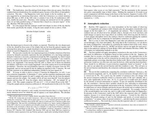
Absolute Ecliptic Latitude
mlim
00 ◦ -15 ◦ 4.71
15 ◦ -30 ◦ 4.65
30 ◦ -45 ◦ 4.46
45 ◦ -90 ◦ 4.42
Here the deepest part is closest to the ecliptic, as expected. Therefore, the very deepest part
of the sky should be those areas of the ecliptic that are far from the galactic equator, and
choosing those areas for our sample should give us the deepest possible limiting magnitude,
which we need for Hipparchos to see the Commentary stars.
C12 We must also consider the very important question of whether a function of the form
chosen by Schaefer accurately represents the true probabilities of a star being cataloged.
Schaefer’s function is inversely symmetrical around the 50% magnitude, by which I mean
that for a typical mlim value of 5, the chances of cataloging a magnitude 7 star would be
exactly the same as the chances of missing a magnitude 3 star. But this cannot be true, since
there is one magnitude 3 star missing from the ASC (η Tauri) out of about two hundred
possibilites, while there is not a single magnitude 7 star in the catalog out of several thousand
possibilities. Therefore, the real probability function is slightly assymetric from the 50%
magnitude, and we can account for this by adding an exponent to the P function. We will
find this exponent as an additional independent variable in our least squares fit.
C13 To recap, in order to derive a correct P function for Hipparchos, we will: 1) use
post-extinction magnitudes; 2) determine F , mlim, and the exponent simultaneously using
a 3-dimensional least-squares fit; and 3) sample only areas of the sky far from the galactic
equator and near the ecliptic. Our sample will be all stars more than 60 ◦ from the galactic
equator and less than 30 ◦ from the ecliptic, above declination −30 ◦ , for latitude 36 ◦ at
epoch −140. This sample comprises 355 stars of V < 6.9, of which 58 are in the ASC. 12
Using this sample and an extinction coefficient of .182 (justification for this in fn 18), I find:
P = 1/(1 + e 1.69(µ−6.53) ) 10 (2)
It turns out that the exponent is only weakly recovered because there is a large family of
nearly identical curves for which the sum of squares is not much different. The absolute
11 This will also allow us to use a slightly thicker atmosphere than otherwise.
12 Of the 355, twenty-nine are in the Commentary. But as we have seen above in fn 9, our task of
making the Commentary visible will be much easier if we use a P function derived from the ASC.
Some may object that, if Ptolemy observed the ASC, then we would expect his P function to differ from
that of Hipparchos. But since the overwhelming weight of evidence (e.g. figure 1) points to Hipparchos
as the ASC’s observer, we are entitled to provisionally assume this as being true. If, as Schaefer asserts,
the debate on the astrometric evidence has come to a standstill, it is only because Ptolemy’s defenders
have completely surrendered on that front. The resoundingly conclusive astrometric evidences of
Newton 1977, Rawlins 1982, Graßhoff 1990, Rawlins 1994, and now Duke 2002 have inspired no
worthwhile counter-arguments from any Ptolemy apologist, significantly including Schaefer himself.
Pickering Hipparchos StarCat South Limits 2002 Sept DIO 12 ‡1 11
least-squares value occurs at very high exponents, 13 but the uncertainty in the exponent
also grows unacceptably large at these values. Holding the exponent to 10 results in an
easier computation with little change in the fitness of the function. Equation 2 yields a 50%
probability of observation at µ = 4.97, nearly the value we would have gotten without the
exponent (µ = 4.93).
D
Atmospheric extinction
D1 Rawlins 1982 supposed a very clear atmosphere on the best nights of observing
(k = .15 magnitudes per airmass) while Schaefer puts the atmosphere considerably more
opaque on the best nights (k = .23 magnitudes per airmass). This is important, since
southern stars are all observed at low altitudes (that is, through a lot of air and dust), and
small changes in opacity have large effects on visibility when observing near the horizon.
A more opaque atmosphere moves the catalog’s observer southward (putting the southern
stars higher in the sky to compensate for atmospheric extinction; see §H5.)
D2 But it is easy to show that Hipparchos (and other pre-industrial astronomers) observed
through a very clear atmosphere. By using data in the Commentary, we can derive
the clarity of Hipparchos’ atmosphere by examining the southern limit of this work, whose
latitude (36 ◦ North) and epoch (ca. 140 BC) are known; and we can apply the same procedures
to the naked-eye catalogs of Tycho Brahe (1601) and Johannes Hevelius (1660). We
will employ two independent methods to do this.
D3 Our first method will apply atmospheric extinction to the stars in the Commentary,
and check for differences in brightness based on their position in the sky. Suppose, for
example, that we assume a too-thick atmosphere. In that case, the cataloged stars in the
very southern part of the sky will be extincted far too much; they will have post-extinction
magnitudes greater, on average, than than those farther north. But it is silly to expect that an
astronomer would see very dim stars only near the horizon, while ignoring them elsewhere.
There should be no difference in post-extinction magnitudes based on location 14 in the
sky, and we can adjust the aerosol fraction until this condition is met. This will give us
the aerosol fraction (and therefore, the extinction coefficient) under which the catalog was
observed.
D4 We test for this condition by computing the correlation coefficient r between µ, the
post-extinction magnitude, and X a, the number of aerosol airmasses through which a star
is viewed (see fn 39). For a given star, the number of airmasses does not change with
the aerosol extinction coefficient (which is a function solely of the star’s altitude), but µ
does, quite significantly for low stars. So X a is a good way to weight each star’s datum
by the amount of aerosol information it contains. If stars are randomly distributed in the
sky, the correlation r between these variables should be zero, indicating no relationship
between post-extinction magnitude and position in the sky. In practice, however, there may
be slight biases at various latitudes and epochs because the actual stars at southern limit for
a given observer may be distributed non-randomly in magnitude. For example, Canopus
is the second-brightest star in the sky, and it is right at the southern limit for Hipparchos.
Its presence in the Commentary (and in the ASC) drives the expected value of r slightly
negative, because it is viewed through very many airmasses. I tested for this effect by
creating 100 pseudo-catalogs of stars for the latitudes and epochs of several naked-eye
astronomers, 15 at various values of aerosol extintion k a, and deriving the mean correlation
coefficient for each k a. The result (fig 2) shows that the expected value of r is indeed close
13 This formally confirms that the P function is inversely assymetrical, since only an exponent of 1
results in a symmetric function.
14 This test was first suggested in Rawlins 1993 (DIO 3 §L10).
15 I confined these catalogs to apparent altitudes < 30 degrees, because seelction of stars higher than
that is not due to atmospheric effects.