Xenogen IVIS-200 user manual

© 2002-2006 Xenogen Corporation. All rights reserved.PN40156 Rev AXenogen Corporation860 Atlantic AvenueAlameda, California 94501, USAPhone: 510.291.6100Fax: 510.291.6196www.xenogen.comXenogen Technical Support1.888.810.8055 (US only)1.510.291.6275 (International)E-mail: ivistechsupport@xenogen.comDiscovery in the Living Organism, IVIS Imaging System and Living Image and either registered trademarks ortrademarks of Xenogen Corporation. The names of companies and products mentioned herein may be thetrademarks of their respective owners. Apple, Macintosh and QuickTime are registered trademarks of AppleComputer, Inc. Microsoft, PowerPoint and windows are either registered trademarks or trademarks of MicrosoftCorporation in the United States and/or other countries. Adobe and Illustrator are either registered trademarks ortrademarks of Adobe Systems Incorporated in the United States and/or other countries.

Contents9 Measurements, Units, and Calibrations . . . . . . . . . . . . . . . . . . . . 799.1 Regions of Interest (ROI) . . . . . . . . . . . . . . . . . . . . . . . . . . . . . . . . 809.2 Units . . . . . . . . . . . . . . . . . . . . . . . . . . . . . . . . . . . . . . . . . . . 839.3 Flat Fielding . . . . . . . . . . . . . . . . . . . . . . . . . . . . . . . . . . . . . . . 859.4 Cosmic Ray Corrections . . . . . . . . . . . . . . . . . . . . . . . . . . . . . . . . . 8610 Auto ROIs . . . . . . . . . . . . . . . . . . . . . . . . . . . . . . . . . . 8710.1 Measurement ROIs . . . . . . . . . . . . . . . . . . . . . . . . . . . . . . . . . . . 8710.2 Subject ROIs . . . . . . . . . . . . . . . . . . . . . . . . . . . . . . . . . . . . . . 9011 Background Sources . . . . . . . . . . . . . . . . . . . . . . . . . . . . . . . 9311.1 Electronic Background . . . . . . . . . . . . . . . . . . . . . . . . . . . . . . . . . 9311.2 Background Light On the Sample . . . . . . . . . . . . . . . . . . . . . . . . . . . 9411.3 Background Light From the Sample . . . . . . . . . . . . . . . . . . . . . . . . . . 9612 Dark Charge Management . . . . . . . . . . . . . . . . . . . . . . . . . . . . 9912.1 Dark Charge Measurement . . . . . . . . . . . . . . . . . . . . . . . . . . . . . . . 9912.2 Dark Charge Subtraction . . . . . . . . . . . . . . . . . . . . . . . . . . . . . . . 10012.3 Read Bias and Drift . . . . . . . . . . . . . . . . . . . . . . . . . . . . . . . . . 10112.4 Automatic Background Measurements . . . . . . . . . . . . . . . . . . . . . . . 10113 Data Management . . . . . . . . . . . . . . . . . . . . . . . . . . . . . . . . . 10313.1 Storing Living Image ® Data . . . . . . . . . . . . . . . . . . . . . . . . . . . . . 10313.2 Retrieving Living Image Data . . . . . . . . . . . . . . . . . . . . . . . . . . . . 10413.3 Importing Data into Living Image Software . . . . . . . . . . . . . . . . . . . . . 10614 Fluorescent Imaging . . . . . . . . . . . . . . . . . . . . . . . . . . . . . . . 10714.1 Description and Theory of Operation . . . . . . . . . . . . . . . . . . . . . . . . 10714.2 Understanding Filter Spectra . . . . . . . . . . . . . . . . . . . . . . . . . . . . . 11014.3 Acquiring Fluorescent Images . . . . . . . . . . . . . . . . . . . . . . . . . . . . 11214.4 Image Units . . . . . . . . . . . . . . . . . . . . . . . . . . . . . . . . . . . . . 11414.5 Working with Fluorescent Samples . . . . . . . . . . . . . . . . . . . . . . . . . 11415 Spectral Imaging (IVIS ® Imaging System 200 & 3D Series) . . . . . . . . . 12715.1 Spectral Imaging Procedure . . . . . . . . . . . . . . . . . . . . . . . . . . . . . 12715.2 Spectral Imaging Theory . . . . . . . . . . . . . . . . . . . . . . . . . . . . . . . 13016 Structured Light (IVIS ® Imaging System 200 & 3D Series Only) . . . . . . 13916.1 Theory of Operation . . . . . . . . . . . . . . . . . . . . . . . . . . . . . . . . . 139ii

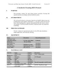
1. WelcomeCCD cameraImaging chamberAcquisition computer and monitorFigure 1.1 IVIS ® Imaging System 50 SeriesCCD cameraImaging chamberAcquisition computer and monitorFigure 1.2 IVIS Lumina2

Living Image ® Software ManualCCDCameraCryogenic refrigeration unit& camera controllerImagingchamberAcquisition computer & monitorFigure 1.3 IVIS ® Imaging System 100 SeriesCCDcameraOptional XGI-8 GasAnesthesia SystemMonitorAcquisitioncomputerFigure 1.4 IVIS Imaging System 200 Series3

1. WelcomeImaging chamberCCDcameraOptional XGI-8 GasAnesthesia SystemMonitorThermoCubewater chillerCamerapowersupplyAcquisitioncomputerFigure 1.5 IVIS ® Imaging System 3D SeriesThe system takes very low-light level images, stores them, and displaysthem for subsequent analysis. This manual describes the use of the IVISImaging System and Living Image software for a typical in vivoimaging application. Some aspects of general purpose, low light-levelimaging such as sensitivity and binning, measurements andcalibrations, background sources of light, and dark charge managementare also discussed.1.2 Living Image ® SoftwareThe software is developed within a powerful data analysis andprogramming environment called WaveMetrics IGOR Pro 1 . TheLiving Image software creates a custom environment that is used forboth data acquisition and analysis as described in this manual. LivingImage software and Igor Pro run on both Macintosh ® and Windows ®computers. To start Living Image software under Windows, look forthe Living Image software icon in the Start-Programs-Living Imagemenu or on the desktop. For Macintosh computers, look for an alias inthe Apple ® menu or on the desktop.An overview of the Living Image software interface is shown in Figure1.6. The standard panels include an image acquisition control panel,image display and analysis window, system status and dialog window,and a lab book window. Located in the top menu bar are tools for bothIGOR Pro and Living Image software. Menu items that apply to Igor1. WaveMetrics, Inc. retains copyright of Igor Pro 1992-20044

Living Image ® Software ManualPro only, and are not supported by Living Image software, remaininactive (disabled), helping to avoid interface clutter and confusion.See Chapter 6, page 43, for information on enabling these features. Referto the Igor Pro manual (available in the Help menu) for information oncommands not supported by Living Image software.Figure 1.6 Living Image ® software user interfaceSections of the Living Image manual may be viewed by selectingLiving Image-Living Image Help. A PDF format version of themanual is also available in Start-Programs-Living Image (Windows)and in the Help menu (Mac). Help for specific controls can also beviewed as shown below.OperatingSystemProcedure for Viewing HelpWindowsMacintosh OSXHold the cursor over the item of interest and look for the helpmessage in the system status line.Same as above but the user must first activate Show IGORTips from the top level Help menu.This Living Image software manual is organized according to thepanels and menu items shown in (Figure 1.6). Commands and controlsassociated with the system control panel, the image display andanalysis window, and the main menu bar items are described in separatesections. Later sections provide more details on a number of topicsrelated to in vivo imaging.The nomenclature in this manual uses bold text to indicate buttons,checkboxes, and menu items, e.g. Help. Bold text separated by hyphens5

1. Welcomeis used to indicate pull-down menus, e.g., Living Image Tools-ShowCursors. Names of windows and panels are capitalized but not bold,e.g., Measurements Table.1.3 Xenogen Technical SupportTechnical Support: 1.888.810.8055 (US)1.510.291.6275 (International)Main Telephone: 1.510.291.6100E-mail:IVISTechSupport@xenogen.comFax: 1.510.291.6196Address:Xenogen Corporation860 Atlantic AvenueAlameda, CA 945016

Living Image ® Software Manual2Quick Start Guide to Acquiring ImagesThis section consists of a "Quick Start" procedure to acquire anilluminated image of a sample (photographic image) followed by a nonilluminatedimage of light emission from the sample (luminescentimage). No analysis is described. This procedure is intended as a briefguide that can be followed step by step. For more detailed information,see the sections that immediately follow. This procedure assumes thatthe system power is on. If power to the system is not on, see the IVIS ®Imaging System Hardware Manual.1. If it is not already on, start up the acquisition computer and start theLiving Image ® 2.6 software program from the Windows StartMenu. Log in by selecting your initials from the drop down menu,or if you are a new user, enter your initials and click DONE. Asystem control panel will appear in the lower right corner of themonitor (Figure 2.1).Figure 2.1 IVIS System Control Panel.2. Click the Initialize IVIS system button in the camera controlpanel. After initialization, the Temperature Status box in the7

2. Quick Start Guide to Acquiring Imagescenter of the panel should be green, indicating that the CCD camerais adequately cooled. (If you are using the IVIS ® Imaging System50 Series or the IVIS Lumina, allow 10 to 15 minutes for thecamera to reach the proper temperature.) The Temperature Statusbox changes from red to green when the CCD camera has reachedthe proper operating temperature.3. Place the sample to be imaged in the center of the stage in theimaging chamber. Close the door.4. Select the desired Field of View from the pull down menu on theleft side of the control panel.5. Enter the approximate (1 cm) Subject Height in the lower leftentry box.6. Click the Acquire continuous photos button to check the subjectposition. (This step is optional.) Close this window and repositionthe subject if necessary.7. Check the Overlay box in the control panel and set the ExposureTime, binning, and f/stop for the luminescent image. If unsure ofwhat exposure time to use, it is best to start with low sensitivitysettings (10 sec, Medium, f/1) and increase as necessary.8. Click the Acquire button on the control panel.NOTEDuring the luminescent image acquisition, the Acquire buttonbecomes a Stop button, which can be used to terminate theexposure, if desired.9. After the exposure is complete, the overlaid image is displayed.Edit the information in the Change Information window and clickDone. Always click Done in the Image Information window beforeproceeding.10. Confirm that the signal of interest is above the noise level(recommend >600 counts) and below CCD saturation (~60,000counts). If the signal level is unacceptable, adjust Exposure Timeor Binning and repeat the image acquisition.11. Upon acquisition, an image is not automatically saved, but it isautomatically named using the operators initials, and a date andtime stamp. To save the image, choose Save Living Image Data(under the Living Image menu item), select the Format "Save allLiving Image Data Files", check the box "Save Lab Book", thenclick Save.This completes the data acquisition. If desirable, adjust the display withthe Max Bar or Min Bar slider. To obtain additional images, beginwith Step 3 above.Subsequent analysis is described in Chapter 4, page 21, and can beconducted immediately or deferred until later, after additional imagesof the sample have been acquired.8

Living Image ® Software Manual3 Control Panel for IVIS® Imaging SystemsBasic Controls . . . . . . . . . . . . . . . . . . . . . . . . . . . . 9Fluorescence Option . . . . . . . . . . . . . . . . . . . . . . . 16IVIS Imaging System 200 Series Options . . . . . . . . . . . . 17IVIS Imaging System 3D Series Options . . . . . . . . . . . . 183.1 Basic ControlsTypically, image acquisition on all IVIS Imaging Systems involvesplacing a sample on the stage, adjusting camera settings such as fieldof-view(FOV), sample height, and exposure time, binning, andacquiring the image. Most sample images are actually a composite oftwo images. The first image is a short exposure of the sampleilluminated by lights located in the top of the imaging chamber. SeeFigure 3.1. This image is referred to as a "photographic image" and isdisplayed as a grayscale (black and white) image. The second image isa more sensitive exposure of the sample taken in darkness to recordlow-level luminescent emissions. This portion of the image is referredto as the "luminescent image". The luminescent information, displayedin pseudo-color representing intensity, is overlaid on top of thephotographic image to form an "Overlay Image" to create what'sreferred to as an "Overlay image". See Figure 3.2. The acquisition andoverlay of the two images is done automatically by Living Imagesoftware. For IVIS Imaging Systems with fluorescent imagingcapabilities, a fluorescent image may be acquired and displayed in thesame manner as the luminescent image. See Section 3.2, page 16.IlluminationLEDsOpening forcamera lensSample stageFigure 3.1 IVIS ® Imaging System 100 Series, interior view.9

3. Control Panel for IVIS ® Imaging SystemsFigure 3.2 Example image overlay: luminescent pseudocolor image ongrayscale photographic image.The IVIS System Control panel controls acquisition functions for allIVIS Imaging Systems. See Figure 3.3. Optional controls for the IVISImaging System 200 Series and systems with fluorescence capabilitieswill be discussed later in this section. Each control contains a built-inhelp message that can be displayed by moving the cursor over thecontrol. The help message will appear in the system status line(typically located in the lower left corner of the screen on an IVISImaging System acquisition computer). A detailed description of eachcontrol is given below. The commands are listed in the general order inwhich they should be used when acquiring an image. See Chapter 2,page 7 for step-by-step procedures.Figure 3.3 IVIS System Control Panel for camera system setup and imageacquisition.Initialize IVIS System initializes the IVIS Imaging System. It must beused each time Living Image software is started or if the power has beencycled on either the camera controller or the imaging chamber. It canalso be used to reset to startup conditions, which is sometimes useful inerror situations. The initializing procedure moves every motor-drivencomponent (stage, lens, etc.) in the system to a "home" position, resets10

Living Image ® Software Manualall electronics and controllers, and restores all software variables todefault settings.System Status is the region of the camera control panel that displaysCCD temperature information and status messages describing currentoperation of the system. The temperature settings should be checkedafter initialization. The top line, labeled Temperature, monitors thecurrent temperature of the CCD. If the measured CCD temperature iswithin the acceptable range, a green box is displayed. If the temperatureis out of range, a red box is displayed; and if the system has not beeninitialized, a blank box is displayed. Click once on the colored box toview the actual temperature. Current and demand temperatures will bevisible for five seconds. The CCD demand temperature is fixed andshould not be changed by the user. Electronic feedback controlmaintains the CCD temperature to within a few degrees of the demandtemperature. If the temperature status control box is green, thisindicates that it is "locked," and the IVIS is ready for imaging. If thestatus box indicates "unlocked" for a long period, contact IVISTechnical Support.On the IVIS Imaging System 200 Series, the sample stage temperatureis also displayed and controlled from the System Status panel. Thesample stage temperature is set to 37° C by default, but may be changedby the user to any temperature within the range of 25°- 40° C.Field of View (FOV) sets the size of the imaging region on the samplestage by adjusting the height of the sample stage and adjusting theposition of the lens. The FOV is the width, in centimeters, of the squarearea on the stage that is to be imaged. Standard calibrated FOVpositions are indicated by A, B, C, D, E, and correspond approximatelyto the widths shown in the table below.Imaging SystemIVIS ® Imaging System 50Series and IVIS LuminaIVIS Imaging System 100SeriesIVIS Imaging System 200SeriesFOV values for positions A, B, C, and Drespectively (and E for IVIS 200)5, 7.5, 10 or 12.5 cm10, 15, 20, or 25 cm4, 6.5, 13, 20, 25 cmIn addition to selecting the viewing area, the FOV control indirectlyaffects the depth-of-field. The depth-of-field refers to the range overwhich the image is in focus. The depth-of-field is affected by both theFOV and the f-stop (see f-stop discussion below). Similar to amicroscope, the depth-of-field decreases as the magnificationincreases. A smaller FOV (higher magnification) will have a narrowerdepth-of-field.Focus and Subject Height is a group of controls that sets the focalplane at a particular location above the stage. Focusing is done by oneof two methods (a third method is available with the IVIS ImagingSystem 200 Series). One method is to enter the estimated height of thesubject, in centimeters (accuracy of 0.5 cm is usually adequate), in theSubject Height box. This adjusts the stage position so that the focalplane of the lens/CCD system is positioned at the estimated height11

3. Control Panel for IVIS ® Imaging Systemsabove the stage. The estimated height does not have to be the maximumheight of the subject. For example, if the goal is to monitor luciferaseexpression in the joint of a mouse leg, then the subject height should bethe height of the leg above the platform, typically a few millimeters.However, if the user is interested in imaging a tumor on the uppermostdorsal side of a mouse, the full height of the animal (about 1.5-2.0 cm)should be used. The default setting at startup for subject height is 1.5cm.In addition to getting a sharp image, there are safety implicationsrelated to the subject height, particularly on IVIS Imaging System 200Series. Placing a large subject, e.g., 10 cm high, on the stage andentering a height of zero and choosing a small FOV will result in thestage being positioned such that the subject may make contact with thetop of the imaging chamber. Although built-in protections preventdamage to the instrument, users should always pay close attention to thesubject height.A second method for focusing, called Manual focus, is available in thepull down menu. In this method, a photographic image is acquired anddisplayed in the Manual Focus Control panel, using the f/stop settingspecified for the Luminescent image. See Figure 3.4. The Up and Downbuttons refer to the incremental movement of the stage, while Fine,Normal, and Coarse refer to the size of the increment. Clicking the Upand Down buttons changes the focus. When optimum focus isachieved, close the panel. The resulting focal plane height will beentered automatically into the Subject Height box.Figure 3.4 Manual Focus Control Panel. Illustration of manual focusing at f/1.Use the Up and Down controls to fine tune the focus position.Imaging Mode presents three checkboxes that are used to selectbetween the photographic and luminescent (or fluorescent) imagingmodes described above. The default is Overlay, which automaticallytakes a photographic image followed by a luminescent image, thenoverlays them. Overlay is the mode recommended for most imagingapplications.Exposure Time controls the length of time that the shutter is open forphotographic and luminescent images. In the photographic settings,when "Auto" is checked, the exposure time will automatically be12

Living Image ® Software Manualadjusted to produce a good photograph. Luminescent images typicallyhave longer exposure times that need to be adjusted, depending on thebrightness of the subject. The luminescent or fluorescent signal level isdirectly proportional to exposure time. Luminescent exposure time ismeasured in units of seconds or minutes. The minimum calibratedexposure time is 0.5 seconds. There is no limit on the maximumexposure time, but usually there is little benefit to exceeding 5 minutesfor animal imaging. The goal is to adjust the exposure time to producea signal that is well above the noise (recommend >600 counts) but lessthan the CCD camera saturation of ~60,000 counts.Binning increases the pixel size on the CCD, which delivers highersensitivity at the expense of spatial resolution. The high resolutionCCDs used in IVIS Imaging Systems contain between 1024x1024 and2048x2048 elements. Depending on the subject being imaged, thisresolution is usually much higher than necessary. The CCD hardwarecan be binned so that NxN areas of the CCD are summed beforereadout, where N is the binning level. This concept is illustrated inFigure 3.5. Binning a luminescent image results in a significantimprovement in the signal-to-noise ratio. Although spatial resolution isdegraded at high binning (pixels become large), this is often acceptablefor in vivo images where light emission is rather diffuse. Binning pulldownmenu choices for luminescent images are small, medium, andlarge, with the default set to medium. Each change in binning changesthe sensitivity by a factor of four. For example, Medium binning is fourtimes more sensitive than small binning. The user can opt to see theactual binning numbers by selecting the Living Image Tools-Preferences option from the pull-down menu and using the CameraSettings button to select Manual Binning Values. Recommendedbinning numbers for luminescent images are 1-4 for high-resolutionimaging of cells or tissue sections, 4-8 for standard in vivo images, and8-16 for very dim in vivo images requiring the highest sensitivity. SeeChapter 8, page 73.Binning = 1 Binning = 2 Binning = 4CCD pixelSignal 4 times larger.Spatial size double.Figure 3.5 A small segment of the CCD at binning = 1, binning = 2 (4 pixelsummed together), and binning = 4 (16 pixels together)f/stop controls the aperture of the lens on the camera. A larger numberindicates a smaller aperture setting and lower sensitivity. The smallestf/stop on all IVIS Imaging Systems is f/1, which corresponds to thewidest lens opening and the most sensitive setting. The detected signalscales inversely with the square of the f-number. The aperture size, or13

3. Control Panel for IVIS ® Imaging Systemsf/stop, controls both the amount of light detected and the depth-of-field.See Fig. 3.6. A smaller aperture results in reduced sensitivity butimproved depth of field, which produces a sharper image of an objectwith varying height. Typically, the photographic image is taken with asmall aperture (f/8 or f/16) to give the sharpest image. The luminescentimage is taken with a large aperture (f/1) to maximize sensitivity. All f/stop values are calibrated and the user is free to change these settings.For cases in which spatial resolution is known to be important, the usershould select the Focus-manual option to see how sharp the image willbe at the selected f/stop. This is especially important at the highmagnification settings available on the IVIS Imaging System 200Series because the depth of field is very narrow, on the order of 1-3 mm.Figure 3.6 f/stop. Left: lens wide open at f/1; right: lens closed down at f/8.Emission Filter controls the filter wheel in front of the CCD lens. Thiswheel may have different types of filters installed for eitherfluorescence or spectral imaging applications. The number of filterslots ranges from 6 - 24, depending on the system. The desired filter ischosen from the pull down menu. For bioluminescent imaging, thefilter wheel is typically set to "Open," which is a position with no filter.Acquire initiates the image acquisition using the conditions chosen bythe photographic and/or luminescent controls prior to the start ofacquisition. During image acquisition, the Acquire button becomes aStop button that can be used to terminate the exposure. At the end ofacquisition, a Change Info panel is presented. This panel allows theuser to enter descriptive information about the image. The descriptorsappear as labels in the image window and can be used to help identifythe image data later. Always click Done on the Change Info panelbefore proceeding, even if you don't wish to label the image. SeeChapter 13, page 103.Acquire Continuous Photos sets the camera in "live" photographicimaging mode. In this mode, a series of illuminated photographicimages (frames) are taken rapidly and displayed sequentially to give avideo-like effect that is useful for checking subject position and14

Living Image ® Software Manualwatching for animal movement. The exposure time per frame, f/stop,and filter setting used in this mode are the same as those set forphotographic mode. The system will take ten photos, thenautomatically stop in order to lengthen the service life of the shutter.Lights On manually turns the illumination lights in the top of theimaging chamber on and off for inspection. This is not needed forimaging, since the lights turn on and off automatically.Figure 3.7 Sequential Imaging Panel used to define a sequence of images for acquisition.Select Sequential Mode opens up a new panel that allows the user todefine an entire sequence of images to be taken with a single click ofthe Acquire Sequence button. See Figure 3.7. This option can be usedto take a kinetic series of images (a sequence in time), a sequence ofimages with different filters, or a sequence varying any other parameteravailable in the IVIS System Control panel. Select the camera settingsfor the first image using the IVIS System Control panel. Then click theSet button in the Sequential Setup panel. This will load the parametersinto the Sequential Setup table. Enter a delay time if desired, which isthe time from the start of one image to the next, change the acquisitionparameters if desired, then click Set again to load the next image. If the15

3. Control Panel for IVIS ® Imaging SystemsDelay Time is set to a number smaller than the acquisition time (forexample, 0.1 minutes), then the acquisition of the subsequent imagewill start immediately. Up to 99 entries can be made in the sequencetable. The Clear One and Clear All buttons allow the user to clear asingle entry or all entries from the table, respectively. The Save andRecall buttons allow the user to save the setup on disk and recall it later.To edit an existing Sequence, click Edit Sequence, highlight thesequence number you want to edit, change the acquisition settings tothe new parameters, then click Change. When finished editing, clickDone. After setup of the sequential table has been completed, clickAcquire Sequence to start the sequence. Thumbnail views of theimages will appear as the image acquisition proceeds. To return tosingle-image acquisition, click on the Select non-sequential modebutton. See Chapter 5, page 39 for more information on analysis anddisplay of sequences.3.2 Fluorescence OptionFor IVIS Imaging Systems configured with the fluorescence option,there are additional controls that appear in the IVIS System Controlpanel. See Figure 3.8. For more details on fluorescent imaging andoperation of the fluorescence acquisition controls, see Chapter 14,page 107.Figure 3.8 IVIS System Control panel for fluorescence imaging.The Excitation Filter allows the user to select from up to 11fluorescence excitation filters (plus one blocked position) from thepull-down menu. By default, the filter is set to “Block” forbioluminescent images. It is important to always match filters (GFPexcitation with GFP emission), as a mismatch, e.g., GFP excitationwith Open emission, may result in an image that is over-exposed orsaturated.Filter Lock locks the excitation and emission filters together (forexample, GFP excitation with GFP emission) to avoid mismatchedfilters and the possibility of over-exposed images. This option shouldbe checked during normal fluorescence imaging.16

Living Image ® Software ManualFluor Lamp Level allows the user to set the fluorescence lampemission level to Off, Low, High, or Inspect. Low emission isapproximately 18% of High. It is recommended to always use High ifpossible. If a fluorescent image is too bright, then use other controlssuch as f/stop, Binning, or Exposure Time to reduce the signal.NOTEThe f/stop setting defaults to f/2 for fluorescence imaging. While thisis the recommended starting point, the f/stop may be adjusted ifnecessary.Inspect turns the fluorescent lamp on manually, allowing the user toinspect the illumination inside the IVIS Imaging chamber. Beforeselecting Inspect, verify that the emission and excitation filters areselected as desired. When Inspect is selected, the software will firstmove the excitation and emission filters to the positions currently set inthe respective drop-down menus before turning on the fluorescentlamp. This control is only used for inspection. The software controlson/off cycling of the lamp automatically during imaging and will returnthe Fluor Lamp Level to its previous High or Low setting for imaging.3.3 IVIS Imaging System 200 Series OptionsIn addition to the fluorescence control panel settings described above,the IVIS Imaging System 200 Series offers control options relating tothe scanning galvanometer. These options are shown in Figure 3.9 anddescribed below.Figure 3.9 IVIS Imaging System 200 Series Control Panel.Enable Alignment Grid activates a laser-generated alignment gridinside the IVIS System 200 Series imaging chamber when the door isopened. The alignment grid is set to the size of the FOV selected in theField of View pull-down menu. The grid will turn off automaticallyafter 2 minutes to avoid excessive wear on the laser. If alignment of thesubject is not complete after 2 minutes, check the Enable alignment17

3. Control Panel for IVIS ® Imaging Systemsgrid box again to turn on the grid. The horizontal cross hair on thealignment grid is offset appropriately to take into account the height ofthe object entered in the Subject Height box.Focus-Scan Mid Image is another option for determining subjectheight and is selected from the Focus drop down list. When this optionis selected, the laser beam is scanned horizontally across the middle ofthe image to determine the maximum subject height along this line.This option works reasonably well for animal imaging because the peakheight is clearly identified as the maximum height on the dorsal sidealong the mid-plane of the animal. This method of focusing is notrecommended for objects with a great deal of structure such as wellplates, or for the high magnification (FOVA = 4.0 cm) field of view. Inthese or similar situations, Manual focus or Subject Size focusmethods are recommended.Structure enables the structured light system for determining surfacetopography. Selecting this option will acquire an image of parallel laserlines scanned across the subject. This is called the structured lightimage. From this image, the surface topography of the subject can bedetermined. This information serves as input for the DiffuseLuminescence Imaging Tomography (DLIT) code for reconstructingthe location and brightness of luminescent sources. When Structure isselected, the structured light image will be acquired automaticallyalong with the photographic and luminescent (if selected) images whenthe Acquire button is clicked. The f/stop is set to a default setting of f/8 and the exposure time is set to 0.2 seconds for the structured lightimage. The spatial resolution of the computed surface depends on theline spacing of the structured light lines. Line spacing and imagebinning are automatically set to the optimal values determined by thestage position (field of view) and cannot be changed by the user.3.4 IVIS Imaging System 3D Series OptionsThe IVIS Imaging System 3D Series offers control options relating tothe position of the CCD camera during image acquisition. Theseoptions are shown in Figure 3.10.18

Living Image ® Software ManualSequentialSetup windowIVIS System Control panelFigure 3.10 IVIS Imaging System 3D Series Control PanelAngle indicates the starting position of the CCD camera relative to theimaging platform. The first image in a sequence is acquired at thisangle.Inc is the number of degrees between each successive position of theCCD camera during the acquisition of an image sequence.Structure enables the structured light system for determining surfacetopography (for more details see page 18).NOTEThere is no FOV option for the IVIS Imaging System 3D Series sinceimages are acquired at the same FOV, but at different angles.19

3. Control Panel for IVIS ® Imaging Systems[This page intentionally left blank.]20

4Living Image ® Software ManualImage Display and Analysis WindowImage Display Tools . . . . . . . . . . . . . . . . . . . . . . . 22Region of Interest Tools . . . . . . . . . . . . . . . . . . . . . 22Physical Units . . . . . . . . . . . . . . . . . . . . . . . . . . . 26Display Mode . . . . . . . . . . . . . . . . . . . . . . . . . . . 27Image Correction Check Boxes . . . . . . . . . . . . . . . . . 31Print & Zoom . . . . . . . . . . . . . . . . . . . . . . . . . . . 32Image Window Contextual Menus . . . . . . . . . . . . . . . 34Figure 4.1 represents a typical image window display that appears whena Living Image data set is opened or acquired. The main part of thewindow is most often a pseudocolor image referred to as theluminescent or fluorescent image overlaid on a photographic image.Generally, anything that is described in this manual as being applicableto the luminescent image will also be applicable to fluorescent imagesunless otherwise noted. At the top of the image window are analysistools used for controlling the image display and taking measurements.Individual controls in the analysis panel are described below. On theright side of the image window is a color bar that shows the relationshipbetween the pseudocolors in the image and the numerical values of theimage data. At the bottom of the window display is a section thatcontains labeling information generated by both the user and theimaging system. This section describes use of the individual controlsfound in the image window.Figure 4.1 Living Image data set in the Image Window.21

4. Image Display and Analysis Window4.1 Image Display ToolsMax Bar sets the maximum value for the range of data associated withthe color bar for the image.Min Bar and Min Bar Slider sets the minimum value for the range ofdata associated with the color bar for the image. The minimum valuealso serves as a threshold below which data in luminescent orfluorescent images are not displayed. When creating overlays, thisallows the underlying photographic image to be viewed in regionswhere top-layer luminescent data is below the threshold.NOTEWhile Max Bar and Min Bar can dramatically affect the appearanceof the displayed image, the numerical values associated with theimage contents DO NOT change and the resulting measurement isindependent of display conditions. For more details on color bars andpseudocolor images, see Chapter 7, page 69.Log can be used to change the pseudocolor display from a linearrelationship between numerical data and displayed colors to alogarithmic relationship. In doing so, the range of the meaningfulnumerical data that can be displayed is significantly increased.Full sets the Max Bar and Min Bar values to correspond to themaximum and minimum data values in the image, respectively.Auto uses an algorithm to set Max Bar and Min Bar to levels thatprovide a visually pleasing display, while suppressing the backgroundnoise. However, the Auto settings may not always give desirableresults, in which case further adjustments can be made manually usingthe Max Bar and Min Bar controls.Bright adjusts the brightness of the photographic image.Gamma adjusts the "gamma" of the photographic image, which isrelated to image contrast. This often improves the quality ofphotographic images, particularly for dark samples.4.2 Region of Interest ToolsCreate may be used to create one or more new Regions of Interest(ROIs), which are measurement tools used to quantify the amount oflight emission in specific areas of the image. If the Apply to Sequencecheck box is present, new ROIs are created in all the images within thesequence. See Chapter 5, page 39. An example of a Circle ROI is shownin Figure 4.2. For more on measurements and ROIs, see Chapter 9,page 79.22

4. Image Display and Analysis WindowFigure 4.3 Pull-down list of available ROI types and two user-created customROIs.Settings is located to the right of the type pull-down and is onlydisplayed when Auto 1 or Auto All is selected in the Number pulldownmenu. See Figure 4.4. This button is displayed during autocreation of both Measurement ROIs and Subject ROIs. Selecting thisbutton opens up the settings panels described below. Also see Chapter10, page 87.Figure 4.4 Settings button for auto creation of a Measurement ROI or a SubjectROI.The Auto ROI Settings panel controls the auto ROI settings forMeasurement ROIs in the top image window. See Figure 4.5. The ROIEdge Value controls the fraction (displayed as a percent) of the peakvalue at which the ROI contour is drawn. If the Use Background Offsetcheck box is checked and an appropriate Background ROI is set to beused as background for future ROIs (see the ROI Properties Panel andContextual Menus) then the average background level in thebackground ROI will be removed before computing the ROI EdgeValue. A background offset is also used when this box is checked andthe new Measurement ROIs created are inside a Subject ROI that has aBackground ROI linked to it. The Lower Limit controls the minimumpeak height of an auto ROI created in an Auto All search. This limit isexpressed as a multiple of the image window Min Bar setting. MinROI size controls the minimum required ROI size (expressed in pixels)for auto creation of an ROI. Reset to Default Values restores the checkbox to "checked" and sets the three numerical values described aboveto the default values of 5, 2, and 20 respectively. Recall PreferredValues can be used to recall stored values for the three numericalcontrols previously saved using the Store as Preferred Values button.Once selected, these preferred values act as default values for all imagewindows. A set of values unique to each individual user can be stored.The user ID of the current user is displayed in these buttons. In Figure4.5, the user ID is MDC. The Create Auto ROIs button allows thecreation of auto ROIs in the top image window and is equivalent tocreating ROIs with the Create button in the image window. This button24

Living Image ® Software Manualallows faster testing of different Auto ROI settings. The Removeexisting Auto ROIs first check box controls whether existing ROIs inthe top image window are removed before the creation of new AutoROIs. This function is equivalent to the Remove button in the imagewindow and exists merely to allow faster testing. Done closes the AutoROI Settings panel. The selected settings are stored for later use withthe top image window.Figure 4.5 Auto ROI Settings for auto creation of Measurement ROIs.The Auto Subject ROI Settings panel controls the settings for drawingSubject ROIs in the top image window. See Figure 4.6. Subject ROIsboxes are used to enclose a particular subject, usually a single animal.Auto creation of Subject ROIs will attempt to locate individual animalsin the photographic image and enclose each one with a Subject ROI.The default settings in this panel are optimized to locate animals,particularly light-colored mice on a dark background, but may also givegood results with other types of subjects. Cut-off parameter controlsa numerical value that may be used to "trim" distant parts of the animal,such as the tail, from the desired Subject ROI. The smaller the value,the larger the trim. Scale Factor is a multiplier applied to the size of theSubject ROI prior to display. A larger Scale Factor value may be usedto offset the effect smaller values of the Cut-off parameter have on aSubject ROI. Small ROI Limit A sets a lower limit for the smallestSubject ROI created. This limit is expressed as a percentage of thelargest Subject ROI to be created. By default, no Subject ROI will becreated if it is smaller than 10% of the size of the largest Subject ROI.Small ROI Limit B sets a second lower limit relative to the size of thetotal image area. Both of these limits are useful in preventing thecreation of Subject ROIs around very small parts of an image, such asreflections or dust. The Thresholding Method may be used to selectone of several algorithms designed to locate the edge of individualanimals within the image. The default is a Bimodal Method that workswell for light colored animals on a dark background, but if problems areencountered the user can try other algorithms for, possibly, betterresults. Other controls, including Reset to Default Values, RecallPreferred Values, Store as Preferred Values, Create Auto ROIs,25

4. Image Display and Analysis WindowRemove existing Auto ROIs, and Done–function as described abovein the Auto ROI Settings panel.Figure 4.6 Auto Subject ROI Settings for auto creation of subject ROIs.Measure initiates a measurement of any or all of the ROIs present inthe Image Window. Measurement results appear in both the Lab Bookand the Measurements Table. See "Lab Book,"page 58 and"Measurements Table," page 59. A brief summary of the measurementresults appears in the tools section of the image window above theimage display. The pull-down located directly below the Measurebutton controls which ROIs are to be measured. The default for allmeasures is All, however, individual ROIs may be selected. If theApply to Sequence check box is present, the specified measurementapplies to all images in the sequence. For more details, see Chapter 5,page 39.Remove may be used to remove the ROIs selected using the pull-downlocated directly below the Remove button.Apply To Sequence is present in all images that are part of a sequence.See Figure 4.7. If this box is checked, many of the image windowcontrols and their actions are set to modify all the images contained inthe sequence. See Chapter 5, page 39.Figure 4.7 Apply to Sequence option is available for images that are part of asequence.4.3 Physical UnitsThe Units pull-down menu is located immediately to the right of theRemove button. It can be seen in Figure 4.8, where it is set to Photons.This pull-down allows users to control absolute calibration of imagemeasurement data, one of the most powerful features of the LivingImage software and IVIS Imaging Systems. For more details, seeChapter 9, page 79. Individual settings for this control- Counts,Photons, Efficiency- are described below.26

Living Image ® Software ManualFigure 4.8 Units pull-down list set to photons.Counts allows the user to select the basic uncalibrated, raw data modeof image display. In this mode, image pixel contents are displayed asthe numerical output of the charge digitizer on the CCD. This numericaloutput is often referred to as counts, analog digitizer units (ADU), orrelative luminescence units (RLU). It is a number that is proportional tothe number of photons detected in the pixel. CCD digitizers on allmodels of IVIS Imaging Systems are 16-bit devices, which means thatthe number can vary from 0 to ~60,000. When a region of interest isintegrated, the units become photons/second and represent the numberof photons per second that radiate omnidirectionally from the regionspecified. The value displayed in an image may sometimes be slightlyoutside this range due to corrections made on the image data. SeeSection 4.5, page 31.Photons displays image data in terms of absolutely calibrated photonemission from the source. It is important to understand that while rawdata (Counts) is a measurement of photons reaching the CCD detector,the data displayed in Photons mode is calibrated for all instrumentsettings and parameters, and thus represents the actual physicalemission from the sample being imaged. Therefore, it is possible tocompare measurements made with different instrument settings (e.g.,differing exposure times, binning, FOV, etc.) as well as to comparemeasurements made on different instruments. In Photons mode, thequantity displayed is termed "radiance" and the units are photons/s/cm 2 /sr. In order for the displayed image to be calibrated, some of theimage corrections described in Section 4.5, page 31 must be applied.When Photons mode is selected, these corrections are applied and thecorresponding controls are deactivated. See Chapter 9, page 79.Efficiency is a choice present for fluorescent images only (availableonly on IVIS Imaging Systems equipped with fluorescent capabilities).If Efficiency is selected, the fluorescent emission image is normalized(divided) by a stored reference image of the excitation light intensity,which is measured for each excitation filter at every FOV and lamppower. These reference images are measured and stored in the LivingImage folder prior to instrument delivery. Normalizing fluorescentimages by the incident excitation intensity not only converts the displayto useful units, but also reduces the effect of spatial variations of theincident light. See Chapter 14, page 107.4.4 Display ModeThe Display Mode pull-down menu is located immediately to the rightof the Units pull down. It is used to control the type of image beingdisplayed. The choices are described below. See Chapter 7, page 69.27

4. Image Display and Analysis WindowFigure 4.9 DIsplay Mode set to Overlay.Photograph is a display mode that shows only an underlying grayscaleimage, which is captured when the IVIS imaging system illuminationlights are activated. See Figure 4.10.Figure 4.10 Image displayed in the Photographic display mode.Luminescent is a display mode that shows only the pseudocolorluminescent image obtained in an exposure with the IVIS ImagingSystem illumination lights deactivated. An example is show in Figure4.11. For image data taken in fluorescent mode on IVIS imagingsystems with fluorescent capability, the equivalent display mode istermed fluorescent, rather than luminescent. See Chapter 7, page 69.Figure 4.11 Section of an image window displayed in luminescent displaymode.Overlay is the default display mode where either a luminescent orfluorescent pseudocolor image is overlaid on a photographic image.See Figure 4.12. The lower limit of the pseudocolor image is controlledwith the Min Bar control, which sets a threshold below which data inthe luminescent or fluorescent image is not displayed. This allows theunderlying photographic image to be viewed in regions of the image28

Living Image ® Software Manualwhere the luminescent or fluorescent data is below the establishedthreshold.Figure 4.12 Section of an image window in Overlay display mode. The imagecomprises a luminescent image overlaid on a photographic image.Blend displays a blended image created from a combination ofphotographic and luminescent (or fluorescent) images where theluminescent image is partially transparent. When Blend is selected, aslider control appears and may be used to control the degree of opacityof the luminescent image. See Figure 4.13. A value of one is totallyopaque and is effectively an overlay. A value of zero is totallytransparent and is effectively a photographic image. This mode isuseful when you want to see the surface of the sample underlying thepseudo color.Figure 4.13 Blend slider controls the opacity of a blended image.29

4. Image Display and Analysis WindowFigure 4.14 Section of an image window in Blend display mode. The imagecomprises a luminescent image overlaid on a photographic image.Dark Charge displays the dark charge image stored in the image dataset. When viewing this image, it should be understood that dark chargeimages are multiplied by a factor (typically 10) that is stored along withthe image data. Hence, the displayed numerical values are notnecessarily the values being subtracted from the image data. SeeChapter 12, page 99.Saturation Map displays the region of the image, if any, for whichphoton emission is too intense to be quantitatively recorded whendetected by the CCD camera. ROI measurements should not be madeon these parts of the image. Measurements in other parts of the imagenot containing the saturated pixels will still be accurate (unless theimage is badly saturated).Figure 4.15 Section of an image window in Saturation display mode. Redareas represent saturated pixels.Fluorescent Bkg displays the instrument fluorescence background(optional) that may have been taken with a fluorescent image. The30

Living Image ® Software Manualbackground is an instrument background and is similar in concept to a"dark charge image" taken in luminescent mode. See "FluorescentBackground," page 52.4.5 Image Correction Check BoxesImage Correction checkboxes are located directly under the Displaymode pull-down. They may used to make limited corrections andmodifications to a luminescent image, depending on how the imagewas acquired. Individual controls are discussed below.Figure 4.16 Image Correction options may be used to make limited changesto a luminescent image.Sub Dark Charge determines if a dark charge correction has beenapplied to the image data. This box will be present only if a dark chargemeasurement has been made within 48 hours of the image beingacquired. Dark charge measurements can be taken manually orautomatically during the systems nightly calibration and diagnosticroutine. See Chapter 12, page 99. This same box may be labeled SubBias Only if a somewhat less accurate measurement, or "bias image",of the dark charge was used at the time the image was acquired.Although slightly less accurate than Sub Dark Charge, Sub Bias Onlyis perfectly acceptable for measuring bright subjects using lowsensitivity settings. e.g. Integration Time=30 seconds, Binning =Small.When this box is checked, and a dark charge image or biasmeasurement is present in the image data set, it is subtracted from theluminescent image. If available, dark charge is automatically subtractedwhen the image is acquired or loaded. This is usually the desiredsituation and, typically, the user has no reason to uncheck the box. Incertain instances when this correction must be made, e.g. when usingcalibrated photons mode, the control will be deactivated to prevent usermodification.Flat Field determines if a lens correction related to lens distortion hasbeen applied. All lenses are more efficient at collecting light in thecenter of the image than near the edges. This efficiency curve is veryreproducible and is measured for all IVIS Imaging Systems. The FlatField correction is a multiplier that varies with distance from the centerof the image and is applied to the values in the luminescent orfluorescent image. This normalizes the data values throughout theluminescent image to that of the value in the center of the image. If flatfielding calibration data is present in the image data set, a flat fieldcorrection is applied at the time the image is acquired or loaded. Use ofthe Flat Field is usually the desired situation and the user typically hasno reason to uncheck this box. See Chapter 8, page 73.Cosmic determines if a correction has been made that removes smallbright spots from the luminescent or fluorescent image. These bright31

4. Image Display and Analysis Windowspots appear in longer exposures and are due to the interaction ofcosmic rays or other ionizing radiation in the CCD. Such an interactiontypically results in a large signal in one pixel, or possibly several,pixels. The "artifact" signal is easy to identify and the affected pixelcontents are replaced with a signal average of neighboring pixels. Bydefault, the cosmic correction is applied at the time the image isacquired or loaded. The user should uncheck Cosmic only whenviewing images that have isolated hot spots that are only a few pixelswide, such as images of individual cells.Sub Fluor Bkg is a check box that is present if a fluorescentbackground has been applied to the fluorescent image. See Section 14.3,page 112. A fluorescent background incorporates a dark chargemeasurement, so either the Sub Dark Charge or the Sub Fluor Bkgcheck box can be selected, but not both.Figure 4.17 Sub Fluor Bkg option is available to fluorescent images for whicha fluorescent background was acquired.4.6 Print & ZoomThe Print button is located under the Units pull-down and is used toprint the entire image window along with the color bar and the labelsection below the image. To print parts of the image rather than theentire window, see "Save Graphics,"page 43, or "Export Graphics,"page 44. Both Save Graphics and Export Graphics are used inconjunction with the Crop ROI tool.The Zoom button is located directly beneath the Print button and isdisplayed only when a region of the image has been selected forzooming. To select a region, click-drag the mouse over the area ofinterest. Click the Zoom button to create an enlarged display of thearea. The button will automatically change to No Zoom status. ClickNo Zoom to return to the original view. A zoomed image can bezoomed further using the same click-drag process.32

Living Image ® Software ManualFigure 4.18 Zoom button is available after an image region is selected by click-dragging the mouse.33

4. Image Display and Analysis Window4.7 Image Window Contextual MenusContextual menus are pull-down menus that vary based on the contextof the operation the user is attempting. Several contextual menus areavailable in the image window and can be used to perform a variety ofuseful functions. Some contextual menus are redundant with othercontrols or menu items within Living Image software but provide asimpler way to achieve the desired action. In other instances, thecontextual menu may be the only means by which to achieve thedesired action. Contextual menus provide the user with a number ofadded conveniences and should be thoroughly exploredThe Image Contextual Menu is displayed by right-clicking (PC) orcommand-clicking (Mac) inside the image display area of the imagewindow. See Figure 4.19. The menu appears near the click point andcontains some or all of the items shown. The top section of the menuhas functions for editing ROIs. When a particular ROI is selected, themenu will vary. These variations are described below. The remainderof the menu contains items used to create various types of ROIs. Unlikethe Create tools found at the top of the image window, these menuitems act relative to the click point used to activate the contextual menu,thus providing a way to make an ROI at a particular location within theimage. There is no major advantage provided here over the Createtools. However, in some cases, ROIs may be created more rapidly, andwith a little less clicking and dragging. Create Manual creates oneROI at a time, while Create Auto is equivalent to the Auto 1 functionin Create tools. The Cancel command deactivates the contextual menuand is equivalent to simply releasing the mouse button.Figure 4.19 To view the Image Contextual menu, right-click (PC) or commandclick(Mac) in the image display region of the image window.The Image Contextual Menu as displayed when the Apply to Sequencebox is checked is shown in Figure 4.20. The functionality of this menu isidentical to that of the previous Image Contextual Menu when theApply to Sequence box is either not present or unchecked. However,when the Apply to Sequence box is checked, any action taken will beapplied to all the images within the sequence. For example, creating anROI at a particular location within the displayed image will create anROI at that same location in all the images within the sequence.34

Living Image ® Software ManualSubsequent dragging and resizing of the ROI will also be reflected inall the images within the sequence as long as the Apply to Sequencebox is checked.Figure 4.20 To view the Image Contextual menu, right-click (PC) or commandclick(Mac) in the image display region of the image window. This menuindicates that the Apply to Sequence option has been checked.The Measurement ROI Contextual Menu is activated by right-clicking(PC) or command-clicking (Mac) on a Measurement ROI. See Figure4.21. The top section of this menu contains items similar to those foundin the Image Contextual Menu plus some additions specific to theselected ROI. The second section of this menu may be used to activatethe ROI Properties panel (To display this panel, double-click on theROI or select Living Image Tools-Show ROI Properties.) This panelmay be used to display and modify a number of ROI properties,including Lock Position and Lock Size, which can also be modifiedfrom the contextual menu. More often, these commands will be used toUnlock Position and/or Unlock Size for ROIs that are automaticallycreated throughout a sequence but require subsequent manual positionadjustments. The Set Bkg ROI items provide the ability to linkBackground ROIs to Measurement ROIs. See Chapter 9, page 79. Whenthe user selects the appropriate Set Bkg ROI menu item, the chosenMeasurement ROI can be linked to that Background ROI. Similarly,users can link Measurement ROIs to Subject ROIs using theappropriate Set Subject ROI menu items.35

4. Image Display and Analysis WindowFigure 4.21 To view the Measurement ROI Contextual menu, right-click (PC)or command-click (Mac) on a Measurement ROI.The Measurement ROI Contextual Menu as displayed when the Applyto Sequence box is checked is shown in Figure 4.22. The functionalityof this menu is identical to that of the previous Measurement ROIContextual Menu when the Apply to Sequence is either not present orunchecked. However, when the Apply to Sequence box is checked,any action taken will be applied to all the images within the sequence.Figure 4.22 Measurement ROI Contextual menu when the Apply to Sequenceoption has been checked.The Background ROI Contextual Menu is activated by right-clicking(PC) or command-clicking (Mac) on a Background ROI. See Figure4.23. This menu contains items similar to those found in theMeasurement ROI Contextual Menu plus others that are appropriate forusing the Background ROI for Measurement and Subject ROIs.Similarly, the user may establish a link from either direction. Use theSet Bkg ROI to link a single Measurement ROI and a single36

Living Image ® Software ManualBackground ROI, or establish the link in reverse (starting with theBackground ROI) with the Use As Bkg ROI. Where there are multipleROIs, however, one menu may be preferable to the other in order tosave time. For example, if several Measurement ROIs exist and all areto be linked to a single Background ROI, it may be best to select the Useas Bkg ROI for All Measurement ROIs item found in theBackground Contextual menu. Use as Bkg for future ROIs sets theselected Background ROI so that it will be linked to any newMeasurement or Subject ROIs created. Only one Background ROI perimage (or sequence) can be set for future use. This item is particularlyuseful in conjunction with the Use Background Offset check box inthe Auto ROI Settings Panel (see Chapter 10, page 87).Figure 4.23 To view the Background ROI Contextual menu, right-click (PC) orcommand-click (Mac) on a Background ROI.The Background ROI Contextual Menu as displayed when theApply to Sequence check box is checked is shown in Figure 4.24. Thefunctionality is identical to that of the previous Background ROIContextual Menu when this box is either not present or unchecked.However, when the Apply to Sequence box is checked, any actiontaken will be applied to all the images within the sequence. (This alsois true for Use as Bkg ROI for all Measurement ROIs and othersimilar menu items that do not necessarily indicate their applicability toall images within the sequence.) Checking the Apply to Sequence boxprovides a convenient way to assign a single background ROI, such asone positioned on a control animal, to multiple Measurement ROIs indifferent images. If the different images are not in a sequence, see“Load as Group”, page 45.37

4. Image Display and Analysis WindowFigure 4.24 Background ROI Contextual Menu when the Apply to Sequenceoption has been checked.The Subject ROI Contextual Menus are not shown in any figures, butare quite similar in content and logic to the Background ROI contextualmenus. They can be used to link a subject ROI to one or moreMeasurement or Background ROIs. And there are appropriate changesto the menu items and actions when the Apply to Sequence check boxis checked.Zoom/Crop is a small contextual menu that is activated by clickinginside the selected region of the image window. See Figure 4.25. ToZoom in, click-drag the mouse over the desired area inside the imageregion of the image window. Using the Zoom menu item is equivalentto clicking the Zoom button. If the Crop menu item is selected, a cropROI is created around the selected region. See "Save Graphics,"page 43, or "Export Graphics," page 44.Figure 4.25 Click inside a selected region of the image window to view thezoom/crop contextual menu.38

5Sequence WindowLiving Image ® Software ManualDisplay Tools . . . . . . . . . . . . . . . . . . . . . . . . . . . 40Sequence Editing . . . . . . . . . . . . . . . . . . . . . . . . . 41Figure 5.1 shows a typical Sequence Window display of a Living Imagedata set that has been saved as a sequence. Sequences may be createdfrom images acquired simultaneously at acquisition or groupedtogether from a collection of individual images. The sequence shown inFigure 5.1 was created from a group of six individual images taken ondifferent days. See Chapter 3, page 9, and “Load as Group,” page 45.Figure 5.1 Sequence data set in a Living Image Sequence Window.39

5. Sequence Window5.1 Display ToolsAggregate Color Range controls the setting of a common color scalefor all the images in the sequence. A color bar applicable to all theimages is created, as well. Autoscale attempts to select a color range inwhich all the images will be displayed appropriately. See Figure 5.2.Note that the thresholds for the last two images in the sequence aresomewhat lower than desirable. This is a common result for anAggregate Color Range as it may be difficult to find a single color rangeappropriate for all images. Full may be used to display the entire datarange. Manual allows the user to set the color range bar manually usingthe Min Bar and Max Bar controls. See Section 4.1, page 22.Figure 5.2 Sequence window displaying an autoscaled aggregate color range. The color bar (right) applies to allimages in the sequence.Individual Color Ranges controls the setting of a color range for eachimage in the sequence individually. See Figure 5.1. No color bar appearssince the color bar is different for each image. The Autoscale and Full40

Living Image ® Software Manualcontrols serve the same function as described for Aggregate ColorRanges except the ranges are set for each image individually.Bright adjusts the brightness of all photographic images in theSequence Window.Gamma adjusts the "gamma" of all photographic images in theSequence Window. Gamma is related to image contrast and oftenimproves the quality of photographic images, particularly for darksamples.Log can be used to change the pseudocolor display from a linearrelationship between the numerical data and the displayed colors to alogarithmic relationship. This can greatly increase the range of thenumerical data that can be meaningfully displayed.Units, shown set to Photons in Figure 5.1, allows users to change theunits displayed in the Sequence Window.Display and the pull-down directly to the right control the display ofindividual image windows. The pull-down may be set to All or used toselect any individual image. See Figure 5.1. Subsequent use of theDisplay button will open individual image windows. Because theSequence Window does not have measurement tools, individual imagewindows must be opened in order to do image analysis. Doubleclickingon the desired image in the Sequence Window will also openan individual image window.Use Current Colors sets the color bars for individual image windowsthat are opened from the Sequence Window to be the equivalent of thecolor bar of each image in the Sequence Window.Prev Saved Colors sets the color bars in the individual image windowto the settings that were saved in the image data file.5.2 Sequence EditingEdit, shown in Figure 5.1 can be used to open the Sequence EditingWindow. See Fig. 5.3. Any changes made to the contents of thesequence may be saved using Living Image-Save Living Image Data.See "Save Living Image Data,", page 48.41

5. Sequence WindowFigure 5.3 Sequence Editing Window used to change the images in asequence.Sequence Clicks are the click numbers for the images currentlycontained in the sequence.Browser Clicks are the click numbers for any other images containedin the Living Image Browser Window but not in the sequence.Copy may be used to make a copy of a selected image in the BrowserClicks section and add it to the current sequence.Retire may be used to move a selected image from the sequence intothe Retired Clicks section.Reactivate moves Retired Clicks back into the sequence.Done closes the window and updates the contents of the editedsequence.42

Living Image ® Software Manual6 Main Menu Bar File . . . . . . . . . . . . . . . . . . . . . . . . . . . . . . . . . 43Edit . . . . . . . . . . . . . . . . . . . . . . . . . . . . . . . . 44Living Image . . . . . . . . . . . . . . . . . . . . . . . . . . . 44LI Tools . . . . . . . . . . . . . . . . . . . . . . . . . . . . . . 53The Main Menu Bar in Living Image software contains active items,including File, Edit, Living Image, Living Image Tools, and Help, aswell as a number of deactivated Igor Pro menu items. Although IgorPro menu items are not directly supported by Living Image software,advanced users may choose to activate them by selecting Igor MenuEnable from the Living Image Tools menu. See "Igor Menus",page 67. Care should be taken that users have studied the Igor Promanual and are knowledgeable in the use of these menu items beforeactivating them.6.1 FileFile menu functions supported directly by Living Image software arelimited to Save Graphics, Page Setup, Print, and Print Image. Theyare described below.Save Graphics is active when an appropriate graphics window, such asthe Image Display window, is the top window. It allows the user to savethe image window as a graphics file, suitable for export to anotherapplication, e.g., Microsoft PowerPoint. The dialog presented allowsthe user to choose from a variety of file formats. If QuickTime isinstalled, several additional file format choices will be available. For afree download of QuickTime (Windows and Macintosh), visitwww.apple.com/quicktime. When installing QuickTime, select theRecommended (vs. Minimum) configuration to implement theadditional file formats successfully.NOTEIt is important to remember that Save Graphics is saving a graphicsfile and not the actual image data set, which is saved using SaveLiving Image Data in the Living Image menu. See Section 7.1,page 69.Page Setup performs the usual function of specifying the paper size,orientation, and other printing functions. Page Setup specifications arewindow specific and will vary, depending on which window is active.Print, in various forms, e.g., Print Layout, Print Notebook, is used toprint the active window, as long as it is supported by the Print43

6. Main Menu Barcommand. For Living Image software, this includes windows such asLab Book and Layout. It does not include the Living Image imagewindow. To print an image, use the Print button in the image windowor select Print Image from the File menu.Print Image is active when an image window is the top window.It will print this window. The Copy Image to Layout commandlocated in the Living Image menu is also useful for printingimage windows, especially if the user wants to print more thanone image window per page.6.2 EditEdit menu functions supported directly by Living Image software arelimited. Which Edit menu functions are active depends on whichwindow is active, e.g., many more text functions are active when a textwindow such as Lab Book is active. Among the active functions in theEdit menu that have uses customized to Living Image are Copy andExport Graphics. These are described below.Copy is active when an active window contains text or images that maybe copied to the clipboard. If the active window is an image window,the entire window is copied unless a Crop ROI is present. If a CropROI is present, only the cropped region is copied to the clipboard. Fordetails about creating a Crop ROI, see Section 4.2, page 22.Export Graphics is active when the top window is an image that canbe exported. Export Graphics functions in nearly the same way asSave Graphics, described in the File menu, Section 6.1, page 43, exceptthat the resulting graphic is pasted into the clipboard instead of beingwritten to a file. This is useful for transferring images to otherapplications, e.g., Microsoft PowerPoint. The dialog presented allowsthe user to choose from several file formats. If QuickTime is installed,several additional file format choices will be available.6.3 Living ImageThe Living Image menu contains a variety of selections, which may beused to control several basic functions. They are described below.Browse for LI Data opens the Living Image Browser window. Mostsaved Living Image data will be located and opened using this tool.When using this tool, select the folder containing the image(s) ofinterest, not the specific image you want to open. The results of adirectory search for Living Image data using Browse for LI Data aredisplayed in Figure 6.1. If the Living Image Browser window is notempty, using the menu item Browse for LI Data opens the window, orbrings it forward where it can be modified using the controls describedbelow. If the Living Image Browser window is empty, Browse for LIData opens a dialog window that is used to locate a directory, whichmay then be searched for Living Image data and the results displayedin the browser window. Displayed data is composed of either individualimages or sequences of images. Contents of sequences can be displayedby using the +/- control in the leftmost column of the browser window.44

Living Image ® Software ManualEach entry (also known as a "click") represents a collection of imagedata stored in a directory named with the identifier shown in the ClickNumber column. See Section 13.1, page 103.Figure 6.1 Living Image Browser Window is used to locate and open most Living Image data.The Load button may be used to open one or more selected image sets.If the resulting images are individual images, they will be displayed inimage windows of the type described in Chapter 4, page 21. If theresulting images are sequences, they will be displayed in a sequencewindow. See Chapter 5, page 39. Double-clicking on an entry will alsoload the image.Load As Group enables you to select one or more images and openthem in a new sequence window (Figure 6.2). Saving this data creates astored sequential data set, which future browses will display as asequence. This is the basic method for creating sequences from datathat is captured originally as individual images, e.g., data acquired ondifferent days.NOTEThe original individual data files are not altered in any way whencreating and storing the new sequence, they are simply copied.45

6. Main Menu BarFigure 6.2 Image sequence created from images acquired during differentsessions using the Load as Group function.Sort allows the displayed data to be organized by a prioritized sort withup to three levels controlled by the Browser Sort panel. See Figure 6.3.Alternatively, clicking on any individual column heading will performa single level sort relative to that column.Figure 6.3 Example two level sort in the Browser Sort panel that is opened bythe Sort button in the Living Image Browser Window.Sorting is useful for locating a particular image set when a large numberof entries are present in the window. Locating a particular image isgreatly aided by proper use of the data labeling tools provided byLiving Image. These tools are discussed in more detail in Chapter 13,page 103, and Living Image Tools "Change Top Image’s Info,"page 57. The Columns pull-down menu controls which columns aredisplayed in the browser window. A number of selections may bepresent in this pull-down menu, with All Populated Values being thedefault. This selection brings up a window that displays every columnwithin the browsed data set for which an entry has been located. AllPossible Values shows every possible column as defined by the entries46

Living Image ® Software Manualset up currently in all Label Name Sets. For more information on LabelName Sets, see Chapter 13, page 103, and "Preferences," on page 53.Additional entries include the Label Name Sets currently defined,which will produce a display containing columns of results specific toa particular Label Name Set. Custom configurations as defined byCustomize in the Columns pull-down menu will appear as separateentries, e.g., Fig. 6.3 shows the three Label Name Sets that comestandard with Living Image software, plus a single customconfiguration called "Mike's Demo."Figure 6.4 Columns pull-down menu items in the Living Image BrowserWindow.The Add button opens a dialog with which a directory may be located,searched, and the Living Image data in the directory added to thecurrent contents of the browser window. Remove removes all selectedentries from the browser window except those displayed in an openimage window. Remove All removes all entries from the browserwindow except for those currently displayed in an open image window.Export allows the contents of the browser window to be exported to atext file that can be opened from another application. The browserwindow contents may also be copied and pasted into anotherapplication. Measurements opens and displays the MeasurementsTable, and is equivalent to using Measurements Table in the LivingImage Tools menu.Load LI Data allows the user to find and open a single Living Imagedata set. A Living Image data set consists of a folder containing severalfiles. See Chapter 13, page 103. The user may load the entire data set byselecting and opening any single file contained in the data set. LivingImage data must be opened with this menu item or by using thebrowser.NOTEDouble-clicking on the folder containing the data set or on the fileswithin the folder will not allow access to the data.The user can create an alias (Macintosh) or shortcut (Windows) of theIgor Pro application that can be used to open a Living Image data set.The alias or shortcut can reside on the desktop or other easily accessible47

6. Main Menu Barlocation. Any file inside a Living Image data set that is dragged onto theIgor icon when Living Image is running, will initiate a load of the entireLiving Image data set.Load TIFF Data allows general TIFF data to be loaded into LivingImage for subsequent display and analysis. In this way, data may beimported from other imaging hardware or software. Load TIFF Datais used infrequently, if ever, by most Living Image users. This is theonly way to import numerical scientific TIFF data. See Section 7.1,page 69.Save Living Image Data saves the data displayed in the active imagewindow to a Living Image data set. This menu item opens the SaveData Window if the active image window is an individual imagewindow. See Figure 6.5. The Save Sequential Data window opens if theactive data window is a sequence window. See Figure 6.6. The defaultfor both, - All Living Image Data Files - saves a full Living Image dataset to a folder. The name of the directory will be the click number of thedisplayed images. See Chapter 13, page 103. The alternative to this mayvary, depending on the display mode chosen in the image window orthe type of image window. For an individual image window, mostdisplay modes, such as overlay, luminescent, etc., allow users to selectLuminescent Image TIFF File, which saves a TIFF file containing thenumerical (rather than graphical) content of the image. See Figure 6.5.Figure 6.5 Save Data Window.Figure 6.6 Save Sequential Data Window.48

Living Image ® Software ManualFor a photographic display mode, the selection, Photographic ImageTIFF File, saves the numerical contents of the photographic image. Fora blended image display mode users can elect to save the blended imageas a Windows or Macintosh graphics file. These options, which may beused to export Living Image data to other applications only, will appealonly to a select group of users. Most will find that using File menu itemSave Graphics or Edit menu item Export Graphics is preferable,unless the image analysis is to be done on the exported image data thatwill require numerical TIFF data. For a sequence window, the selectionPNG Bitmap File… saves the displayed sequence window as a PNGgraphics file. The Save Lab Book check box controls whether thecurrent Lab Book will be saved together with the Living Image datafiles. (Subsequent openings of the Lab Book file are controlled from asetting in Living Image Tools - Preferences menu item.) Save willsave the data as a new set of files if the data have never been previouslysaved. If the data have been previously saved, Save will update thedescriptor file “AnalyzedClickInfo.txt” to record the latest imageanalysis and display conditions. Save will never overwrite the originalimage data files. Use Save Copy to save a complete data set to adifferent directory. Save Copy creates a new copy of the existing dataonly. Cancel closes the window and cancels the save.Copy Image to Layout provides a page layout capability fordisplaying and annotating one or more images. This option producesthe Auto Layout Control panel (Figure 6.7). This panel may be used tocopy open images and paste them into a "layout" window. The layoutwindow is a simple graphics manipulation window in which one ormore images may be arranged and text and drawings added using astandard set of tools. The resulting layout may be printed using eitherthe button in the Layout Control window or the File - Print Layoutmenu item, which is available whenever a layout is the top window.Figure 6.7 Auto Layout control panel for laying out and printing multipleimages.49

6. Main Menu BarUsing the Select Layout and Page Orientation pop-up menus in theAuto Layout Control panel, select an existing or new layout for thedesired number of images - 2-up, 8-up, and so on. Click Copy Imageto Layout to copy the topmost image to the selected layout. The imagewill be sized automatically and placed in the first open position, or slot,in the layout. The upper left corner of the image will "snap to" thedefined position for that slot. Each additional image will be placed inthe next open position. If necessary, any existing images will berepositioned automatically. An image may be repositioned at any timeby dragging it to another slot in the layout. To use the manual methodfor positioning and sizing images in a layout, click the Use ManualLayout button.Analysis Option contains the submenus Histogram MeasurementROIs, Structured Light Analysis, and Spectral Analysis, whichcontrol various analysis functions.Histogram Measurement ROIs toggles to/from a mode where ahistogram plot of the contents of the measured ROI(s) is createdwhen a measurement is made. This option is seldom used for invivo imaging.Structured Light Analysis is available only on the IVIS ImagingSystem 200 Series and 3D Series. This option launches a procedurethat analyzes structured light images to obtain the 3D surfacetopography of the animal. See Chapter 16, page 139 for details of theanalysis procedure and theory of operation.Spectral Analysis is only available only on the IVIS ImagingSystem 200 Series or IVIS Imaging System 50 and 100 Series fittedwith an optional spectral imaging filter set. This option launches aprocedure for determining the depth of a source in tissue based onspectral information. See Section 15 for details of the analysisprocedure and the theory behind this algorithm.Dark Charge submenus - Measure, Replace, View Available, andClear Available - allow the user to manipulate the dark charge imageassociated with the image data set. Because the submenus are availableonly in the acquisition version of Living Image software (installed onthe IVIS ® Imaging System acquisition computer), all dark chargeimage manipulation must occur at the time the image is acquired.Typically, the manipulation tools provided in the Dark Charge menuare used only if a problem arises, as the automatic dark charge functionswithin Living Image software usually result in an appropriate darkcharge image stored with the image data. See Chapter 12, page 99.Measure initiates a detailed measurement of electronic dark chargesources, which are dependent upon the luminescent exposure time,luminescent binning level, and the camera temperature. Beforestarting a measurement it is important to ensure that the appropriatevalues are entered in the Camera Control panel. The temperatureshould be locked at the appropriate Demand Temperature.Upon starting the dark charge measurement, a series of messageswill ask the user if the imaging parameters selected are thosedesired, and inform them of the time it takes to complete themeasurement. The dark charge measurement is actually done withthe camera shutter closed; so low-level luminescent samples maybe left in the chamber. However, the door must remain closed50

Living Image ® Software Manualduring the measurement as the camera shutter is not light tight and,therefore, cannot prevent interference from higher levels of light,such as room lights. A series of zero-time exposures to determinethe bias offset and read noise will then start followed by three darkexposures. Typically, the dark charge measurement takes morethan three times as long to complete as the equivalent luminescentexposure. Upon completion of the dark charge measurement, afolder containing the data is created and stored in a dark chargefolder in the Living Image Files folder. An entry corresponding tothis measurement will also be placed in the View Available darkcharge summary. See below.Replace replaces the dark charge image associated with an image witha different dark charge image. This may be useful if it is determined thatthere is a problem with the dark charge measurement or if anappropriate dark charge image does not exist at the time of the imageacquisition and there is a need to be remeasure it. The Replacecommand will offer to use an appropriate (correct exposure time,binning, temperature) available dark charge, if one exists. (This istypical if the dark charge measurement is made within a short time afterimage acquisition.) The user can accept this dark charge or refuse it, inwhich case a dialog is offered, allowing the user to manually select thedesired dark charge parameters. If there is no appropriate dark chargeimage available, the Replace command automatically offers a manualselection dialog.View Available displays a summary of the most recent dark chargeimage taken for each unique set of luminescent exposure time,luminescent binning, and camera temperature. Dark Charge images onthe list that are more than 48 hours old will not be used by Living Imagesoftware automatically, but may be added to the image data setmanually, using Replace.Clear Available clears the Available Dark Charge summary that isdisplayed with View Available. No dark charge data is erased - the dataare still contained in the dark charge folder as described above. Only thesummaries are removed.Figure 6.8 Fluorescent Background Menu and Submenu Items.51

6. Main Menu BarFluorescent Background submenus – Add or Replace, Measure,Measure and Replace, Clear Available, and View AvailableFluorescent Backgrounds – allow the user to subtract unwantedinstrument fluorescence background from the fluorescent image,including autofluorescence due to anesthesia equipment, optics, or thechamber and any residual light leakage though the filter.NOTEDo not confuse “Instrument Fluorescent Background” with“Background Excitation Filters and Image Math”, which is acompletely separate topic involving tissue autofluorescencesubtraction. See Figure 6.8.The submenu items are only available in the acquisition version ofLiving Image software when fluorescence capability has been installedon the IVIS Imaging System acquisition computer. Therefore, allfluorescent background manipulation must be done at the time theimage is acquired.Unlike Dark Charge measurement, Fluorescent Instrumentmeasurement is done with the shutter open, lamp on, and excitation andemission filter in place. The chamber must not contain the sampleduring this process. Once complete, the fluorescence background canbe subtracted from the appropriate fluorescent image in which thesample is present in the imaging chamber.The Sub Fluor Bkg check box located in the upper part of the imagewindow controls subtraction of this fluorescent background image. Thecheck box appears if a fluorescent background was measured at thetime a fluorescent image was acquired. See Figure 6.9. If a fluorescentbackground is present it may be subtracted from the image rather thanthe dark charge only (or bias image if no dark charge images arepresent). See Section 4.5, page 31. Both boxes cannot be checked at thesame time.Figure 6.9 Sub Fluor Bkg option is available if a fluorescent background isassociated with the image.The Fluorescent Background submenus are described below.Add or Replace Fluorescent Background allows the user toeither add a fluorescent background to an image or replace theexisting fluorescent background with that of a previously acquiredfluorescent background that has the desired imaging parameters(binning, time, FOV and f/stop). If two or more backgrounds areavailable with identical imaging parameters, the Living Imagesoftware chooses the one measured most recently.52

Living Image ® Software ManualMeasure Fluorescent Background initiates a measurement of thefluorescent background and, upon completion, enters and stores thefluorescent background measurement in the Available FluorescentBackground table, which summarizes all fluorescent backgroundstaken during the current imaging session. See Figure 6.10. If anequivalent entry is already present in the Available FluorescentBackground table, the table will be updated and the more recententry will be used for subtraction. All backgrounds in the table willbe available for use in subsequent images taken during the sessiononly. Fluorescent backgrounds are lost when Living Imagesoftware is closed because (unlike Dark Charge measurements) nodata file is created.Figure 6.10 Available Fluorescent Background Table.Measure and Replace Fluorescent Background initiates ameasurement of a fluorescent background as described above.Upon completion, the entry replaces the fluorescent backgroundmeasurement of the active (topmost) fluorescent image displayed.Clear Available Fluorescent Backgrounds clears all of theavailable fluorescent backgrounds from the Available FluorescentBackgrounds table. Cleared entries are no longer available for usein subsequent fluorescent images.View Available Fluorescent Backgrounds displays a summary ofthe fluorescent backgrounds that have been measured, entered, andstored in the Available Fluorescent Backgrounds table during thecurrent Living Image session. See Figure 6.10Living Image Help displays any one of a number of available LivingImage Help documents.Quit (Macintosh ® ) or Exit (Windows ® ) quits Igor Pro and thereforeLiving Image. This is equivalent to the File menu item Quit/Exit.6.4 LI ToolsThe LI Tools (Living Image Tools) menu and submenus contain arange of functions that may be used to control image analysis.Preferences allows an individual user to set a variety of user-specificoptions using the Preferences submenus described below. Thesesettings are saved for each user and are identified by the user ID at login.Existing User ID selects an existing user profile (a two- or threeletterID) from the Existing User ID pull-down menu, e.g., MDC.53

6. Main Menu BarSelection of an ID sets all the customizable values to those lastsaved by this user.Figure 6.11 Preferences settings for customizable options.New User ID adds a profile to the Existing User ID list.Delete This User ID deletes the profile selected in the ExistingUser ID pull-down menu.Label Name Set selects the default Label Name Set for the user,i.e., the names associated with the user-supplied labels stored witheach image. See Chapter 13, page 103. These labels provide a systemfor identifying and locating image data. Several standard LabelName Sets are provided with Living Image software andcustomized versions can be created.54

Living Image ® Software ManualFigure 6.12 A standard set of values can be defined for each label. Thesevalues appear as pull-down menu choices when labeling image data.Edit User Label Choices displays a panel that allows a set ofstandard values to be defined for each label. See Figure 6.12. Forexample, the values in the right hand column will be saved asstandard values for the selected label name in the left hand column.These values are then available as pull-down menu choices whenimage labels are being created at the end of image acquisition orwhen image information is changed. See “Living Image Tools -Change Top Image's Info,” page 57.By selecting a label in the left hand column, the buttons on the rightside of the panel may be used to create and edit the standard valuesassociated with the label selected. The up and down arrows on thelabels column allow users to scroll through the labels listed (as dothe up and down arrows on the keyboard when the labels column isactive). Simply clicking on the label value to be edited works aswell. Upon closing this panel, the current values will be saved andavailable whenever the current user's ID is active.55

6. Main Menu BarFigure 6.13 Set values for some camera settings in this panel after systeminitialization.Camera Settings is present only on the acquisition version ofLiving Image software (installed on the IVIS Imaging Systemacquisition computer). Clicking this button opens the CameraSettings panel. See Figure 6.13. This panel sets values for theindicated camera parameters. Whenever the IVIS Imaging Systemis initialized, these parameters will be reset to the indicated values.Select Default Units pull-down menu determines the units to beused when acquiring or opening an image. The default value isphotons. See Chapter 9, page 79.Lab Book Setting specifies whether to replace the Lab Book whenloading analyzed data, retain the Lab Book, or display a promptbefore replacing the Lab Book.Autosave Directory allows the user to specify a directory (folder)into which all images will be saved automatically. This control isonly present in the acquisition version of Living Image software(installed on the IVIS Imaging System acquisition computer). Thedirectory path can be specified either by typing in the reference orby using the Browse button to locate an existing directory. Whenthe Autosave On check box is checked, all newly acquired imageswill automatically be saved into this directory.The Save ROIs button allows the user to save one or more ROIsfor use in subsequent analyses. See, Section 4.2, page 22. A Savebutton on the Preferences panel is present only when the top imagewindow contains one or more ROIs. Clicking the Save button willsave the size, shape, and position of all of the ROIs in the imagewindow to a file, and the file reference will be stored in one of thefive files located directly below the button. The numerical controlto the right of the button determines which of the five files will beused to store the ROI information.For all items in the file list that have the check box at the far rightchecked, a menu item will be added to the ROI Types pull-downmenu in the image window. See, Section 4.2, page 22. Menu itemnames are specified in the Menu Names boxes directly next to the56

Living Image ® Software Manualcheckboxes. For example, in Figure 6.11, page 54, the menu itemsthat will be added to the image window ROI Types pull-downmenu will be My ROI, Fred's ROI, and May 11 ROI.The file references in the file list can be manually linked to anexisting file either by typing in the file path or by using the Browsebutton to locate the desired file reference. The Clear button deletesan existing file reference and clears the entry. The file will not beerased and may be relinked later.Done saves the current information in the Preferences panel andcloses the panel.Cancel closes the Preferences panel without saving any changes.Change Top Image's Info opens the Change Info panel, which allowsthe user to modify the label values for the top image window. See Fig.6.13. (This panel is identical to the panel opened at the end of imageacquisition, when the image was first created.) Label values may betyped in manually, or, if standard label values have been defined usingEdit User Label Choice, page 55, the user may select a value using thepull-down menu directly to the right of the label. See Fig. 6.14. TheLabel Name Set and User ID may also be changed in this panel.Because Label Name Sets may have more than five entries, the usermay use the checkboxes on the left to determine which of the entrieswill be displayed in the five available label lines.Figure 6.14 Edit user-entered labels in this panel.NOTEOnce the changes are made, the image window will show the newlabels. However, if any image was loaded from a stored data set, theoriginal data will still have the old label. To update an old label, theimage must be saved and used to overwrite the original data. See“Save Living Image Data”, page 48.57

6. Main Menu BarFigure 6.15 Standard label values that are available for the Series label. Selecta value from this pull-down list for the Series label.Lab Book is a word processor window that allows the user to write andsave notes about an experiment. Submenu choices Display, Save As,Clear, and Replace are used to control the Living Image Lab Book.Information such as when an image is acquired or loaded is loggedautomatically. The user may edit any of the information or addcomments and documentation associated with one or more images.Figure 6.16 Sample Lab Book showing measurement result.Several important features of the Lab Book include the ability to recordROI measurement results directly to the Lab Book. See Figure 6.16. TheLab Book also allows the user to copy and paste the measurementresults to another application or save the Lab Book to anotherapplication as a separate file.58

Living Image ® Software ManualDisplay opens the Lab Book window or makes it the top window ifalready open.Save As saves a copy of the Lab Book in one of a variety of textformats. Plain text is the most universally readable format, butformatting information is lost. Formatted text saves the Lab Bookas an Igor Pro notebook (opens with Igor Pro only) and preservesall formatting. This is the preferred format if the Lab Book will beopened using only Living Image software. Rich text will preservemost, if not all, of the formatting and can be opened by manyapplications, especially word processors. Finally, HTML is auseful option if the data in the Lab Book is to be used for webpublishing.NOTEThe contents of the Lab Book are saved together with the individualimage data if the check box "Save Lab Book" is selected when savingthe Image. The Lab Book is a summary document that containsinformation from an imaging or analysis session, much as a paper labbook would if the user were making entries as data were acquired oranalyzed.Clear deletes all information in the current Lab Book.Replace deletes all information in the current Lab Book and opensan existing, saved Lab Book. The user may modify the new LabBook, e.g., add information, etc., before saving it. This provesuseful when there is a need to stop a set of experiments or ananalysis and resume them later.Measurements opens or brings forward the Measurements Tablewindow. See Figure 6.17. This window is a user-customizable summaryof measurement results that is useful for collecting and exportingmeasurement data to other applications. The user may select whichcolumns will be displayed using the Configure button. Export allowsthe user to save the contents as a text file for export to anotherapplication. The user may also copy and paste the contents of thewindow to other applications. Whenever the user makes a newmeasurement, the results are updated and displayed as either AllLoaded Clicks (images displayed in open image windows) or AllBrowsed Clicks (all entries present in the browser), either of whichmay be selected using the Display Measurements For pull-downmenu.59

6. Main Menu BarFigure 6.17 Measurements Table.Click Info opens a window containing a summary of informationassociated with the top image window. (Living Image software datasets are sometimes referred to as clicks, hence the name.)Original binningdetermined by thecamera setting at the timeof image acquisition.Image after softwaresmoothing by a factor offour (16 times as manypixels as the originalimage).Figure 6.18 Software smoothing and binning.Image after softwarebinning by a factor of two(four times fewer pixelsthan the original image).Smoothing increases the number of pixels in the luminescent image inthe top image window. The number of pixels in the originalluminescent image is determined at the time it is acquired but may besmoothed later using software smoothing. See Chapter 8, page 73.Smoothing increases the number of pixels by a factor that is specifiedby the user. The resulting image is filled with data interpolated from theoriginal image. See Figure 6.18. While the data looks smoother and hasmore pixels it is not higher resolution data. Software smoothing doesnot recover spatial information that is not present in the original image.Therefore, it cannot transform a lower resolution (blurry) image into ahigher resolution (sharper) image.60

Living Image ® Software ManualSmoothing changes to Undo Smoothing when software Smoothing isactive. Undo Smoothing restores the image to its original number ofpixels.Binning sums groups of pixels in the luminescent image in the topimage window and displays them in an image with a smaller number ofpixels. This is the software equivalent of hardware binning. See Chapter8, page 73, for a discussion as to why it is often better to use hardwarebinning during image acquisition. However, if, for example, the imageis stored data, in which case hardware binning is not an option, thensoftware binning can help the user to better observe a low intensitysignal. See Figure 6.18.Binning changes to Undo Binning when software Binning is active.Undo Binning restores the image to its original number of pixels.Show ROI Properties opens the ROI Properties panel, which controlsthe ROI label, links, shape, position, width, and line size and color inthe top image window when an ROI(s) is present. See Fig. 6.18. Theuser also may open the ROI Properties Panel by double-clicking on anyROI.The top control on the ROI Properties panel allows the user to definethe ROI Label to be displayed in the image window rather than thedefault, e.g., ROI 1, ROI 2, ROI 3, etc. The tabbed section of the paneldirectly below the ROI Label shows the relationship of active linksbetween measurement, background, and subject ROIs. OneBackground ROI in an image or sequence can have the Use as bkg forfuture ROIs check box shown in Figure 6.19b checked, in which casethis Background ROI will be linked to any new Measurement orSubject ROIs created. This feature is particularly useful when used inconjunction with the creation of Auto ROIs as described in thediscussion of the Auto ROI Properties Panel. The Info tab shown inFigure 6.19c displays information describing the type of ROI.Figure 6.19 shows the properties of a Measurement ROI and possiblelinks to background ROIs (Bkg ROI) and subject ROIs (Subject ROI).Links may be changed or implemented here, but are more likely to belinks set up as described in Section 4.7, page 34. Generally, the user willuse the ROI Properties panel only to monitor the effects of thesechanges.In the middle of the panel, the user may manually enter values tocontrol the position and size of the selected ROI. This is sometimesconvenient, such as when trying to duplicate an ROI used in anothermeasurement. The user can also rotate the ROI using the Angle control.The line size and color for the ROI may also be modified using thecontrols at the bottom of the panel.NOTEROIs are more commonly positioned and sized by dragging. Themost common way to handle rotation is to drag the ROI handle whileholding down the Ctrl key (Windows) or option key (Mac).61

6. Main Menu Bara b cFigure 6.19 ROI properties used to specify ROI label, links, shape, position,width, and line size and color.a) Shows a Measurement ROI and b) shows aBackground ROI. c) shows the Info tab for a Measurement ROI created usingAuto ROI with Use Background Offset.Image Math allows the user to add, subtract, multiply, or divide oneimage from another. This is typically used in conjunction with"background excitation fluorescent filters", for purposes of subtractingtissue auto fluorescence.For this option to be activated, the desiredimages must be loaded together as a group by clicking on the Load AsGroup button on the Living Image Browser window. See Figure 6.1,page 45. If the images were taken in sequential mode, or saved togetheras a group, the user may simply load the sequence.Once the images are loaded, the top most (or active sequence) clicknumber is shown as Image Math for click number_SEQ. See Figure6.20. Once the user selects Image Math from the menu, an Image Mathpanel is displayed. See Figure 6.21.62

Living Image ® Software ManualFigure 6.20 Image Math Menus for a single active image (left) and with theclick number of an available active sequence (right).In the Image Math panel, the left column shows the individual clicknumbers of the images that were loaded in the sequence. See Figure 6.21.The images corresponding to the highlighted click numbers aredisplayed in the right column. When the user selects a new clicknumber, the image on the right is updated immediately. The imagesmay be viewed in units of counts photons, or efficiency. Changing theunits in the sequence panel (left column) will change the image (rightcolumn) to the same type of units automatically.NOTEThe image must be flat field and dark charge corrected for the imagemath to be viewed in units of photons or efficiency.63

6. Main Menu BarFigure 6.21 Image Math Panel showing individual click numbers of images that were loaded in the sequence (left).The Result= pull-down menu (right) shows the available math functions.The Result = pull-down menu on the Image Math panel) allows theuser to choose the desired image math function. See Figure 6.21. Theuser begins by inputting a value for the constant "k" in the variablecontrol box. The user may then choose which photograph to includewith the newly calculated data by choosing A or B from the pull-downmenu. If no photograph is desired, the user should uncheck the withPhoto from: box. To display the new data, click on the DisplayResults for Measuring button. The first image displayed will appearwith a unique click number containing "_M" after the first three lettersin the click number; subsequent images will be appended with "_N,""_O," etc. The new image may be analyzed and saved like any typicalIVIS Imaging System image data.A text box appearing at the top the new image describes themathematical operation used to create it. See Figure 6.22.64

Living Image ® Software ManualClick numbers and theconstant used tomathematically generatethe new image.Figure 6.22 Image Math example.Show Cursors creates a set of cursors in the top image window. SeeFigure 6.23. The user may drag or move the cursors using the arrows onthe computer keyboard. A message line in the controls section of theimage window shows the position of the active cursor (the last onemoved) as well as the distance between the cursors. The value labeledZ is the numerical value of the pixel contents at the location of theactive cursor. When cursors are active, Show Cursors changes to HideCursors, which removes the cursors from the image.Place Tag creates a "tag" at the location of cursor A. See Figure 6.23.The user may position the tag by dragging. Double-clicking on the tagopens a window that allows editing of the tag contents (when IGORmenus are enabled). Tags remain in place after the cursors are removed.To remove the tag, the user should double-click on the tag and use theDelete button in the editing window. Tags are not stored as part of aLiving Image data set.65

6. Main Menu BarFigure 6.23 Example tags and numerical data associated with cursors isdisplayed in the controls section of the image window above the image.Hide ROI Tags controls the display of the tags that label the ROIs inthe image window. The user may use Hide ROI Tags to hides the tagsfrom view. Hide ROI Tags changes to Show ROI Tags when tags areactive. Using Show ROI Tags redisplays the ROI tags. ROI tags arenot stored as part of a Living Image data set. ROI labels, however, aresaved as part of the data set.Figure 6.24 ROI displayed with tag (left) or with tag hidden (right).Color Table provides a selection of color tables for the luminescentimage that the user may substitute for the default color table, ReverseRainbow. See Chapter 7, page 69.66

Living Image ® Software ManualManual Overlay allows the user to take a photographic image fromone image window and a luminescent image from another imagewindow and create an overlay of the two images in a third window. Thetwo images may then be stored as a single image data set, which, whenreopened, will be an overlay of the two images. This may be useful forcombining photographic and luminescent images that were previouslysaved individually. The windows containing the photographic andluminescent images must be opened and displayed prior to usingManual Overlay.Igor Menus allows users to Enable or Disable the Igor Pro menus,which provide access to a wide variety of tools not directly supportedby Living Image software.NOTEUse of Igor Pro tools is recommended for advanced users only. Userswho are not familiar with Igor Pro should NOT enable Igor Pro menus.Incorrect use of these tools can corrupt Living Image data. Advancedusers who enable Igor Pro menus should use the Igor Pro Help menuto access the Igor Pro manual. As a precaution, always make abackup copy of all data before attempting to use Igor Pro menu items.67

6. Main Menu Bar[This page intentionally left blank.]68

Living Image ® Software Manual7Image Display ModesUnderstanding the Differences Between Scientific Image Data andGraphic Images . . . . . . . . . . . . . . . . . . . . . . . 69Pseudocolor Images . . . . . . . . . . . . . . . . . . . . . . . 70Overlays . . . . . . . . . . . . . . . . . . . . . . . . . . . . . . 71Blends . . . . . . . . . . . . . . . . . . . . . . . . . . . . . . . 71The main types of images obtained using an IVIS ® Imaging System arethe reference photographic images and the luminescent (or fluorescent)images, which contain the quantitative information of interest. Bothtypes of images are essentially arrays of numbers that can be displayedin a variety of ways. The display options offered by Living Image ®software are described in this section.7.1 Understanding the Differences Between Scientific Image Data and GraphicImagesBefore discussing display options, it is important to understand the twomajor categories of image types commonly encountered by scientificusers. The first category is referred to as scientific image data. Theseimages are two-dimensional arrays of numbers, where each element ofthe array (a pixel) contains a number that is proportional to the lightintensity on that element. CCD (Charge Coupled Device) cameras usedfor scientific imaging are essentially an array of photo-sensitive pixels,each of which collects photons during an image exposure.A subsequent electronic readout provides a photon intensity numberassociated with each pixel. Photon intensity numbers in the brighterareas of the image (more photons detected) are larger than those indimmer areas. Scientific image data then needs to be visualizedeffectively. Typically, this is done by displaying the image in a varietyof ways, including contour plots, isometric displays, and, moreimportantly as it applies to Living Image software, or pseudocolorimages. Pseudocolor images are discussed in more detail below.The other type of image data typically encountered is a graphic image,or a two-dimensional array of pixels with a color assigned to each pixel.There are several schemes for storing such images digitally, with oneof the most common being to assign an RGB (Red-Green-Blue) colorcode to each pixel. The RGB code defines how much of each of thesecolors to mix in order to create the final color for each pixel displayed.These RGB images differ from scientific images in that even thoughthey are stored arrays of numbers, the numbers are not related to theintensity of light - they are just color codes. RGB images are used tostore images such as color photographs or color screenshots, or pictureinformation void of numerical information. Some of the graphic exportoptions in Living Image software can be used to save RGB images of69

7. Image Display ModesLiving Image software displays. See File - Save Graphics, page 43, andEdit - Export Graphic As, page 44. This type of image is thenappropriate for transfer to a graphics display program such asMicrosoft ® PowerPoint ® or Adobe ® Illustrator ® .7.2 Pseudocolor ImagesImages may be created from scientific image data by assigning a colorto each numerical value and plotting the array such that each pixel isfilled with the color corresponding to its numerical value. Therelationship between the numerical data and the displayed colors isreferred to as a color table. A commonly used color table is a grayscalecolor table where black is assigned to the lowest number in the arrayand white to the highest number. Shades of gray are assigned to valuesin between. The resulting image, e.g., an illuminated photographicimage taken with an IVIS Imaging System, is then equivalent to a blackand white photograph. See Figure 7.1.Figure 7.1 Pseudocolor image overlaid on a grayscale photograph.Another widely used color table is a reverse rainbow color table whereviolet is assigned to the lowest number in the array, red to the highest,and all the spectral colors of the rainbow to values in between. SeeFigure 7.1. This and other pseudocolor or false color schemes aretypically used when the quantity of interest is the numerical contents ofthe image, e.g., the luminescent images obtained with an IVIS ImagingSystem. The pseudocolor scheme makes it easy to spot regions of brightlight emission. The amount of light emission can then be quantifiedusing measurement techniques such as those described in Chapter 9,page 79. It is important to understand that the measurements are not inany way dependent upon the colors displayed in the pseudocolor image.The user can adjust these colors by changing color tables or varying therange of numeric values associated with the colors. See Max Bar andMin Bar controls, page 22. The underlying numeric values areunchanged - measurements to quantify these numbers will produce thesame result independent of the appearance of the pseudocolor display.To add to the general confusion usually associated with image types, apseudocolor image display can be converted to its corresponding RGBcolor codes and saved as an RGB image. When displayed, the RGBimage will appear as it did previously, but without the numerical70

Living Image ® Software Manualinformation associated with the light detected in each pixel. This meansthat the amount of light in the image can no longer be quantified,because all that remains is a pretty picture.7.3 OverlaysOverlays in Living Image software are defined as a pseudocolorluminescent image displayed over a grayscale photographic image. It isalso worth noting that after the upper (Max Bar) and lower (Min Bar)limits for the color table display range have been set, all pixels withinthe luminescent image that are below the Min Bar setting are notdisplayed. Effectively, this makes the bottom color in the color table a"transparent color." The purpose of this is to allow the underlyingphotographic image to be viewed in regions of the image where theluminescent light emission is low.7.4 BlendsImage blends are very similar to Overlays, except that the final imageis created using a special processing technique known as imageblending, or alpha blending. In this technique, the color associated withthe top luminescent image has been mixed with the color in theunderlying photographic image to produce the final displayed color.This has the visual effect of making the top image look partiallytransparent. The degree of transparency is determined by the parameteralpha, which can vary from zero to one, where one is totally opaque andis effectively an overlay. A value of zero is fully transparent and iseffectively a photographic image. In Living Image software, the alphavalue is changed with a slider control that appears when Blend isselected from the Image Display Mode.71

7. Image Display Modes[This page intentionally left blank.]72

8Sensitivity and BinningLiving Image ® Software ManualBinning . . . . . . . . . . . . . . . . . . . . . . . . . . . . . . 73Sensitivity . . . . . . . . . . . . . . . . . . . . . . . . . . . . . 75Image Saturation . . . . . . . . . . . . . . . . . . . . . . . . . 77In vivo imaging of bioluminescent or fluorescent reporters typicallyinvolves the detection of extremely low light levels. The IVIS ®Imaging System is designed specifically to have the high sensitivity andlow backgrounds required for this type of work. This section describessome of the sensitivity related issues to consider when determiningoptimum imaging conditions.Binning = 1 Binning = 2 Binning = 4CCD pixelSignal 4 times larger.Spatial size double.Figure 8.1 A small segment of the CCD at binning = 1, binning = 2 (4 pixelsummed together), and binning = 4 (16 pixels together)8.1 BinningBefore discussing specific sensitivity issues, it is important tounderstand the concept of binning, which affects significantly thesensitivity associated with an IVIS Imaging System image. CCDs arephotosensitive detectors constructed in a two dimensional array ofpixels as shown in Figure 8.1. Here, the left image represents Binning=1,which corresponds to the actual physical number of pixels contained ina small segment of the CCD. After an image is acquired, each pixelcontains an electrical charge proportional to the amount of light towhich the pixel has been exposed. The CCD is then read out, i.e., theelectrical charge is measured and assigned a numerical value, referredto as counts. See Chapter 9, page 79. The resulting image data iscomprised of a two-dimensional array of numbers, with each pixelcontaining the counts associated with the amount of light detected.73

8. Sensitivity and BinningLooking at the image on the left in Figure 8.1, Binning=1, means thatevery pixel is read out and the image size (number of pixels) is equal tothe physical number of pixels on the CCD. IVIS Imaging System CCDsrange from 1024x1024 to 2048x2048 pixels in size, and thus have ahigh degree of spatial resolution. In the center image, where Binning=2,4 pixels comprising a 2x2 group on the CCD are summed prior to readout and the total number of counts for the group is recorded. This resultsin a smaller image containing four times fewer pixels than Binning=1.However, due to summing, the average signal in each pixel is now fourtimes higher than Binning=1. The right hand image shows Binning= 4,meaning 16 pixels are summed prior to read out.The advantage of binning is the improvement in signal to noise forhigher levels of binning. Binning helps improve the signal relative to anelectronic noise called read noise that is introduced to the measurementof each pixel as it is read out (converted from an analog voltage, to adigital number). If four pixels are summed before read out, the averagesignal in the summed pixel, or super pixel, is four times higher. Becausethe read noise for this super pixel is about the same as it was for theindividual pixels, the signal-to-noise ratio for the read noise componentof the image noise is improved by a factor of four. For many in vivoimages, the read noise is the dominant noise source, making high levelsof binning very effective in improving signal to noise.Binning, unfortunately, does bring about a reduction in spatialresolution in the image. For a binning factor of two, as seen in Figure 8.1,the super pixels are twice as wide as binning=1. This results in a factorof two loss in image spatial resolution. With in vivo imaging, however,the added sensitivity is usually more important than the improvedspatial resolution. Since in vivo signals are often diffuse due toscattering in tissue, little is gained by increasing spatial resolution. SeeChapter 9, page 79. In such cases, high levels of binning (up to 8 or 16depending on the CCD installed in the IVIS Imaging System) may beappropriate. If signal levels are high enough that sensitivity is not anissue, such as in vitro imaging, then it is better to image at lowerbinning levels (2 or 4) in order to maintain a higher degree of spatialresolution.NOTEFor application specific questions as to the appropriate degree ofbinning, please contact Xenogen technical support.The Binning pull-down menu on the IVIS Imaging System Controlpanel provides users with three binning options – Large (HighSensitivity), Medium, and Small (High Resolution). The actualbinning numbers corresponding to these settings depends on the CCDchip and type of image as summarized in the table below. These choicesshould satisfy the needs of most users. However, if manual control ofbinning is desired, the user will need to specify Manual Binning in theLiving Image Tools-Preferences-Camera Settings dialog.It is also possible to do "soft binning" after the image is acquired. Theconcept is the same as hardware binning – groups of pixels are summedand a smaller, lower resolution image is displayed. However, thesumming is done digitally on the stored image data as opposed to74

Living Image ® Software Manualhardware binning where the summing is done on the electronic chargebefore read out. Soft binning also does not offer any benefit related toread noise. However, soft binning may enhance the visibility of a signalbecause of its ability to reduce the statistical scatter in nearby pixelcontents. Typically, it is better to do hardware binning, but when takinganother image is no longer a viable option, performing soft binning onstored data may prove a worthwhile solution. See Section 8.1, page 73.IVIS ® Imaging SystemLuminescent or IVIS 50 IVIS Lumina IVIS 100 EEV* IVIS 100 SITe IVIS 100 IVIS 3DFluorescentRoperSmall 2 2 4 2 2 4Medium 4 4 8 4 5 8Large 8 8 16 8 10 16PhotographSmall 1 1 2 1 1 2Medium 2 2 4 2 2 4* If you need help determining the type of IVIS ® Imaging System 100 Series you have, contact Xenogentechnical support.8.2 SensitivityQuantum Efficiency1009080706050403020100200400 600 800Wavelength (nm)Back IlluminatedFront IlluminatedImage Intensifier1000Figure 8.2 Quantum efficiencies for a bialkali photocathode (triangle), backilluminated CCD (diamond), and front illuminated CCD (square).Sensitivity of low-light imaging is dependent upon a number ofparameters that control two major quantities - the number of photonscollected (signal) and the background or noise of the image. Whenconducting low light imaging, it is advantageous to increase the signaland decrease the background for maximum sensitivity. See Chapter 11,page 93 and Chapter 12, page 99.The number of photons collected is dependent upon several things - thef-number of the lens, the image magnification, the size, and detectionefficiency (quantum efficiency) of the CCD, the transport efficiency ofthe imaging optics, and the image exposure time. In general, high-75

8. Sensitivity and Binningquality imaging systems use state of the art imaging optics with antireflectioncoatings to achieve high transport efficiency. Also, manyimaging systems will use a fast f/1 lens, which is near the practical limitfor a general-purpose optical system. Ultimately, the main differencesamong imaging systems are related to the CCD. IVIS Imaging Systemsuse CCDs from several sources, but all are large format backilluminatedCCDs with detection efficiencies of more than 80% acrossthe visible region of the spectrum. Figure 8.2 shows detectionefficiencies for several commonly used photon detectors; the backilluminated CCD being the highest efficiency choice, particularly in the600-800 nm region of the spectrum, the area of greatest interest for invivo imaging.In addition to binning, which is discussed in the previous section, thesensitivity of IVIS Imaging Systems may be adjusted by varying the f-number, which controls the lens aperture. The detected signal will scaleapproximately as 1/(f-number) 2 . For maximum sensitivity, select f/1,which corresponds to the largest aperture for IVIS Imaging Systems.See Figure 8.3. This provides the greatest light collection efficiency, butwill have the minimum depth of field of the image. The depth of fieldrefers to the depth over which the image appears to be in focus. Thisdepends on the f-number and the field of view. At f/1, the depth of fieldvaries from about 0.2 cm at FOV = 3.9 cm (IVIS Imaging System 200Series only) to about 2 cm at FOV=25 cm. The depth of field can easilybe assessed at any given f-number and FOV by using the ManualFocus option on the IVIS Imaging System Control panel. Generally, f/1 is recommended for low-light luminescent images and f/2 or f/4 forbrighter luminescent or fluorescent images.Figure 8.3 f/stop. Left: lens wide open at f/1; right: lens closed down at f/8.The FOV affects sensitivity indirectly. Changing the FOV withoutchanging binning or the f-number will not affect sensitivitysignificantly. However, CCD pixels are effectively smaller at a smallerFOV (higher magnification) so that higher levels of binning can be usedwithout sacrificing spatial resolution. In other words, a Binning=4image at FOV=20 cm will have the same spatial resolution asBinning=8 at FOV=10 cm. This means that the Binning=8, FOV=10cm image will have four times better sensitivity than the FOV=20 cmimage because of the change in binning.76

Living Image ® Software ManualFinally, sensitivity is also affected by image exposure time. Thenumber of photons collected is directly proportional to the imageexposure time - a two-minute image contains twice as many detectedphotons as a one-minute image. When imaging very dim samples,longer exposure times are beneficial. This is not necessarily true for allimaging systems in that there are some backgrounds that also increasewith exposure times, most notably dark charge, which can decrease theefficacy of increasing exposure time. IVIS Imaging Systems haveextremely low dark charge backgrounds, allowing effective use ofimaging times up to 30 minutes. Typically, for in vivo imaging, animalanesthesia issues and luciferin kinetics limit practical exposure times to5-10 minutes.8.3 Image SaturationAnother concern related to sensitivity and binning is handling brightimages. Because IVIS Imaging Systems are extremely sensitive, arelatively dim sample can produce a saturated or overexposed image.Image saturation occurs if a CCD pixel is exposed to more photons thanit is capable of recording. The saturation limit of a CCD is a function ofthe pixel electron integration capacity and the analog-to-digitalelectronics. The CCD camera's used in IVIS imaging systems havesaturation limits varying from 60,000 to 65,534 counts.To tell if an image has saturated pixels, or is close to saturation, viewthe image in units of Counts (located in the Units pull-down menu onthe image window), making sure that all corrections - flat field, cosmic,dark charge- are first turned off. The maximum pixel values in theimage may then be viewed. Alternatively, the Saturation Map displaymode may be used to find the location of saturated pixels. For moredetails, see "Saturation Map," page 30. Generally, saturated imagesshould not be a problem. Living Image software will warn the user if asaturated pixel is detected during image acquisition. If this warningappears, the user should adjust the image settings, e.g., set a shorterexposure time, and reacquire the image.If saturated data is present when a stored image is loaded, Living Imagesoftware will issue a warning and the image will be labeled as saturated.The Saturation Map can be used to determine where the image issaturated. If the saturation is in an area where measurements need to bemade, then the measurements will not be accurate. ROI measurementsmade outside of a slightly saturated region should still be accurate.Badly saturated images should not be analyzed; instead, adjust thecamera parameters and reacquire the image. If you need to measure adim source, but have a bright source in the same sample that you are notinterested in, it is good practice the cover the bright source with blackpaper, to prevent that region from saturating the CCD.77

8. Sensitivity and Binning[This page intentionally left blank.]P0-Para078

9Living Image ® Software ManualMeasurements, Units, and CalibrationsRegions of Interest (ROI) . . . . . . . . . . . . . . . . . . . . . 80Units . . . . . . . . . . . . . . . . . . . . . . . . . . . . . . . . 83Flat Fielding . . . . . . . . . . . . . . . . . . . . . . . . . . . . 85Cosmic Ray Corrections . . . . . . . . . . . . . . . . . . . . . 86Quantitative analysis of bioluminescent (or fluorescent) images isgenerally achieved by drawing regions of interest (ROIs) on the imageand summing, or integrating, the signal within the regions. Achievingthe best results with ROI measurements requires some understanding ofthe limitations of CCD-based imaging systems, issues related tocalibration, and the possibility that background emission may bepresent. These issues are reviewed in this section, along with adiscussion of the physical units available for measurements when usingLiving Image ® software.CCD arrayImaging Lensphoton scatteringmean-free-path~ 0.5 mmbioluminescentsourceFigure 9.1 Illustration of photon transport of light from an internal source to thevisible position on the surface of the animal. This surface image is observed.It is important to understand some of the basic physical concepts relatedto the propagation of light through tissue. Tissue is a highly scatteringturbid medium. As a result, photons emitted from cells buried deepwithin the animal scatter many times before reaching the surface. Thephotons are attenuated and diffused (spread out) by the time they reachthe surface. See Figure 9.1. The IVIS ® Imaging System measures thelight intensity emitted from the tissue surface, usually referred to as thesurface radiance. The surface radiance depends on the brightness anddepth of the source below the surface. To the extent that a given sourceremains at a fixed depth, the radiance on the surface is directlyproportional to the brightness of the internal source. This is generally79

9. Measurements, Units, and Calibrationsassumed to be the case. However, be aware that the surface radiancecould change if the position of the source within the animal varies.9.1 Regions of Interest (ROI)In this section, we provide an overview of ROI measurements anddiscuss techniques and strategies that will help improve the consistencyof ROI measurements. For a full listing and description of the variouscommands, see Chapter 4, page 21.In Fig. 9.2, a typical image is shown with three basic types of ROIs - ameasurement ROI, an average background ROI, and a subject ROI. Themeasurement ROI identifies the signal of interest to the user; there canbe one or more measurement ROIs on each image.NOTEThe measurement ROI will contain both signal of interest from, forexample, a tumor, plus possible background emission that is not ofinterest.In Figure 9.2, the signal from the lungs is relatively low so that thebackground autoluminescence from the entire animal becomessignificant. See Section 11.3, page 96. Using a background ROI canreduce the effect of the background emission on ROI measurements,e.g., BKG 1 in Figure 9.2. The background ROI identifies a region thatthe user recognizes as having a background similar to the measurementregion - typically either a non-signal emitting region on the animal or asimilar location on a control animal. When this background ROI islinked to the measurement ROI using the contextual pull-down menus,clicking the Measure button will subtract the average signal in thebackground ROI from the average signal in the measurement ROI.NOTEThe background ROI and measurement ROI do not need to be thesame size, as all subtractions are based on averages.The third ROI shown in Figure 9.2 is the subject ROI, which allows theuser to identify one subject animal from another. Here, the mouse onthe left has been identified as Mouse 1. By drawing a bounding boxaround Mouse 1 and linking it to the measurement ROI using thecontextual pull-down menu, the measurement will be linked to Mouse1 in the Measurements Table. This information is useful when sortingdata in spreadsheets or other types of database programs.80

Living Image ® Software ManualFigure 9.2 A typical bioluminescent image showing measurement ROI (solidcircle), average background ROI (dashed circle), and subject ROI (dashedrectangle).The Measure button sends ROI measurements output to both the LabBook window and the Measurements panel. The Lab Book output forthe ROIs in Figure 9.2 is shown in Figure 9.3. The Lab Book serves as auseful location to store measurement results and notes about theexperiment. The user also has the option of saving the Lab Book alongwith image data.The top section of the Lab Book shows the ROI measurement datafrom both the background ROI and measurement ROI. Themeasurement ROI has been corrected for average background asindicated by the BKG 1 label in the Avg Bkg column. The output datafor this measurement, made in units of photons (more on units below),includes Total Flux (integrated signal in ROI), Avg Radiance (averagesignal is the sum divided by the area), Stdev (standard deviation ofsignal in ROI), and the Min and Max signal within the ROI. In mostcases, it is recommended that the total ROI signal be used for81

9. Measurements, Units, and Calibrationsquantification rather than the average, as the average signal within anROI is very much dependent upon the size of the ROI whereas the totalis not. Average is more appropriate for characterizing signals that areuniform over a large area, such as backgrounds.Figure 9.3 Example ROI measurements output in the Lab Book.Figure 9.4 Example measurements output in the Measurements tableThe Measurements table is a flexible and convenient tool for exportingAfter the ROIs have been drawn and measurements have been made,the user may save the results upon closing the image. A pull-downmenu will appear and ask the user if the changes to the image should besaved. Clicking Yes will save the ROI data in theAnalyzedClickInfo.txt file along with the image. The actual image(TIFF) data are unaffected by this operation.Although all three types of measurement ROIs were demonstrated inFigure 9.2, it is not necessary to use all three for all images. Often, whenthere is only one subject animal and the background is small comparedto the signal, extracting the data of interest with a single measurementROI will be adequate.Using a consistent technique for drawing the ROIs improves theconsistency and quality of ROI data. Diffuse luminescent spots on thesurface often extend over a wide spatial region, so the user must decide82

Living Image ® Software Manualhow large to make an ROI. Generally, the objective is to select as muchsignal as possible while minimizing background. The size of the ROI tobest accomplish this depends on the specific image. Drawing an ROI at1-5% of the peak signal is a reasonable place to start. Setting Min Barequal to 5% of Max Bar is a quick and easy way for the user todetermine where to draw a 5% ROI. Auto ROIs also provide aconvenient way for users to draw an ROI at a specific level.At times, the signal may be too low to draw an ROI at the 5% level anda higher level must be used. This is the case in Figure 9.2. Here, the ROIwas drawn at 30% of peak value. A reasonably accurate determinationof the ROI signal was still possible because an effort was made tosubtract the background.Although only circular ROIs were demonstrated here, other shapessuch as elliptical, rectangular, and contours can be utilized. See Section4.2, page 22.9.2 UnitsImages in Living Image may be displayed and quantified in units ofcounts or photons. For fluorescent images, an additional set of unitscalled efficiency is available. Typically, counts are recommended foruse during image acquisition to ensure camera settings are adjustedproperly. Photons are recommended for ROI measurements onbioluminescent images and efficiency is recommended for analysis offluorescent images. These selections are available from the Units pulldownmenu on the image window. See Section 4.3, page 26.Counts are uncalibrated units that refer to the raw amplitude of thesignal detected by the CCD camera. The 16-bit CCD digitizer limits thesignal level (in counts for each pixel) to a value between 0 and ~60000.Because a signal measured in counts is related to the number of photonsincident on the CCD, the signal level varies, depending upon camerasettings such as integration time, binning, f/stop and field-of-view.Thus, if the user changes these settings in the middle of an experimentto keep the signal below the digitizer saturation level of ~60000 counts,ROI measurements must then be corrected for the change in camerasettings in order to compare two images taken with different settings.In the case of changing the integration time, the scaling of signal isstraightforward because the signal is directly proportional tointegration time. However, changes in f/stop or field-of-view result inchanges to the signal level for which scaling is more difficult. In suchcases, physical units of photons provide the user with a simpler, moredirect comparison. See below.When performing an ROI measurement in the counts mode, thequantity, Total Counts, (reported in the Lab Book or Measurementstable) refers to the sum of all counts for all pixels inside the ROI. TheAverage Counts (Avg) is Total Counts divided by the number of pixels,or superpixels. The quantity ROI Pixels is the number of binned pixelsinside the ROI, while Area (CCD pixels) is the number of unbinnedCCD pixels inside the ROI.When the Units menu is switched to Photons, the units on the displayedimage change to photons/sec/cm 2 /sr where sr=steradian (more on thisbelow). These are units of photon radiance on the surface of the animal.83

9. Measurements, Units, and CalibrationsA very important distinction between these absolute physical units andthe relative units of counts discussed above is that the radiance unitsrefer to photon emission from the subject animal itself, as opposed tocounts that refer to photons incident on the detector. As a result, themeasurements in units of radiance have already taken into accountsettings such as integration time, binning, f/stop, and field-of-view. Ifthe user were to take several images of an animal during a singlesession, with different integration times or fields-of-view, the displayedimages would all have the same signal amplitude because the radianceon the surface of the animal is not changing – only the camera settingsare changing. (Xenogen Corporation calibrates the camera settings ofeach IVIS Imaging System prior to shipment.) One advantage for theuser is that camera settings can now be changed during an experimentwithout having to adjust the images or the measured ROI data. Anotheradvantage of using absolute physical units is that images or ROI datamay now be compared quantitatively between multiple IVIS ImagingSystems and, potentially, systems located at different facilities.Presently, IVIS Imaging Systems are calibrated at 635 nm only. Theresponse of the CCD is relatively flat (~10%) over the range 500-700nm, which covers the spectral variation typically found in bacterial orfirefly luciferase, so the calibration is accurate over this range.The radiance units of photons/sec/cm 2 /sr refers to the number ofphotons per second that are leaving a square centimeter of tissue andradiating into a solid angle of one steradian (sr). See Figure 9.5. The userdoes not need a detailed understanding of steradians to make use ofthese units. To summarize, a steradian can be thought of as a threedimensionalcone of light emitted from the surface that has a unit solidangle. Much like a radian is a unit of arc length for a circle, a steradianis a unit of solid angle for a sphere. An entire sphere has 4π steradians.Typically, lens systems collect light from only a small fraction of thetotal 4π steradians.ROI measurements made using photon units differ somewhat fromthose made with the counts mode described above. The total signalwithin the ROI is now called Total Flux (photons/sec) in the ROIMeasurements table. This refers to the radiance in each pixel summed,or integrated, over the ROI area (cm 2 ). The result is also multiplied by4π to indicate the number of photons that are radiating omnidirectionally,even though only a small fraction of these photons arecollected. The rate of photons leaving a sphere surrounding a lightsource is typically called flux, hence the name Total Flux. See Figure9.5. The average signal in photon mode is called Average Radiance,which is the sum of the radiance from each pixel inside the ROI dividedby the number of pixels. The quantity Area in the Measurements tableis now the ROI area (cm 2 ).84

Living Image ® Software ManualFigure 9.5 Isotropic radiation from a cell is called photon flux (photons/sec).When the cells are placed in tissue, the photon emission from the tissue surfaceis called surface radiance (photons/sec/sr/cm 2 ).Measuring the brightness of a luciferase-tagged cell line is one exampleof how these units may be used, e.g., if the user images N cells in a wellplate, draws an ROI around the well of interest, and performs themeasurement, the total flux (photons/sec) emitted from that particularwell will be known. By dividing the Total Flux by the number of cells(N), the user can determine the number of photons/sec radiatingisotropically from each cell, which represents the absolute brightness ofthe cell line.Efficiency is the final unit of measure available in the image window.Efficiency is only available for fluorescent images and represents theradiance of the subject animal divided by the illumination intensity.Since the illumination profile is not uniform over the field of view, it isdesirable to normalize the image to this illumination profile. SeeChapter 14, page 107. To achieve this, images of a white plateilluminated with excitation light (no emission filter) are acquired andthe radiance of the white plate is calculated. These images are takenprior to shipping the IVIS Imaging System and are stored in the LivingImage folder for subsequent use in making the efficiency calculation.The final image in units of efficiency is the original image divided bythe white plate illumination image. The efficiency number for eachpixel represents the fraction of fluorescent photons relative to eachincident excitation photon. Typically, the efficiency is small, on theorder of 10 -3 - 10 -7 . Measurements made in efficiency units will resultin a Total Efficiency that is the average efficiency multiplied by thearea of the ROI. Total Efficiency is thus expressed in units of cm 2 .9.3 Flat FieldingFlat Fielding refers to the uniformity of light collected across the fieldof view (FOV). Typically, lenses collect more light from the center ofthe FOV than from the edges. Living Image software allows the user toachieve uniform quantification of ROI measurements across the entireFOV by using a correction algorithm to compensate for the collectionefficiency variation of the lens.85

9. Measurements, Units, and CalibrationsThe Flat field check box, located on the top right of the Image Window,activates the correction algorithm. See Section 4.5, page 31. Thealgorithm multiplies each pixel by a predetermined scale factor. Thescale factor for each pixel depends on its distance from the center of theimage. Typically, the scale factor near the center of the field of view isone, but can be up to two or three near the corners on the IVIS ® ImagingSystem 100 Series. (The IVIS ® Imaging System 200 Series has a largerlens with a smaller flat field correction.) The user will notice anincrease in noise near the edges and corners of the FOV upon activatingthe flat field correction – this is normal. The accuracy of the flat fieldcorrection is best in the center of the image, tapering off toward thecorners; therefore users should avoid placing animals near the outeredges or corners of the FOV. Using the flat field correction is stronglyrecommended for ROI measurements.9.4 Cosmic Ray CorrectionsCosmic rays are extraterrestrial high-energy particles that register afalse signal on CCD detectors. These cosmic rays as well as othersources of ionizing radiation cause infrequent interactions (few perminute on the CCD) that result in large signals that are usually isolatedto a single pixel, making them easy to correct.The Cosmic Ray algorithm in Living Image software searches forisolated, high amplitude "hot pixels" and replaces them with acollective average of surrounding pixels. See Section 4.5, page 35.Cosmic ray correction should always be used for in vivo imaging, ashot pixels can significantly affect an ROI measurement. The only timethe cosmic ray correction is not recommended is when imaging verysmall objects such as individual cells. An individual cell will only lightup one or two pixels and can sometimes be misinterpreted as a cosmicray. The user should turn off the cosmic ray correction to avoid filteringout single-cell images.86

Living Image ® Software Manual10 Auto ROIs Measurement ROIs . . . . . . . . . . . . . . . . . . . . . . . . 87Subject ROIs . . . . . . . . . . . . . . . . . . . . . . . . . . . 90This section provides a general description of how to generate and useautomatic ROIs, which can be either Measurement ROIs or SubjectROIs. Specific controls and their use for generating automatic ROIs aredescribed in Chapter 4, page 21.Auto ROIs are regions of interest that are generated automaticallybased on a set of commands and algorithms in Living Image software.The user should view auto ROIs as convenient, timesaving devices thatoften give the desired result, but will occasionally give results thatrequire editing. ROI tools are designed to make subsequent editing ofthe Auto ROI results quick and easy. To get the best results in as manycases as possible, the user should experiment with the Auto ROISettings for typical examples of his/her data.10.1 Measurement ROIsMeasurement ROIs are regions of interest that surround a portion of aluminescent (or fluorescent) image for which the user wants to quantifythe numerical contents. Luminescent and fluorescent images are twodimensionalarrays where each entry, or pixel, contains a numericalvalue. Typically, these arrays are displayed as pseudocolor images. SeeSection 4.4, page 27. However, in discussing automatic generation ofROIs, it may be helpful to view the data as a surface plot. See Figure10.1.Figure 10.1 Surface plot of the same luminescent image data displayed as apseudocolor image in Fig. 10.2.In this type of display, the user should think of the data as beingcomposed of triplets (X, Y, Z) where the X and Y values are the87

10. Auto ROIsposition of the pixel in the 2-dimensional image and the Z valuecorresponds to the numerical content of the pixel. In a surface plot, suchas seen in Figure 10.1, the Z value is shown as a height above the XYplane. Figure 10.1 is also labeled with the same pseudocolor scheme asused in Fig. 10.2. Displaying the data as a surface plot makes it easierfor the user to think of the bright areas in the image as peaks in theluminescent display and auto ROIs as a means of finding those peaksand defining their boundaries in terms of a fractional peak height.Use of the automatic ROI generation tools initiates a search for one ormore peaks in the luminescent (or fluorescent) image. In Figure 10.2,Auto 1, seen in the pull-down menu directly below the Create buttonin the image window, initiates an automatic search for a single peak inthe area surrounding a user-defined point, seen here as cursor A. Thesame action may be initiated using contextual menus. See Figure 4.19,page 34. In this case, the click point used to bring up the contextualmenu is the search starting point. Upon finding a peak, a contour isgenerated at the fraction, or edge value, of the peak height as defined inthe Auto ROI Settings panel. See Figure 4.5, page 25. (A contour is a linetraced around the edges of the peaks and connects each pixel containinga value equal to the prescribed edge value of the peak height.) In Figure10.2, ROI 1 is defined by an edge value of 20% of peak height.Figure 10.2 Image window showing an auto ROI generated using the Auto 1option.In Figure 10.3, Auto All, seen in the pull-down menu directly below theCreate button, initiates an automatic search for every well-definedpeak in a luminescent (or fluorescent) image. The search first locates88

Living Image ® Software Manualthe highest peak before searching for peaks down to the lowest limit asdefined in the Auto ROI Settings panel. Peaks lower than the valueindicated in the Auto ROI Settings panel will not be identified. Peaksthat have been identified are used to define a contour from which anROI is created. However, if the new ROI overlaps an existing ROIcreated at a higher peak, the new ROI will not be assigned.An example of this is shown in Figure 10.3, where Auto All searched forpeaks having an edge value of 25% and a 10-pixel minimum ROI. Thepeak to the left of ROI 1 was not assigned an ROI because a 25%contour around this peak encompasses the region already defined asROI 1. The overlap can be seen in Figure 10.4 where Auto 1 was used tocreate an ROI of the smaller peak. Use of Auto 1 is not restricted by anyrequirements to not overlap existing ROIs.Figure 10.3 Auto All (in the pull-down menu below the Create button) initiatesan automatic search for every well-defined peak in a luminescent (orfluorescent) image. The search first locates the highest peak before searchingfor peaks down to the lowest limit as defined in the Auto ROI Settings panel.Peaks lower than the value set in the Auto ROI Settings panel are not identified.Identified peaks define a contour from which a ROI is created. However, if thenew ROI overlaps an existing ROI created at a higher peak, the new ROI willnot be assigned.89

10. Auto ROIsFigure 10.4 An overlapping ROI (ROI 1) with a 20% contour created using theAuto 1 option.In addition to being able to create auto ROIs defined as Contour, usersmay create auto Circle or Square ROIs. A Circle ROI is an ellipse thatbest fits the shape of the contour and is of equal area. A Square ROI isa rectangle created using the major and minor axes of the ellipsecorresponding to a Circle ROI.Auto ROIs allow the user to define an ROI in a consistent, nonsubjectivemanner. For example, an ROI with a 10% contour around themaximum peak edge value is completely defined and easilyreproducible. Consistent use of auto ROIs with a defined edge valuewill result in better quantification of most experimental data than othermethods.10.2 Subject ROIsSubject ROIs are rectangular-shaped boxes that enclose a particular,often single, subject animal. Auto creation of Subject ROIs attempts tolocate individual animals in a photographic image and enclose theanimal in a Subject ROI. Default Auto Subject ROI settings areoptimized to locate light-colored animals on a dark background.However, the settings may be varied to give good results for subjectanimals of different types. Settings values are discussed in more detailin Chapter 4, page 21.Another use of Subject ROIs is that of creating a group box in which allROIs contained or placed in the box are assigned the propertiesassociated with the Subject ROI, e.g., if a background ROI is associatedwith a subject ROI, all measurement ROIs in the subject ROI will beassociated with this background. See Section 9.1, page 80.Xenogen is working to extend the usefulness of Subject ROIs,specifically, giving Living Image software the ability to locate, withina number of stored images, the image data associated with oneparticular animal. These potential Subject ROIs would be assigned aparticular Subject ID, or identifier, that could be used to find, e.g.,Mouse 123456, in a set of multiple images. See ROI Properties panel,page 35. Presently, Living Image software allows users to create subjectanimal IDs, but does not yet provide the ability to locate them across allimages.90

Living Image ® Software ManualFigure 10.5 Auto creation of three Subject ROIs, one for each of animals in thephotographic image.91

10. Auto ROIs[This page intentionally left blank.]92

Living Image ® Software Manual11Background SourcesElectronic Background . . . . . . . . . . . . . . . . . . . . . . 93Background Light On the Sample . . . . . . . . . . . . . . . . 94Background Light From the Sample . . . . . . . . . . . . . . . 96Background sources of light from bioluminescent images areinherently very low. However, because of the extreme sensitivity ofIVIS Imaging System instrumentation, residual electronic backgrounds(dark current) and luminescent emissions from live animals(autoluminescence) are measurable and must be taken into account. Inaddition, there could be sources of background light from leaks thatdevelop in the imaging chamber or phosphorescent materials that areinadvertently introduced into the chamber. These issues are discussedin this section. Backgrounds sources that occur during fluorescenceimaging are discussed in Chapter 14, page 107.11.1 Electronic BackgroundCooled CCD cameras such as those used in IVIS Imaging Systems haveelectronic background sources that must be accurately measured andsubtracted from an image before light intensity may be measuredquantitatively. However, it is not necessary to subtract thesebackgrounds when making a simple visual inspection of an image.One such electronic background source is called the read bias, which isan electronic offset that exists on every pixel. This means that the zerophoton level in the readout is not actually zero but, typically, a fewhundred counts per pixel. The read bias offset is reproducible withinerrors defined by the read noise, which is another quantity that must bedetermined for quantitative image analysis. Another electronicbackground source is dark current, which is generated by the thermalproduction of charge in the CCD. To minimize dark current, the CCDis cooled during use. The dark current must be accurately characterizedso that it can be subtracted from images prior to quantification.The cameras used in IVIS Imaging Systems are high-quality, scientificresearch-grade devices that deliver the lowest values currentlyachievable for electronic background sources. This low background,together with imaging chamber integrity and high-efficiency lightcollection capabilities, make IVIS Imaging Systems the most sensitivelow-level imaging systems currently available. But to fully exploit thishigh sensitivity, careful measurements of these electronic backgroundsmust be made and used appropriately in image analysis. For moredetails on this "dark charge management", see Chapter 12, page 99.93

11. Background Sources11.2 Background Light On the SampleAn underlying assumption for in vivo imaging is that all the lightdetected during a luminescent image exposure is being emitted from thesample. This is not accurate if there is an external light sourceilluminating the sample. Any reflected light will be detected and will beindistinguishable from emission from the sample.The best way to deal with external light is to physically eliminate it.There are two potential sources of external light. One is a light leak,e.g., light that leaks through a crack or other mechanical imperfectionin the imaging chamber. IVIS Imaging Systems are designed to beextremely light tight and are thoroughly checked for light leaks beforeand after installation. Unless mechanical damage has occurred, it isunlikely that light leaks will be a problem. To ensure that there are nolight leaks in IVIS Imaging System imaging chamber, conduct animaging test using the Xenogen High Reflectance Hemisphere(Xenogen part no. XRH-2). See Figure 11.1 and Figure 11.2.A subtler source of external illumination is the possible presence oflight emitting materials inside the imaging chamber. In addition to theobvious sources, such as light emitting electronic equipment (do notplace anything containing LEDs in the imaging chamber), there arematerials that contain compounds that phosphoresce. Phosphorescenceis a physical process similar to fluorescence, but applies to lightemission that persists for a longer period. Phosphorescent materialsabsorb light from an external source, e.g., room lights, and then re-emitit. For some phosphorescent materials this re-emission may go on formany hours. Hence, if such a material is introduced into the imagingchamber, it produces background light even after the door to theimaging chamber is closed. If the light emitted from the phosphorescentmaterial illuminates the sample from outside of the field of view duringimaging, it may be extremely difficult to distinguish from the lightemitted from the sample.IVIS Imaging Systems are designed to eliminate backgroundinterference from these types of materials. Each system is put througha rigorous quality control process to ensure that background levels areacceptably low. Still, if the user introduces such materialsinadvertently, problems may arise. Materials that users should beparticularly aware of include plastics, paints, and organic compounds.Plastic tape and plastic containers have also been found to beproblematic. Contaminants such as animal urine can bephosphorescent. Performing imaging on black paper that is changedfrequently will help to maintain a clean imaging chamber. Cleaning theimaging chamber frequently is also helpful, but only if using Xenogenapprovedcleaners - many cleaning compounds phosphoresce!Xenogen can supply black paper for imaging as well as a list of testedand approved cleaning compounds.If it is necessary to introduce suspect materials into the imagingchamber, users can screen such materials simply by imaging them.Position the suspect material in the desired field of view and take anexposure equivalent to that which will be used during image sampling,e.g., if a five minute exposure time will be used in the sample imagingin which the suspect material is present, take a five minute exposure ofthe suspect material to determine if it is visible in the luminescent94

Living Image ® Software Manualimage. Screening of this nature may be done with common microtiterwell plates, which are typically made of different types of plastic -white, black, clear. Screen all three types with a test image. The whiteplate will appear extremely bright by IVIS Imaging System standardsand therefore interfere with measurements. The black and clear wellplates will not phosphoresce, making them better choices.Figure 11.1 Photographic image of Xenogen High Reflectance Hemisphereand a typical marker pen.A more definitive method for determining the presence of undesirablelight sources is the Xenogen High Reflectance Hemisphere (Figure 11.1)– a small white hemisphere, coated with a material that is known not tophosphoresce. A long exposure image of the hemisphere shouldproduce a luminescent image in which the hemisphere is not visible. Ifany part of it does exhibit what appears to be luminescent emission, itis really the light reflected from a source illuminating the hemisphere.Observing which side of the hemisphere is illuminated is often usefulin determining the location of the source.Figure 11.2 Figure 11.1 with luminescent image overlay. This shows thehemisphere illuminated by phosphoresce being emitted from the pen.An example of the Xenogen High Reflectance Hemisphere at work isshown in Figure 11.2. The pen appears very bright due to phosphorescentemission, which also is illuminating the portion of the hemisphereclosest to the pen. Had the pen been outside the field of view, it wouldnot have been imaged directly, thus making the source of thephosphorescence less obvious. However, the illumination of thehemisphere still would still be very apparent and indicative of a lightpollution problem.95

11. Background SourcesIMPORTANT!The Xenogen High Reflectance Hemisphere (Xenogen part no.XRH-2) must be handled by its black base plate only (skin oils,which can phosphoresce, will contaminate the hemisphere)while wearing cotton gloves provided by Xenogen (latex glovesand the powder on them may also phosphoresce). If thehemisphere becomes contaminated, contact XenogenCorporation for a replacement, as there are no known agentswith which to clean the hemisphere. To check forcontamination, take several images of the hemisphere, rotatingit slightly between images. A glowing fingerprint, for example,will rotate with the hemisphere, while a glowing spot due toexternal illumination most likely will not.11.3 Background Light From the SampleAnother source of background is the natural light emitted from thesample, and not due to emissions from the source of interest within thesample. This background light may be due to material associated withsetting up the experiment, in which case, a less problematic materialmay be substituted. An example of natural background light is thegrowth medium used in an in vitro image of a well plate. Many of thesematerials phosphoresce and, therefore, should be screened, with thoseproving problematic eliminated. In addition, if the source of thebackground is phosphorescent and the phosphorescent lifetime isrelatively short, users may want to keep the sample in the dark for along period prior to imaging. This may help to reduce background lightemission.Occasionally, there is no way to eliminate the natural light emission ofthe sample. An area of major interest for in vivo bioluminescenceimaging is the natural light emission associated with living animals, orautoluminescence. Most, if not all, animals exhibit a low level ofautoluminescence. Fortunately, this is a problem only for users workingat the highest levels of sensitivity and looking for very low signals. Thesources of autoluminescence are not yet fully understood, but severalexperiments attempting to characterize this emission have beenperformed.Xenogen has conducted tests to try to minimize the source of thebackground light emission in mice. Test #1: The phosphorescentcomponent in mouse fur or skin was ruled out as a source, as housingthe animals in the dark 12 hours prior to imaging proved unsuccessfulin reducing background emission levels. Test #2: A shaving study wasconducted to see how fur affected the signal. Shaved white-furredanimals showed no increase or decrease in background emissions. Test#3: The alfalfa in mouse food, which is known to be phosphorescent,was eliminated from the animals' diet to try to reduce the signal.Although alfalfa-free food reduced background emission slightly, itwas not significant.96

Living Image ® Software ManualBecause no external sources have been proven to cause natural lightemissions, it is believed that a chemiluminescent process associatedwith a yet-to-be-determined metabolic activity in living animals is thesource of animal background. This is corroborated by the fact that, ineuthanized animals, the level of background light drops significantly.Figure 11.3 shows images of a control white-furred mouse and a nudemouse where the background light emission is clearly visible. Theimages are five minute, high-sensitivity (high binning) exposures. Theaverage emission from a white-furred mouse and a nude mouse isapproximately 1600 photons/s/cm 2 /sr and 1000 photons/s/cm 2 /sr,respectively. These values are considerably above the lower limit ofdetectability for the IVIS Imaging System (~100 photons/s/cm 2 /sr),therefore, the background light emission from the mouse determinesthe limit of detectability when using these types of animals. Anapproximation of this background (determined by making similarmeasurements on either control animals or regions of the subject animalthat do not contain the primary signal) can be subtracted from ROImeasurements. See Chapter 9, page 79. It should be noted thatbackground light emission is not uniform over the entire animal.Images of control animals (mice) show a somewhat higher backgroundcomponent originating from the abdominal and thoracic regions.Therefore, care must be taken when choosing a representative area tosubtract out.Figure 11.3 Background Light Emission. These images represent backgroundemission light from a female white furred (Swiss Webster) and a female nude(Nu/nu) mouse. The image on the left is a photographic image; the image onthe right is a luminescent overlay.Typically, this type of background should be considered only by usersworking at the highest levels of sensitivity and with very low signals.For more information on how best to handle these measurements, usersshould contact Xenogen Corporation.97

11. Background Sources[This page intentionally left blank.]98

Living Image ® Software Manual12Dark Charge ManagementDark Charge Measurement . . . . . . . . . . . . . . . . . . . 99Dark Charge Subtraction . . . . . . . . . . . . . . . . . . . . . 100Read Bias and Drift . . . . . . . . . . . . . . . . . . . . . . . . 101Automatic Background Measurements . . . . . . . . . . . . . 101Among the possible background sources described in the previoussection, the electronic sources are the easiest to characterize andsubtract from an image prior to any quantitative measurement of signalintensity. Electronic sources are also the most important source tosubtract because, while they are reproducible and can be accuratelysubtracted, they also are relatively large. Raw data with no electronicbackground subtraction produces erroneous ROI measurement results.Incorrect background subtraction may also result in serious errors.Living Image software is designed to measure and subtract electronicbackground sources from images in a way that is virtually transparentto the user. The term "dark charge" refers to all electronic backgrounds,including dark charge and read bias. This section describes how tomeasure dark charge for various imaging conditions, organize and keeptrack of the measurements, and subtract them appropriately. Moredetailed information on menu items associated with dark charge andbackground sources is contained in "Dark Charge," page 50, and"Fluorescent Background," page 52.NOTEBackground measurements are appropriate for luminescent orfluorescent images only. Photographic images contain noquantitative information on signal intensity, so only the appearance issignificant. It is not necessary to subtract a background from theimage if no measurements are to be made.12.1 Dark Charge MeasurementDark charge depends upon the exposure time, binning level, andcamera temperature. Before starting a manual dark chargemeasurement the user must first set up the Camera Control panel forimage acquisition. The temperature should be locked at the appropriatedemand temperature. See Chapter 3, page 9.Dark charge measurements can be started manually using the LivingImage - Dark Charge - Measure menu item. Alternatively, darkcharge measurements may be set up to start at a given time,automatically. See Section 12.4, page 101. Upon starting the dark chargemeasurement, a series of messages will ask the user if the imagingparameters are correct, and inform them of the time it will take to99

12. Dark Charge Managementcomplete the dark charge measurement. The dark charge measurementis actually done with the camera shutter closed; so low-levelluminescent samples may be present. In addition, the door must remainclosed during the measurement, as the camera shutter is not light tightand, therefore, cannot prevent interference from higher levels of light,such as room lights. A series of zero-time exposures to determine thebias offset and read noise will then start followed by three darkexposures. Typically, the dark charge measurement takes more thanthree times as long to complete as the equivalent luminescent exposure.Upon completion of the dark charge measurement, a folder containingthe data is created and stored in a dark charge folder in the Living ImageFiles folder. A summary of the available dark charge images can beviewed by selecting Living Image - Dark Charge - View Available.Typically, a dark charge measurement should be taken in closeproximity to the image acquisition and the system should remain stablebetween the dark charge measurement and the image acquisition. Ifpower to the system or camera controller has been cycled and/or thecamera temperature has been changed, the user should take a new darkcharge measurement. Living Image - Dark Charge - Clear Availablemay be used to remove outdated dark charge measurements from thesummary.12.2 Dark Charge SubtractionWhen starting a luminescent (or fluorescent) image acquisition, LivingImage software automatically checks a summary of dark chargemeasurements stored in the dark charge folder to determine if there isan existing dark charge measurement that matches the current exposuretime and binning. If a matching dark charge measurement is present,and the measurement was taken within 48 hours, Living Imagesoftware will automatically use this dark charge background. No priornotification is given.IMPORTANT!If something occurred within 48 hours that invalidates thisbackground, e.g., system power has been cycled or the cameratemperature changed, and the Living Image - Dark Charge - ClearAvailable menu item was not used, you will receive no warning thatan inappropriate background was used. If, after an image is acquired,the user becomes aware of such a situation, Living Image - DarkCharge - Replace may be used to substitute a new backgroundmeasurement.When a valid dark charge measurement is associated with an image, itis stored together with the image data when the image is saved. Whenthe image data is displayed later in a Living Image image window, theassociated dark charge is automatically subtracted if the Sub DarkCharge check box appears in the image window.100

Living Image ® Software Manual12.3 Read Bias and DriftPrior to every luminescent image exposure, Living Image softwareinitiates a series of zero-time exposures, or image readout, to determinea read bias measurement. See Chapter 11, page 93.If a dark charge background is available for the luminescent image, theaverage bias offset for the read bias image stored with the dark chargemeasurement is then compared to the average bias offset determinedwith the read bias measurement made prior to the image. Thedifference, or drift correction, is stored, along with the luminescentimage data, and used later in correcting for minor drifting (typically lessthan two counts/pixel) that may have occurred in the bias offset sincemeasuring the dark charge background.If a dark charge background is not available at the time of theluminescent image exposure, the code will first check to see if theselected image parameters warrant a dark charge measurement (largebinning and long image times). If a dark charge image is not required,the read bias will be used automatically. If a dark charge isrecommended, the user will be offered the option of using the read biasmeasurement instead. Because the read bias is, by far, the largestcomponent of background, using a read bias measurement instead of adark charge measurement is often acceptable.Read bias subtraction is an adequate substitute for a dark chargebackground subtraction when the amount of dark charge associatedwith the image is negligible. Because dark charge increases withexposure time and is more significant for higher levels of binning, agood rule of thumb is that it is negligible if t*B 2 < 1000, where t is theexposure time in seconds and B is the binning factor. For theseconditions, dark charge contributes less than 0.1 counts/pixel and maybe neglected.If read bias is used instead of a dark charge background, the read biasimage will be stored along with the rest of the Living Image data setrather than the usual background information. The read bias will besubtracted when the data is subsequently displayed in a Living Imageimage window, and the image window background subtraction checkbox, which, typically, is labeled Sub Dark Charge, will be labeled SubBias.12.4 Automatic Background MeasurementsLiving Image software's automatic dark charge measurement toolallows users to make a predetermined set of dark charge measurementsevery day at a specified time, usually during periods of systeminactivity, e.g., early morning hours, and have them available for uselater the same day. The backgrounds to be measured are contained in alist called Living Image Auto Dark Charge List, which may beaccessed via the Living Image item in the Start menu on an IVISImaging System acquisition computer. This list is a Microsoft ® Excelspreadsheet that can be modified and saved by the user. Changes to thelist will be implemented during the next automatic dark chargemeasurement set.101

12. Dark Charge ManagementThe automatic dark charge background list is comprised of exposuretimes and binning conditions that the user expects to use. If a particularexposure time and bin factor is entered on the list, and thecorresponding dark charge is measured automatically, imagessubsequently taken with these settings will automatically use thecorrect dark charge background, store it with the image data, andsubtract it from the displayed image. In this way, dark chargebackground subtraction is virtually transparent to the user.A default list containing a number of commonly used exposure timesand bin factors is installed on each IVIS Imaging System. Users maymodify existing entries or add new entries, keeping in mind that eachmeasurement requires considerable time and trying to predetermineevery conceivable set of imaging conditions may prove burdensome tothe system. The total time required to make all the measurements forthe entire list is calculated and appears in the spreadsheet. The defaultlist provided with the IVIS Imaging System requires about 3-4 hoursper day to perform automatic background measurements. This meansthe system is unavailable to users during that period. The defaultstarting time for automatic dark charge background measurements is1:00 a.m. While changing the default starting time is relatively easy,interested users should contact IVIS Imaging technical support formore information.102

Living Image ® Software Manual13Data ManagementStoring Living Image ® Data . . . . . . . . . . . . . . . . . . . 103Retrieving Living Image Data . . . . . . . . . . . . . . . . . . 104Importing Data into Living Image Software . . . . . . . . . . 106Multiple users compiling large amounts of image data can generate adatabase of large proportions in little time. The task of managing thedata is an important one. Living Image ® software provides a basic datamanagement system for organizing and referencing image data, andallows users fast and easy access to their data.13.1 Storing Living Image ® DataLiving Image software provides several options for saving image data.The most common is for the user to select Living Image - Save LivingImage Data, followed by All Living Image Files from the resultingpull-down menu. See "Save Living Image Data," page 48. This createsa folder that contains the image data in a generic format (TIFF).Additional information, such as camera settings and ROI positions andmeasurements, is also saved in a text file called ClickInfo.txt.The folder name, sometimes called a "click number," is createdautomatically from the user's name, date, and time of creation. A clicknumber is unique to the data set it represents. See Figure 13.1 for anexample of stored Living Image data sets.103

13. Data ManagementFigure 13.1 Living Image Data Sets Storage Example.The Living Image data set format is easy to maintain and uses only thebasic file manipulation tools provided by the user's computer operatingsystem. Folders may be named, dragged, and reorganized in a mannerfamiliar to virtually all computer users.!WARNINGWARNING! While the user can manipulate entire folders, theindividual files contained therein should not be moved outside thefolder or modified in any way.The file formats (text and TIFF) are non-proprietary, cross-platform,stable formats. Living Image software provides users with a basic set oftools for searching and sorting image data. See, "Retrieving LivingImage Data," below. However, if a user group requires faster and moresophisticated file search capabilities, contact Xenogen Corporation forinformation on converting Living Image data sets to the desireddatabase structure.In addition to saving image data manually, as described above, LivingImage software provides an Autosave feature that allows users to saveimage data automatically as each image is acquired. See Section 6.4,page 53.13.2 Retrieving Living Image DataLiving Image - Load LI Data allows users to locate and access aspecific image data set. See "Load LI Data" on page 47. Morecommonly, users may select Living Image - Browse for LI Data to104

Living Image ® Software Manualsearch image data sets within a folder for user-specified labels. Thissection covers labeling strategies and data organization. When usingBrowse for LI Data, select the folder containing the images you wantto open, not the specific image.Living Image data sets can be stored with multiple types of data,making it easy and convenient for the user to keep imaging-relatedinformation, e.g., write-ups, summaries, Living Image Lab Books, etc.,together with the their actual imaging work.Using the Living Image browser, users can perform a directory-specificsearch and locate all relevant Living Image data, while ignoring allother types of data and files. A summary of data locations is compiledand displayed in the Living Image Browser table. See Figure 13.2. Thesummary table lists the click number and all text labels and cameraconfigurations for each image. The user can sort the information in thetable by column or by any combination of columns using the Sortbutton. The Columns pull-down menu may be used to customize anydisplayed column.Figure 13.2 Living Image Browser Table.Living Image data sets are labeled as each image acquisition iscompleted. See Section 3.1, page 9. Living Image software provides asimple, generic labeling scheme (default) and several, more detailedgroup-specific labeling schemes, e.g., Xenogen Oncology andXenogen Infectious Disease. Companies that desire user- or groupspecificlabeling schemes should contact Xenogen Corporation.Xenogen will create a custom file containing the desired labelingschemes that can be installed on the company's IVIS Imaging Systemand the specified user's analysis computers. The customized labelingschemes may then be selected at the end of the image acquisition.It is highly recommended that users consider establishing a labelingsystem that provides adequate information for locating the image datasets. Implementing Edit User Label Choices, as described in Section6.4, page 53, can significantly speed the labeling of data, and, therefore,increase the probability that users will do detailed data labeling. It isalso recommended that users develop a simple data structure that limitsthe number of data sets organized in any one folder, e.g., Create amaster folder for each major experiment and use subfolders to house105

13. Data Managementimage data sets acquired during a specified time period – weekly, biweekly,monthly or bi-monthly, etc.Users may, at any time, elect to search larger numbers of data sets, butneed to remember that the speed limitations of the standard LivingImage browser may extend search times significantly.13.3 Importing Data into Living Image SoftwareLiving Image - Load TIFF Data allows the loading of general TIFFdata and provides the means by which to import image data producedusing other software. Load TIFF Data should not to be confused withthe Load Image Data option, which is used to load Living Image DataSets.One possible point of confusion associated with the Load TIFFcommand is related to scientific image data versus graphic image. SeeChapter 7, page 69. The TIFF format supports storage of either numericalscientific image data or graphic RGB images. Load TIFF Dataassumes the TIFF being loaded is a numerical scientific image data. Ifthe TIFF is actually a graphic image, errors will result.106

14Fluorescent ImagingLiving Image ® Software ManualDescription and Theory of Operation . . . . . . . . . . . . . . 107Understanding Filter Spectra . . . . . . . . . . . . . . . . . . 110Acquiring Fluorescent Images . . . . . . . . . . . . . . . . . . 112Image Units . . . . . . . . . . . . . . . . . . . . . . . . . . . . 114Working with Fluorescent Samples . . . . . . . . . . . . . . . 11414.1 Description and Theory of OperationSystem ComponentsThe IVIS ® Imaging System 200 Series and IVIS Lumina offer built-influorescence imaging capability as standard equipment, while theIVIS ® Imaging System 3D, 100, or 50 Series requires the use of theXFO-6 or XFO-12 Fluorescence Option to perform fluorescenceimaging. The fluorescence equipment enables the user to convenientlyswitch between bioluminescent and fluorescent imaging applications.See Figure 14.1, or for more details, refer to the IVIS Imaging System 200Series System Manual, the IVIS Lumina System Manual, or the XFO-6or XFO-12 Fluorescence Option Manual.Figure 14.1 Fluorescent imaging hardware. IVIS ® Imaging System 200 Series (left). IVIS Imaging System 50 and100 Series, and IVIS Lumina (right).107

14. Fluorescent ImagingA 150-Watt quartz tungsten halogen (QTH) lamp with a dichroicreflector provides light for fluorescence excitation. The relativespectral radiance output of the lamp/reflector combination provideshigh emission throughout the 400-950 nm wavelength range. See Figure14.2. The dichroic reflector reduces infrared coupling (>700 nm) toprevent overheating of fiber-optic bundles, while allowing sufficientinfrared light throughput to permit imaging at these wavelengths.Illumination intensity levels – Off, Low, and High – are computercontrolledthrough Living Image software, with the Low setting beingapproximately 18% of the High setting.Figure 14.2 Relative spectral radiance output for the quartz halogen lamp withdichroic reflector.The lamp output is delivered to the excitation filter wheel assemblylocated on the back of the IVIS Imaging System. See Figure 14.3. Lightfrom the input fiber-optic bundle passes through a collimating lensfollowed by a 25 mm diameter excitation filter. The IVIS ImagingSystem provides a 12-position excitation filter wheel, allowing the userto select from up to 11 fluorescent filters (five filters on older systems).A light block is provided in one filter slot for use during bioluminescentimaging to prevent external light from entering the IVIS ImagingSystem imaging chamber. Motor-control of the excitation filter wheelis managed through Living Image software.108

Living Image ® Software ManualFigure 14.3 Excitation filter wheel cross section.Following the excitation filter, a second lens focuses light into a 0.25-inch fused silica fiber-optic bundle inside the IVIS Imaging Systemimaging chamber. Fused silica (core and clad) fibers, unlike ordinaryglass fibers, prevent the generation of autofluorescence.The fused silica fiber bundle splits into four separate bundles thatdeliver filtered light to four reflectors located on the ceiling of the IVISImaging System imaging chamber. See Figure 14.1. The reflectorsprovide a diffuse and relatively uniform illumination of the samplestage. Figure 14.4 shows the illumination profiles for fields of view of 10to 25 cm on an IVIS Imaging System 100 Series.NOTEAt a FOV of 10 cm there is a slightly dished illumination profile due tothe close proximity of the stage to the illumination reflectors, while theprofiles for the other stage locations are peaked near their center. Theillumination intensity profile varies by up to ±30% across the entireFOV.Figure 14.4 Illumination profiles for different FOVs on an IVIS Imaging System100 Series measured from the center of the FOV.109

14. Fluorescent ImagingNonuniformity in the illumination profile is corrected for by analyzingimages in units of Efficiency. When Efficiency is selected, themeasured fluorescent image is divided by a reference illuminationimage, thus normalizing the image. See Section 4.3, page 26.Fluorescent emission from the target fluorophore is collected throughan emission filter wheel located at the top of the IVIS System imagingchamber and focused into the CCD Camera. The IVIS Imaging System200 Series provide a 24-position emission filter wheel (two levels, eachwith 12 positions), allowing the user to select from up to 22fluorescence filters measuring 60 mm in diameter. The IVIS Luminaprovides an 8-position emission filter wheel allowing the user to selectfrom up to seven fluorescence filters. The IVIS Imaging System 100Series and 50 Series provide a 6-position emission filter wheel,allowing the user to select from up to five fluorescence filtersmeasuring 75 mm in diameter. All IVIS Imaging Systems require thatone filter position on each wheel always be open for bioluminescentimaging.14.2 Understanding Filter SpectraThe use of high-quality filters is essential for obtaining good signal-tobackgroundlevels, or contrast, in fluorescence measurements,particularly in highly sensitive instruments such as the IVIS ImagingSystems. Typical excitation and emission fluorophore spectra, alongwith idealized excitation and emission filter transmission curves areshown in Figure 14.5. The excitation and emission filters are calledbandpass filters; ideally they transmit all the wavelengths within thebandpass region and block, i.e., absorb or reflect, all wavelengthsoutside the bandpass. This spectral band is like a window, characterizedby its central wavelength and its width at 50% peak transmission, or fullwidth half maximum (FWHM). Filter transmission curves of a morerealistic nature are shown in Figure 14.6.100101.00.10.010.001Figure 14.5 Typical excitation and emission spectra for a fluorescentcompound. Included in the graph are two idealized bandpass filters that wouldbe used with this fluorescent compound.110

Living Image ® Software ManualBecause the filters are not ideal, some leakage, or undesirable light notblocked by the filter but detected by the camera, may occur outside thebandpass region. The materials used in filter construction may alsocause the filters to autofluoresce.Figure 14.6 Typical attenuation curves for excitation and emission filters.In Figure 14.6, the vertical axis is optical density, defined as OD = -log(T), where T is the transmission. An optical density of 0 indicates100% transmission, whereas OD=7 indicates a reduction of thetransmission to 10 -7 . In high-quality interference filters, such as thoseused in the IVIS Imaging Systems, transmission of a filter in thebandpass region is about 0.7 (OD=0.15), with blocking outside of thebandpass region, typically, in the OD=7 to OD=9 range. The band gapis defined as the gap between the 50% transmission points of theexcitation and emission filters. The band gap is typically from 25 to 50nm.There is a slope in the transition region from bandpass to blocking. SeeFigure 14.6. A steep slope is required to avoid overlap between the twofilters. Typically, the slope is steeper at shorter wavelengths (400-500nm), allowing the use of narrow band gaps of 25 nm. At infraredwavelengths (800 nm), the slope is less steep so a wider gap of up to 50nm is necessary to avoid cross talk.Fluorescent Filters andImaging WavelengthsEight excitation and four emission filters come standard with afluorescence equipped IVIS Imaging System. (see Table 14.1). Customfilter sets are also available. Fluorescent imaging conducted on theIVIS Imaging System uses a wavelength range of 400-950 nm.Therefore, a wide range of fluorescent dyes and proteins are availablefor fluorescent applications. It is important to keep in mind that for invivo applications, wavelengths greater than 600 nm are preferred. Atwavelengths below 600 nm animal tissue absorbs significant amountsof light, limiting the depth to which light can penetrate, e.g.,fluorophores located deeper than a few millimeters will not be excited.The autofluorescent signal of tissue also increases at wavelengthsbelow 600 nm.111

14. Fluorescent ImagingTable 14.1 Summary of standard filter sets and fluorescent dyes and proteins used with IVIS ImagingSystems.NameExcitationPassband (nm)EmissionPassband (nm)Dyes & PassbandGFP 445-490 515-575 GFP, EGFP, FITCDsRed 500-550 575-650 DsRed2-1, PKH26, CellTracker OrangeCy5.5 615-665 695-770 Cy5.5, Alexa Fluor ® 660, Alexa Fluor ® 680ICG 710-760 810-875 Indocyanine green (ICG)GFP Background 410-440 Uses same as GFP GFP, EGFP, FITCDsRed Background 460-490 Uses same as DsRed DsRed2-1, PKH26, CellTracker OrangeCy5.5 Background 580-610 Uses same as Cy5.5 Cy5.5, Alexa Fluor ® 660, Alexa Fluor ® 680ICG Background 665-695 Uses same as ICG Indocyanine green (ICG)14.3 Acquiring Fluorescent ImagesIVIS System Control PanelOverviewAcquiring fluorescent images using Living Image software iscontrolled through the IVIS System Control Panel. See Figure 14.7. Toacquire a fluorescent image, the user must check the Fluorescent boxon the left side of the panel. Once selected, controls for the illuminationlamp – Fluor Lamp Level, and Filter Lock – will appear in the top halfof the panel. Checking the Filter Lock box ensures that the excitationand emission filters are properly paired. During image acquisition, theQTH lamp is computer-controlled through Living Image software. TheFluorescent level pull-down menu controls the illumination intensitylevel of the lamp with options – Off, Low, High, and Inspect. The Lowsetting is approximately 18% of the High setting. Inspect turns on theQTH illumination lamp, allowing the user to manually inspect theexcitation lamp.NOTEMake sure the desired filters are currently selected in the filter popupmenus before selecting Inspect. The Inspect operation willautomatically position the filters currently selected in the filter popupmenus before turning on the lamp. Subsequent changes to the filterpopup menus will have no effect until another Inspect operation isdone.112

Living Image ® Software ManualFigure 14.7 IVIS System Control panel as displayed when Fluorescent isselected. The illumination lamp controls appear on the right side of the panel.Procedure for AcquiringFluorescent Images1. If it is not already on, start up the acquisition computer and start theLiving Image ® software program from the Windows Start Menu. Asystem control panel will appear in the lower right corner of themonitor. See Figure 14.7, page 113.2. Click the Initialize IVIS system button in the camera controlpanel. After initialization, the Temperature Status box in thecenter of the panel should be green, indicating that the CCD cameratemperature is locked. (IVIS ® Imaging System 50 Series and IVISLumina users should allow 10 to 15 minutes for the camera to reachthe proper temperature.) The Temperature Status box changesfrom red to green when the CCD camera has reached the properoperating temperature.3. Place the sample to be imaged in the center of the stage in theimaging chamber. Close the door.4. Select the fluorescence check box.5. Select the desired Field of View from the pull down menu on theleft side of the control panel.6. Enter the approximate (1.5 cm) Subject Height (height) in thelower left entry box (or focus manually).7. Select the Emission Filter and Excitation Filter. If the FilterLock box is checked, the software automatically selects the secondfilter. Select only one, as the other filter will be selectedautomatically.8. Select High or Low from the Fluorescent level pull-down menu.High is the recommended setting9. Set the desired Exposure Time, Binning, and f/stop. Fluorescenceis generally brighter than bioluminescence, so the exposure isshorter and f/stop higher (smaller lens opening). Typicalfluorescent image camera settings might be 10 sec exposure time,Binning=small, and f/2.10. Click the Acquire button in the control panel.113

14. Fluorescent ImagingNOTEDuring the fluorescent image acquisition, the Acquire buttonbecomes a Stop button, which can be used to terminate theexposure, if desired.11. After the exposure is complete, the overlaid image is displayed.From the Main Menu Bar, select Living Image-Save LivingImage Data to save the displayed data.This completes the data acquisition. To obtain additional images,repeat the process, beginning with Step 3.The Living Image image window in which the fluorescent image issubsequently displayed displays annotations specific to fluorescence,including emission filter, excitation filter, and fluorescence level.These annotations are in addition to standard annotations such asexposure time, f/stop, FOV, and date/time of exposure.14.4 Image UnitsData obtained from fluorescent images can be displayed in units ofCounts, Photons (absolute, calibrated), or Efficiency (calibrated,normalized). See Chapter 9, page 79. If the user opts for units ofPhotons, images with different exposure times, f/stops, and binningmay be compared. If Efficiency is selected, the fluorescent image isnormalized (divided) by a stored reference image of the excitation lightintensity. Efficiency images are unitless and represent the ratio of lightemitted to light incident.14.5 Working with Fluorescent SamplesThere are a number of issues to consider when working withfluorescent samples, including the position of the sample on the stage,leakage and autofluorescence, background signals, and appropriatesignal levels and f/stop settings. These issues are discussed below.Figure 14.8 Illustration of in vivo fluorescence process.114

Living Image ® Software ManualTissue Optics EffectsSpecifying Signal Levelsand f/stop SettingsInstrument BackgroundSubtractionWhen conducting in vivo fluorescence imaging, the excitation lightmust be delivered to the fluorophore inside the animal for thefluorescent process to begin. See Figure 14.8. Once the excitation lightis absorbed by the fluorophore, the fluorescence is emitted. However,due to the optical characteristics of tissue, the excitation lightundergoes scattering and absorption both before it reaches thefluorophore and after it leaves the fluorophore, and is detected on thesurface of the animal. The excitation light also causes the tissue toautofluoresce. The amount of autofluorescence depends on theintensity and wavelength of the excitation source and the type of tissue.Autofluorescence may occur throughout the animal, but will bestrongest on the surface of the animal, where the excitation light isstrongest.The transmission of light through tissue is highest at wavelengths of600-900 nm, while the generation of autofluorescence is lower.Therefore, selecting fluorophores in the 600-900 nm range is highlydesirable. Fluorophores active in the 450-600 nm range, such as GFP,range will still work, but the depth of detection may be limited to withinseveral millimeters of the surface.Because fluorescent signals are generally brighter than bioluminescentsignals, imaging times are shorter, typically, from one to 30 seconds.The bright signal allows the user to select a lower binning to achievebetter spatial resolution. In addition, the f/stop can often be set to highervalues; f/2 or f/4 is recommended for fluorescence imaging. A higher f/stop will improve the depth of field, yielding a sharper image. SeeSection 3.1, page 9.The fluorescence instrumentation on IVIS Imaging Systems has beencarefully designed to minimize autofluorescence and backgroundcaused by instrumentation. However, because of the highly sensitiveCCD camera utilized in these instruments, a residual background maybe detected. This background is due to autofluorescence of the systemoptics or experimental setup, or residual light leakage through thefilters. This background may be measured and subtracted from afluorescence image using the Living Image ® software.Fluorescent background subtraction is similar to dark charge biassubtraction, which is implemented in luminescent mode. However,fluorescent backgrounds will change day-to-day, depending on theexperimental setup. Therefore, fluorescent backgrounds are notautomatically measured during the night, as are dark chargebackgrounds.Typically, the user takes a fluorescent image, inspects the signal, anddetermines if the fluorescent background should be subtracted. SeeFigure 14.9. If a subtraction is needed, the fluorescent subject should beremoved from the imaging chamber and the fluorescent backgroundmeasured, by clicking Living Image - Fluorescent Background -Measure Fluorescent Background. See Section 6.3, page 52. After afluorescent background has been measured, it must be applied to thesample image by clicking Living Image - Fluorescent Background -Add or Replace Fluorescent Background. The Sub Fluor Bkg checkbox appears on the image analysis panel. See Figure 14.7. The user cantoggle the background subtraction on and off using this check box.115

14. Fluorescent ImagingNOTEThe fluorescence background also contains the read bias and darkcharge. Dark charge subtraction is disabled if the Sub Fluor Bkgcheck box is checked.Figure 14.9 Comparison of dark charge bias subtraction (left) and fluorescent background subtraction (right) for afluorescent image of a control FVB female mouse. The autofluorescence from the nose cone and filter leakage havebeen minimized in the image on the right by using Sub Fluor Bkg option.Fluorescent EfficiencyThe detected fluorescent signal from a sample depends on the amountof fluorophores present in the sample and the intensity of the incidentexcitation light. The incident excitation light hitting the sample stage isnot uniform over the FOV; the illumination peaks at the center of theFOV and drops off slowly toward the edges. See Figure 14.4. Toeliminate the excitation light as a variable from the measurement, datamay be displayed in calibrated units of Efficiency, which provide amore quantitative comparison of the fluorescent signals. If Efficiencyis selected, the fluorescent emission image is normalized (divided) bya stored, calibrated reference image of the excitation light intensityincident on a highly reflective white plate. The resulting image is aunitless number, typically in the range of 10 -2 to 10 -9 .NOTEA reference image of the excitation light intensity is measured foreach excitation filter at every FOV and lamp power. These referenceimages are measured and stored in the Living Image folder prior toinstrument delivery.116

Living Image ® Software ManualUnderstandingAutofluorescenceWell Plate AutofluorescenceAutofluorescence is a fluorescent signal originating from substancesother than the fluorophore of interest and is a source of background.Almost every substance emits some level of autofluorescence.Autofluorescence may be generated by the system optics, plasticmaterials such as well plates, and by animal tissue. Filter leakage,which also may occur, is another source of background light.Optical components used within the IVIS Imaging System are carefullychosen to minimize the level of autofluorescence. Pure fused silica isused for all transmissive optics and fiber optics to reduceautofluorescence. However, trace background emissions exist and set alower limit for fluorescence detection.In distinguishing real signals from background emission, it is importantfor the user to recognize the signatures of different types ofautofluorescence. The images that follow illustrate the different sourcesof autofluorescence.When making well plate measurements of cells marked with afluorophore, the user must be aware of both well plate and native cellautofluorescence. Figure 14.10 shows autofluorescence originating fromfour different plastic well plates. The images were taken using a GFPfilter set (excitation 445-490nm, emission 515-575nm).White PolystyreneClear PolypropyleneClear PolystyreneBlack PolystyreneFigure 14.10 Autofluorescence emission from four different plastic well plates.The black polystyrene plate (lower right) emits the smallest signal while thewhite polystyrene plate emits the largest signal. (Imaging parameters: GFPfilter set, Fluorescence level Low, Binning=8, FOV=15, f/1, Exp=4sec.)Two types of autofluorescent effects may appear. One is the overallglow of the material, which, typically, indicates the presence ofautofluorescence. The other is "hot spots", which indicates a specularreflection of the illumination source. See Figure 14.11. The specularreflection is an optical illumination autofluorescence signal reflecting117

14. Fluorescent Imagingfrom the surface of the well plate, and is not dependent upon the platematerial.Figure 14.11 The four symmetric hot spots on this black polystyrene well plateillustrate the specular reflection of the illumination source. (Imagingparameters: GFP filter set, Fluorescence level Low, Binning=8, FOV=15, f/1,Exp=4sec.)The images demonstrate that black polystyrene well plates emit thesmallest inherent fluorescent signal, while white polystyrene platesemit the largest signal. The clear polystyrene well plate, which has aslightly higher autofluorescence than the black well plate, is lowenough to still be useful. Black polystyrene well plates arerecommended for in vitro fluorescent (and bioluminescent)measurements.Control cells are always recommended in any experiment to assess theautofluorescence of the native cell.Miscellaneous MaterialAutofluorescenceXenogen Corporation recommends that a sheet of black Lexan(Xenogen Corporation Part 60104) be placed on the imaging stage toprevent illumination reflections and to assist in keeping the stage clean.The black paper (Swathmore, Artagain, Black, 9"x 12", Part #445-109)often recommended for bioluminescent imaging has a measurableautofluorescent signal, particularly with the Cy5.5 filter sets, andshould not be used for fluorescent imaging.118

Living Image ® Software ManualFigure 14.12 This image shows the typical ring-like structure of light from blackLexan, a low autofluorescent flat material that may be placed over the imagingstage to prevent illumination reflections. (Imaging parameters: GFP filter set,Fluorescence level High, Binning=16, FOV=18.6, f/2, Exp=5sec.)Figure 14.12 is a fluorescent image of Black Lexan on a sample stage, asseen through a GFP filter set. The image includes opticalautofluorescence, light leakage, and low level autofluorescence frominside the IVIS Imaging System imaging chamber. The ring-likestructure is a typical background autofluorescence/leakage pattern. Theimage represents the minimum background level that a fluorophoresignal of interest must exceed in order to be detected.Other laboratory accessories may also exhibit non-negligibleautofluorescence. See Figure 14.13. This chart compares theautofluorescence of miscellaneous laboratory materials to that of blackLexan, e.g., the agar plate with ampicillin is over 180 times morefluorescent than black Lexan. Such a significant difference inautofluorescence levels further supports the recommended use of blackpolystyrene well plates.NOTEIt is also recommended that all materials used inside the IVIS ImagingSystem be characterized by taking control measurements.119

14. Fluorescent ImagingFigure 14.13 Comparison of autofluorescence of various laboratory materialsto that of black Lexan.Despite the presence of various background sources, the signals frommost fluorophores will exceed background emissions. Figure 14.14shows the fluorescent signal from a 96 well plate fluorescent referencestandard (TR 613 Red) obtained from Precision Dynamics Co. Becausethe fluorescent signal is significantly bright, the backgroundautofluorescent sources are not apparent.Figure 14.14 This image of a 96 well plate fluorescent reference standard (TR613 Red) shows the fluorescent signal to be significantly strong enough toexceed background emissions. (Imaging parameters: DsRed filter set,Fluorescence level Low, Binning=8, FOV=15, f/1, Exp=4sec.) Referencestandard TR 613 Red is available through Precision Dynamics Co, http://www.pdcorp.com/healthcare/frs.html.Animal Tissue FluorescenceThe autofluorescence of animal tissue is generally much higher thanany other background source discussed so far, and is likely to be the120

Living Image ® Software Manualmost limiting factor in vivo fluorescent imaging. Figure 14.15 showsventral images of animal tissue autofluorescence for the GFP, DsRed,Cy5.5, and ICG filter sets for animals fed regular rodent food andalfalfa-free rodent food (Harlan Teklad TD97185 and TD97184, nonirradiatedand irradiated, respectively). Animals fed the regular rodentdiet and imaged using he GFP and DsRed filter sets, show uniformautofluorescence, while images taken with the Cy5.5 and ICG filter setsshow the autofluorescence to be concentrated in the intestinal area. Thechlorophyll in the regular rodent food is causing the autofluorescencein the intestinal area. When the animals' diet is changed to the alfalfafreerodent food, the autofluorescence in the intestinal area is relegatedto levels seen in the rest of the body. In this situation, the best way tominimize autofluorescence is to switch the animals to a diet of alfalfafreerodent food when working with the Cy5.5 and ICG filter sets.Control animals should always be used to assess backgroundautofluorescence.Figure 14.15 Images of animal tissue autofluorescence in control mice (Nu/nu males) fed regular rodent food (top)or alfalfa-free rodent food (bottom). Images were taken using GFP, DsRed, Cy5.5, or ICG filter sets.A comparison of fluorescence versus bioluminescence emission in vivois shown in Figure 14.16. In this example, 3x10 6 PC3M-luc/DsRedprostate tumors are injected subcutaneously into the lower back regionof the animal. The cell line is stably transfected with the fireflyluciferase gene and the DsRed2-1 protein, allowing for bioluminescentand fluorescent expression. The signal level for fluorescence is 110times brighter than that for bioluminescence. However, theautofluorescent tissue emission is five orders of magnitude higher. In121

14. Fluorescent Imagingthis example, fluorescent imaging requires at least 3.8x10 5 cells toobtain a signal above tissue autofluorescence while bioluminescentimaging requires only 400 cells.Figure 14.16 Fluorescent (left) and bioluminescent (right) images of stablytransfected, dual-tagged PC3M-luc DsRed cells. The images show the signalfrom a subcutaneous injection of 3x10 6 cells in an 11-week old male Nu/numouse.Subtracting TissueAutofluorescence UsingExcitation BackgroundFiltersHigh levels of tissue autofluorescence can limit the sensitivity ofdetection of exogenous fluorophores, particularly in the visiblewavelength range from 400 to 700 nm. Even in the near infrared range,there is still a low level of autofluorescence. Therefore, it is desirable tobe able to subtract out the tissue autofluorescence from a fluorescentmeasurement. The IVIS ® Imaging Systems implement a subtractionmethod based on the use of blue-shifted background filters that emitlight at a shorter wavelength (see Table 14.1). The objective of thesebackground filters is to excite the tissue autofluorescence withoutexciting the fluorophore. The background filter image is subtractedfrom the primary excitation filter image using the Image Math tool andthe appropriate scale factor, thus reducing the autofluorescence signalin the primary image data. (For more details on image math, seepage 62.) The assumption here is that the tissue excitation spectrum ismuch broader than the excitation spectrum of the fluorophore ofinterest and that the spatial distribution of autofluorescence does notvary much with small shifts in the excitation wavelength.Table 14.1 Summary of the background, excitation, and emission filtersBackground Filter Excitation Filter Emission FilterFluorophore Passband (nm)GFP 410-440 445-490 515-575DsRed 460-490 500-550 575-650Cy5.5 580-610 615-665 695-770ICG 665-695 710-760 810-875122

Living Image ® Software ManualCorrection Procedure forTissue Autofluorescence1. Determine if a fluorescent instrument background needs to be taken(for more details, see page 115).LoadNOTEIf a fluorescent instrument background is necessary, it must bemeasured for both the primary and the background excitation filterimage.2. Load the primary (excitation filter) image and the background filterimage as a sequence.The Image Math tool is only available if an image sequence is open.You can create an image sequence by grouping individual imagestogether or by acquiring multiple images using the Sequentialmode.To load separate images as a group in the Living Image ® 3DAnalysis Package software:Select the two images from the Browser window and click Load AsGroup.— The images are loaded together in a new sequence window.To acquire an image sequence in the Living Image software:a.Click Select as Sequential Mode.— The sequential imaging panel appears.b.Configure the imaging parameters for the primary fluorescentimage and click Set.c.Change the excitation filter to the corresponding backgroundfilter and click Set.d.Click Acquire Sequence.— The instrument automatically acquires the two imagesas a sequence.3. After the image sequence(s) is loaded, click Image Math.— The Image Math window appears (Figure 14.17).123

14. Fluorescent ImagingOpenimagesequencesActive imagesequenceImage selectedfrom box AImage selectedfrom box BClicknumbers ofthe images inthe activesequenceComposite imagegenerated by theResult functionMathematical function applied tothe images selected in box A and BFigure 14.17 Image Math window (bottom)4. Choose the subtraction mode, A-B× k, from the Result drop-downlist.5. Enter a value for the scale factor, k.The scale factor is determined by taking the ratio of theautofluorescent signal measured using the background filter to the124

Living Image ® Software Manualautofluorescent signal measured using the excitation filter in aregion on the animal with no fluorophore present. The scale factoraccounts for different levels of tissue autofluorescence due todifferent excitation wavelengths and filter transmissioncharacteristics.6. To display the corrected image, click Display Result forMeasuring.— In the corrected image, autofluorescence is significantlyreduced, while leaving most of the fluorophore signal.Figure 14.18 shows an example of this technique using a fluorescentmarker. In this example, 1× 10 6 HeLa-luc/PKH26 cells weresubcutaneously implanted into the left flank of a 6-8 week old femaleNu/nu mouse. Figure 14.19 shows the spectrum for HeLa-luc/PKH26cells and the autofluorescent excitation spectrum of mouse tissue. Italso shows the passbands for the background filter (DsRed Bkg), theprimary excitation filter (DsRed), and the emission filter (DsRed).Figure 14.18 shows the IVIS ® images using the primary excitation filter,the background excitation filer, as well as the autofluorescent-correctedimage. The corrected image was obtained using a background scalefactor of 1.4, determined by taking the ratio of the autofluorescentsignals on the scruff of the animal. The numbers shown in the figuresare the peak radiance of the animal background within the region ofinterest. In the corrected image, the RMS error is used to quantify thebackground. The signal-to-background ratio of the original fluorescentimage (DsRed filter) is 6.5. The ratio increases to 150 in the correctedimage, an improvement factor of 23. This improvement reduces theminimum number of cells necessary for detection from 1.5× 10 5 to6.7× 10 3 .a) Primary Excitation filter b) Background filter c) Corrected image(DsRed)(DsRed Bkg)Figure 14.18 Example of the autofluorescent subtraction technique using a background excitation filter.The images show: a) primary excitation filter (DsRed), b) blue-shifted background excitation filter (DsRed Bkg),and c) corrected data. The corrected image was obtained by subtracting the scaled background filter image(multiplied by 1.4) from the primary filter image. The 6-week old female Nu/nu mouse was injectedsubcutaneously with 1× 106 HeLa-luc/PKH2 6 cells in the left flank.125

14. Fluorescent ImagingFigure 14.19 Spectral data describing the autofluorescent subtractiontechnique using a background filter.The graph shows the excitation and emission spectrum of PKH26 and theautofluorescent excitation spectrum of mouse tissue. Also included are thespectral passbands for the blue-shifted background filter (DsRed Bkg), theprimary excitation filter (DsRed), and the emission filter used with this dye.126

Living Image ® Software Manual15 Spectral Imaging (IVIS® Imaging System 200 & 3D Series)Spectral Imaging Procedure . . . . . . . . . . . . . . . . . . . 127Spectral Imaging Theory . . . . . . . . . . . . . . . . . . . . . 130The unique spectral signatures of both the luciferase emission spectrumand the optical properties of tissue allow quantitative information onthe depth of bioluminescent reporters to be extracted by acquiringimages at various wavelengths. The spectral imaging techniqueincorporated in Living Image software uses a diffusion model for lightpropagation in tissue in order to extract the depth and intensity ofsources inside a living animal. The spectral model requires theacquisition of two or more single-view images acquired at wavelengthsbetween 560 and 660 nm.Spectral imaging is standard on the IVIS Imaging System 200 and 3DSeries, and is optional on the IVIS Imaging System 50 or 100 Series.Spectral imaging is not available on the IVIS Lumina.15.1 Spectral Imaging ProcedureImage AcquisitionNOTEThe sequence of operation assumes that the Living Image softwareis running and the imaging system has been initialized.1. Click the Select Sequential Mode button on the System Controlpanel. A Sequence Control panel and setup table will open.2. Select the desired filter from the Emission Filter pull-down menuon the System Control panel. This sets the image acquisitionparameters for a specific wavelength.The IVIS Imaging System 200 Series includes six 20 nm band passfilters, ranging from 560-660 nm in 20 nm intervals, as standardequipment. An extended set of filters (Xenogen part no. XFS-60SI)adds 11 additional filters that together with the standard equipmentprovide a range from 420-740 nm.3. Once all image acquisition parameters have been defined, click theSet button. The set parameters will appear in a column of theSequential Setup table.4. Repeat Steps 2 and 3 for all desired wavelengths. A minimum oftwo wavelengths is required to perform spectral imaging analysis.Typically, more wavelengths will yield a more accurate result.Imaging with each of the six filters is recommended.127

15. Spectral Imaging (IVIS ® Imaging System 200 & 3D Series)5. The Sequential Setup table can be edited prior to imageacquisition by using the buttons, Clear One, Clear All, and Set.6. Click the Acquire Sequence button on the Camera Control panelto launch the image sequence acquisition.Spectral Analysis1. Load the desired image sequence for spectral analysis.2. From the Main Menu Bar, select Living Image-AnalysisOptions-Spectral Analysis. See Figure 15.1. This will open allimages in the sequence. The images are displayed in units ofphotons. A Spectral Imaging Control panel will appear at the topright section of the screen. See Figure 15.2.Figure 15.1 Spectral Analysis Option selected from the Living Image menu.3. Define an ROI for spectral analysis. If no ROI exists, one must becreated. If an ROI is present and is not the desired ROI, it must beremoved or modified until it is suitable for analysis.IMPORTANT!The spectral analysis will be performed only on the ROI labeled"ROI1." If more than one ROI is present, the additional ROIs will notbe analyzed.4. Click the Spectral Analysis button. See Figure 15.2. This copies theROI (ROI1) defined on the upper-most image into all images in thesequence. The ROI is then measured in all the images and themeasurement results fitted to the spectral analysis model.128

Living Image ® Software ManualFigure 15.2 Spectral Imaging Controls Panel.5. The spectral analysis results shown in Figure 15.3, are displayed ina four-part format comprised of 1) the last image in the sequence,including the analyzed ROI; 2) the values extracted from the fit todetermine the total flux of the source and its average depth belowthe surface; 3) a plot showing normalized intensity vs. wavelength(intensity is normalized by the luciferase spectrum and filtertransmission properties); 4) a plot of the normalized intensity vs.effective attenuation coefficient µ eff (optical property of mousetissue). The analytic function used in this fit is an exponential.When displayed on a logarithmic scale, it becomes a straight line,the slope of which is the depth of the source.Figure 15.3 Spectral Analysis Results. This image shows the four-part spectralanalysis results of a recently defined ROI.129

15. Spectral Imaging (IVIS ® Imaging System 200 & 3D Series)15.2 Spectral Imaging TheoryImages obtained using the IVIS Imaging System are a diffuseprojection on the surface of the animal from the bioluminescent sourceslocated deeper inside. There is a strong interest in obtaininginformation about the depth of bioluminescent cells, both to improvequantification of the source brightness and to provide information onthe location of the cells, e.g., in what organ did a metastatic lesiondevelop.One rigorous approach used to derive depth localization ofbioluminescent sources inside living tissue is known as diffusetomographic analysis. This approach requires the acquisition ofmultiple images at various viewing angles and a 3-dimensionalreconstruction algorithm to retrieve information on the precise locationof the tumor. Instrumentation and software related to 3-D diffusetomography is in development at Xenogen. In the mean time, a simpleralgorithm that can provide depth estimates from a single-view imagemay be used.This simpler form of spectral imaging analysis uses spectroscopicinformation to estimate the depth of the bioluminescent cells. Thismethod takes advantage of the fact that the bioluminescent signal fromfirefly luciferase is emitted from 500 to 700 nm, a region of thespectrum where major contrasts in tissue optical properties exist. SeeFigure 15.4. In this portion of the spectrum, tissue absorption drops offdramatically between 500-580 nm (green/yellow wavelengths) and600-750 nm (red wavelengths), due mainly to the presencehemoglobin. As a result, the bioluminescent signal observed on thesurface of the animal is dependent on both the wavelength and thethickness of tissue through which it travels. Relatively simple analyticalexpressions using the diffusion approximation to model thepropagation of light through tissue allow the extraction of the depth andabsolute photon flux of a single point source from two or more imagesacquired at different wavelengths.130

Living Image ® Software ManualFigure 15.4 Optical Properties of Mouse Tissue and Firefly Luciferase Spectra. The bioluminescent signal fromfirefly luciferase (right) is emitted from wavelengths of 500-700 nm, which spans through a region of the spectrumwhere there are major contrasts in the optical properties of mouse tissue (left). The firefly spectrum was measuredat 37°C on PC3M cells.Diffusion ModelLight propagating through tissue undergoes scattering and absorption.The diffusion model used assumes that scattering is the predominantphenomenon occurring in biological tissues, as compared toabsorption, i.e., reduced scattering coefficient µ' s >> absorptioncoefficient µ a . This statement is valid mostly for wavelengths in the redand near infrared part of the spectrum. The model also assumes that thelight is produced by a single point source and that the tissues areoptically homogeneous.Given these conditions, if one integrates the light collected over theanimal surface, modeled as flat and infinite in extent, the totalintegrated intensity I(λ) is reduced to a relatively simple expression:I(λ) = SK(λ) exp(-μ eff d)where S is the absolute total photon flux emitted by thebioluminescence source and d is the source depth. The term µ eff is calledan effective attenuation coefficient. It depends on the tissue coefficientof absorption µ a and reduced scattering µ' s , which quantify the twomain phenomena occurring to light in tissue. The function K(λ) is amore complex expression that is derived from the model and includesterms describing the effect of the tissue-air boundary to the lightpropagation. Both µ eff and the function K are dependent on thewavelength λ.Equation 1 shows that if the total integrated intensity is measured atseveral wavelengths, it is proportional to an exponential function of theproduct of depth and the optical property µ eff . Therefore, the strategyemployed in the spectral analysis technique is to analyze two or moreimages recorded at different wavelengths, measure the total integratedintensity on each image, and then fit the measured values to theexponential function appearing in Equation 1. The results of the fit arethe total flux of the bioluminescence source S and the source depth d.131

15. Spectral Imaging (IVIS ® Imaging System 200 & 3D Series)Optical PropertiesLuciferase SpectrumPrior knowledge of the optical properties at all wavelengths used isnecessary to perform the spectral analysis. The two main opticalparameters are the absorption coefficient µ a , which defines the inverseof the mean path before photons are absorbed by the tissue, and thereduced scattering coefficient µ' s , which defines the inverse of the meanpath before photons are scattered isotropically in the tissue. Theeffective attenuation coefficient µ eff is a function of the absorption andreduced scattering coefficients µ eff = (3µ a (µ' s + µ a )) 1/2 .Calculation of the function K appearing in Equation 1 requires as inputall three coefficients (µ a , µ' s , and µ eff ). In addition, the function Kaccounts for the reflection of light at the air-tissue boundary, due to amismatch in the index of refraction, by including a term called theeffective reflection coefficient. The value for the tissue index ofrefraction is generally assumed to be close to 1.4.As stated above, the model assumes that the tissues are opticallyhomogeneous. The Living Image software currently uses one setof values for mouse optical properties. For more details, see thefile "OptProp-Mouse.txt" located in the Spectral Imaging subdirectoryof the Living Image software.The analysis of spectrally filtered images requires knowledge of thespectral dependence of bioluminescent light emission. Therefore, theluciferase bioluminescence spectrum was measured in vitro on variouscell lines, at 37° C and pH≈ 7. This spectrum is used to normalize thephoton flux values measured at each wavelength with Living Imagesoftware analysis tools.Currently, all models developed at Xenogen Corp use luciferaseobtained from the firefly to tag genes or tumor cell lines. The spectrumused by the Living Image spectral analysis is therefore the fireflyluciferase spectrum measured in vitro. See Figure 15.4.NOTEThe firefly luciferase spectrum is dependent on temperature and pH.The data provided is valid only for measurements performed at 37° Cand for pH values in the 7.0-7.5 range. Selecting other temperatureand pH conditions for a specific experiment would require the use ofthe corresponding spectral curve for the spectral analysis. For moreinformation about pH and temperature dependence of luciferasespectrum, please contact Xenogen Corporation.Spectral Imaging:ExampleThe spectral imaging technique was used to analyze images obtained ona metastasis model. Melanoma cells were injected intravenously intothe tail vein of nude mice and began colonizing the lungs. After 13days, metastasis had developed in several areas of the mouse body,including lungs, kidney and rear limb bone. Two animals were imagedin an IVIS Imaging System 200 Series. A sequence was acquired torecord images filtered at six wavelengths, ranging from 560 to 660 nm,at intervals of 20 nm. Because tissue optics are responsible for a largerattenuation of light when using 560 nm and 580 nm band pass filters,due mainly to hemoglobin absorption, it is best to use longer imaging132

Living Image ® Software Manualtimes for these wavelengths when defining the acquisition sequence. Inthe example shown here, the conditions selected were high-sensitivitybinning, f/stop=1, FOV C (13 cm). Exposure times of 120 seconds wereused for 560 nm and 580 nm wavelengths, while 60 seconds exposuretimes were used on all other wavelengths. This resulted in signals ofapproximately 2000 counts on each image.Figure 15.5 This image shows metastatic sites in nude mice imaged 13 daysafter a tail vein injection of 5x10 5 B16F10 melanoma cells.The dorsal view image shown in Figure 15.5 illustrates the variousmetastasis sites. On first observation, the image shows that the signalscoming from the lungs and right kidney to be rather well defined in bothanimals. However, the signal in the lower back area of the mouse on theleft features two bright spots in close proximity, causing an artifact inthe spectral analysis.To proceed with the spectral analysis, an ROI targeting each site needsto be defined, with the goal of each ROI being the capture of the entiresignal of its intended target only and not that of the neighboringmetastases. At this point, the user draws an ROI on the image in thesequence that appears most likely to locate the signal coming from thesite of interest.133

15. Spectral Imaging (IVIS ® Imaging System 200 & 3D Series)Figure 15.6 Enlarged View of Metastatic Site. An ROI of the left mouse inFigure 15.5 was defined to include the signal of the right kidney and separate itfrom other sites. The signal coming from the lower back area is spread out dueto the presence of two bright spots. The dimmer signal in the lower bottom rightof the image is likely originating from the femoral bone of the animal.Once the ROI is drawn, the user launches the spectral analysis. The ROItotal flux is measured on each filtered image and normalized to theluciferase spectrum. The analytical expression in Equation 1 is used tofit the normalized data with two floating parameters, the total flux ofthe bioluminescence source S and the depth d. See Figure 15.7. To obtainan estimate of the cell count, the absolute photon flux measured mustbe divided by the flux per cell. This is best determined by performinganother independent measurement on the cell line used in theexperiment.134

Living Image ® Software ManualFigure 15.7 Spectral Analysis Results. This image displays the results of aspectral analysis of the right kidney of the left mouse in Figure 15.5. Analysiscomponents include the image displaying the ROI, the fit results and twocurves, the normalized intensity vs. wavelength, and the actual spectralanalysis fit of normalized intensity vs. optical attenuation (on logarithmic scale).The fit is weighed by the uncertainty of the measured images, and takesinto account the uncertainty in the determination of the opticalproperties. The precision of the method is governed mainly by theknown precision of the optical properties. In most cases, the relativeuncertainty in the depth determination is equal to the relativeuncertainty in the optical properties. The experiment result shows arelative uncertainty of approximately 23% in depth, and 28% in totalflux measured. See Figure 15.7.Using the same image set, other sites have been analyzed. See Figure15.8. On first observation, it can be surmised that, even though the totalflux measured from the dorsal view of the lung of mouse #4 (far right)is dimmer at the surface than the flux coming from the kidney of mouse#3 (Figure 15.7), it is a brighter source (2.76x10 8 ph/s vs. 1.81x10 8 ph/s),yet buried deeper inside the tissue (7.0 mm for lung vs. 4.8 mm forkidney). This is a typical example highlighting the usefulness of thespectral imaging technique. Another interesting observation is made135

15. Spectral Imaging (IVIS ® Imaging System 200 & 3D Series)when analyzing the left lung of mouse #4 from the dorsal and ventralviews; the values for source total flux are very close. The measureddepth also is similar, which would indicate that the cells are distributedat almost the same distance from the front and back of the animal.Adding the two depths obtained from the dorsal and the ventral viewsshould yield an estimate of the animal height at this location. Theseresults would mean that the mouse is approximately 14.7 mm tall in thisregion, a very reasonable estimate.Figure 15.8 Spectral Analysis Results: This image displays the results of a spectral analysis of the dorsal view(left) and the ventral view (right) of the left lung of mouse #4.Optimizing the Precisionof Spectral AnalysisSpectral analysis performance is highly dependent upon the quality ofthe a priori measured data for the luciferase spectrum and the tissueoptical properties. In addition, the precision of the analysis is dependenton the quality of the fit to the experimentally measured total fluxes ateach wavelength. As a general observation, the more experimentalvalues, the better the fit. In particular, it is important to be able to extractsignals at all wavelengths to optimize the quality of the fit. If no signalabove the animal background level is recorded at the wavelengths thatabsorb the most light, 560 nm and 580 nm, the dynamic range of theoptical properties will be reduced and, with it, the precision of the fit.136

Living Image ® Software ManualThe spectral analysis includes a criterion that uses a minimum thresholdto accept data from an image in order to avoid confusion between abioluminescent source and the autoluminescence of the animal.However, this selection is not perfect as autoluminescence can varyfrom animal to animal, particularly for different strains. Therefore it ishighly recommended that the user inspects the images in order to makesure a signal is present in the site of interest at all wavelengths used inthe analysis. Of course, it is not always possible to extract a signal at allwavelengths, as is in the case for sources deeply buried in tissue. If suchimage sequences are analyzed, the user has the option to discard one ormore images from the analysis. By closing the undesired image beforeclicking on the Spectral Analysis button, the image will not beincluded in the measurements used in the fit.137

15. Spectral Imaging (IVIS ® Imaging System 200 & 3D Series)138

Living Image ® Software Manual16 Structured Light (IVIS® Imaging System 200 & 3D Series Only)Theory of Operation . . . . . . . . . . . . . . . . . . . . . . . 139Structured Light refers to the method of determining the 3D surfacetopography of an animal. This information is required input for theDiffuse Luminescence Imaging Tomography (DLIT) algorithm, whichuses models of photon transport in tissue to localize and quantifyphoton sources. Surface topography information is necessary tosufficiently model the boundary conditions of photon transport at theair-tissue interface.16.1 Theory of OperationSurface topography can be determined from structured light images.Parallel lines of light are drawn across the imaging subject to producea structured light image. See Figure 16.1. The surface topography of theobject can be determined from analyzing the displacement or bendingof these lines as they pass over the object. The displacement, denotedby Δx, is defined to be the difference between where the line should fallon the stage in the absence of the object, and where it appears in theimage due to occlusion by the object. The parallel lines are projectedonto the surface of the object at an angle. This angle, θ, is known byinstrument calibrations of the distance between the structured lightprojector and the optical axis, D, and the distance between the stage andthe structured light projector, l. See Figure 16.2. D and l form twoperpendicular sides of a triangle givingtan θ = D/lΔx and h make up a downscaled version of this triangle. The height, h,can be determined usingh = Δx/tan θby measuring the displacement Δx.Living Image software utilizes fast numerical methods to rapidlyevaluate Δx over the entire image to determine the surface topography.The surface topography determination is limited to the topside of theobject facing the lens.139

16. Structured Light (IVIS ® Imaging System 200 & 3D Series Only)Figure 16.1 Given knowledge of the angle θ, the height of the object can bedetermined from analyzing the displacement, Δx, of lines as they pass over theobject.Figure 16.2 The angle, θ, is known by instrument calibrations of the distancebetween the structured light projector and the optical axis, D, and the distancebetween the stage and the structured light projector, l.Structured LightAcquisitionStructured Light AnalysisTo determine the surface topography of an animal, the user mustacquire and store structured light images and a photographic image.The structured light image is acquired automatically if the Structurebox is checked in the IVIS Imaging System 200 or 3D Series CameraControl panel. See Section 3.3, page 17.The surface topography can be determined from structured light imagesat any time after the user acquires the images. The following stepsdescribe a typical structured light analysis procedure, and aregraphically represented in Figure 16.3 to Figure 16.6.1. Browse for the data and load the desired Living Image data set.2. Select Living Image-Analysis Options-Structured LightAnalysis.3. Crop the image. See Figure 16.3.140

Living Image ® Software Manuala. The “Crop - Step 1” window opens, a photographicimage is displayed.b.Make a rectangular crop around the desired animal. Starting inupper left hand corner of the crop, press and hold the left buttonof the mouse, and drag it down to the lower right hand corner ofthe crop.c.Click on the Crop button of the Crop window when satisfied withthe crop.d.The Cancel button will cause the Structured Light Analysisprogram to exit.Figure 16.3 Crop Window. Crop a single animal for analysis to determinesurface topography.4. Threshold. See Figure 16.4.— The “Threshold – Step 2 window” opens.a.A green line traces regions of image pixel intensities above adesignated threshold. It is possible to adjust the threshold up ordown until the green line traces around the animal, separating itfrom the stage. This is done either by entering values into theThreshold field, or by clicking on the up/down arrows of thekeyboard. Ideally, the goal is to select the entire animal andnone of the stage.b.Click the OK button when satisfied with the trace.141

16. Structured Light (IVIS ® Imaging System 200 & 3D Series Only)Figure 16.4 Threshold Window. Choose the image threshold level at which thegreen trace borders only the animal, separating the animal from the stage.5. Furry Analysis Option. See Figure 16.5.a. A dialog box opens and asks the user if this option shouldbe applied. Click Yes if the animal is furry. Click No fornude subjects. An additional step may be necessary if thesubject is furry.Figure 16.5 Furry Analysis Option Dialog Box. Click Yes if the animal is furry.Click No if the animal is nude.6. Computed Height Map. See Figure 16.6.a. Computed Height Map window appears after thecomputation is completed. A computed height map ofthe animal is displayed.b.The displayed image contains a photographic image with contourline overlays indicating specified heights.142

Living Image ® Software Manualc.The Background pull-down menu allows the user to change theimage displayed in the background (The default background isthe photographic image).d.The Colors pull-down menu controls the color table used todisplay the background image.Figure 16.6 Computed Height Map. This window displays an example of aphotographic image with a contour overlay.143

16. Structured Light (IVIS ® Imaging System 200 & 3D Series Only)[This page intentionally left blank.]144

Living Image ® Software ManualIndexAacquirecontinuous photos 14acquire image 14quick start 7–8alignment grid 17animal tissue autofluorescence 120–126auto ROImeasurement ROI 87auto ROIs 87–91autofluorescence 117animal tissue 120–126correction procedure 123–125miscellaneous 118–120subtract using background filters 122–126well plate 117–118autosave 56autosave directory 56autoscale 40average counts 83average radiance 81, 84Bbackgroundautomatic measurements 101–102electronic 93dark current 93read bias 93fluorescent 52add/replace 52clear 53measure 53measure and replace 53view available 53light from sample 96–97light on sample 94–95system optics autofluorescence 115–116tissue autofluorescence 122–126background ROI 80background ROI contextual menu 36–38band gap 111bandpass filter 110binning 13, 61blends 71bright 41CCCD camera 69saturation 13temperature 11click number 45, 103color table 66colorscurrent 41pre-saved 41contextual menubackground ROI 36–38image 34–35measurement ROI 35–36subject ROI 38zoom/crop 38continuous photos 14correcting for tissue autofluorescence 123–125cosmic ray correction 86countsaverage 83definition 83total 83current colors 41Ddark charge 50, 99clear available 51management 99–102measurement 50, 99–100replace 51subtraction 100view available 51dark current 93datasequence 39–42diffusion model 131drift 101Eefficiency 85, 110, 114, 116electronic background 93dark current 93145

Indexread bias 93emission filter 14, 110excitation filterselecting 16export ROI data 82exposure time 12Ff/stop 13fluorescent imaging 115field of view 11filterbandpass 110emission 14excitation 16fluorescent 111lock 16filter lock 112filter spectra 110filter wheelemission 110flat fielding 85fluor lamp level 17fluorescence efficiency 116fluorescent background 52add/replace 52clear 53measure 53measure and replace 53view available 53fluorescent filters 111fluorescent imagesacquiring 112–114units 114fluorescent imaging 16–17efficiency 85, 110excitation filter 16f/stop 115normalization 110fluorescent samplestissue optics effects 115focus 11focus-scan mid 18manual 12Ggamma 41HHelp 5, 10High Reflectance Hemisphere 95histogram 50IIGOR Pro 4menus 67imageacquire 14acquire (quick start) 7–8blends 71display modes 69–71fluorescent 16–17overlays 71photographic 9pseudocolor 70–71RBG 69sequential 15, 39sorting 46image contextual menu 34–35image dataimporting 106retrieving 104–106saving 103–104sequence 39–42image math 62–65, 124result = 64image window 21contextual menus 34–38imagesadd, subtract, multiply, divide 62–65imaging modeoverlay 12importing image data 106individual color range 40initialize system 10IVIS Imaging System 200 Seriesalignment grid 17components 107–110focus-scan mid 18structure 18, 19IVIS Imaging System components146

Living Image ® Software Manual100 Series 1200 Series 1, 107–11050 Series 1LLab Book 58–59, 81label name set 54labeling scheme 105lights on 15Living Image Browser window 44Living Image softwarestarting 4log 41luciferase spectrum 132Mmanual focus 12manual overlay 67measurement ROI 80, 87contextual menu 35–36measurements table 82miscellaneous autofluorescence 118–120Nnormalization 110Ooptical density 111optical properties for spectral imaging 132overlay imaging mode 12manual 67overlays 71Pphotographic image 9photon 69, 79, 83, 114photon radiance 83pixel 69quantity ROI 83RBG color code 69scale factor 86place tag 65preferences 53–57pre-saved colors 41pseudocolor image 70–71Qquantity ROI pixels 83Rradianceaverage 81photon 83radiance units 84RBG color code 69read bias 93, 101result = 64retrieving image data 104–106ROI 80–83background contextual menu 36–38cosmic ray correction 86drawing 82exporting data 82flat field correction 85hide ROI tags 66histogram 50measurement contextual menu 35–36min and max signal 81properties 61–62quantity ROI pixels 83save 56standard deviation 81subject contextual menu 38total flux 84ROI tagshide 66ROI typesbackground ROI 80measurement ROI 80subject ROI 80Ssaturation 13saving image data 103–104scale factor 86sequence image data 39–42sequence window 39–42sequentialimages 15, 39mode 15show cursors 65smoothing 60147

Indexsorting image sets 46spectral analysis 50, 128–129optimizing precision 136spectral imaging 127, 130–137diffusion model 131example metastasis model 132–136luciferase spectrum 132optical properties 132procedure 127–128startLiving Image software 4steradian 84structure 18, 19structured light 139theory of operation 139–140structured light analysis 50structured light imagesacquiring 140analysis 140–143subject height 11subject ROI 80contextual menu 38surface radiance 79surface topography 50, 140–143See structured light.system optics autofluorescence 115–116system status 11Living Image Browser 44sequence 39–42XXenogen technical support 6Zzoom/crop contextual menu 38Ttechnical support 6temperature 11tissue autofluorescence 122–126tissue optics effects 115total counts 83total flux 81, 84Uunits 41user ID 53WWaveMetrics IGOR Pro 4well plate autofluorescence 117–118windowsimage display 21Lab Book 58–59148