Calibration of Seismic Attributes for Reservoir Characterization ...

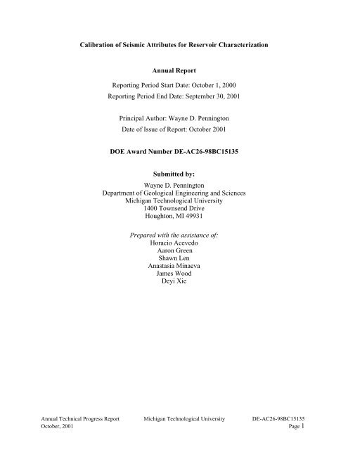
Calibration of Seismic Attributes for Reservoir CharacterizationAnnual ReportReporting Period Start Date: October 1, 2000Reporting Period End Date: September 30, 2001Principal Author: Wayne D. PenningtonDate of Issue of Report: October 2001DOE Award Number DE-AC26-98BC15135Submitted by:Wayne D. PenningtonDepartment of Geological Engineering and SciencesMichigan Technological University1400 Townsend DriveHoughton, MI 49931Prepared with the assistance of:Horacio AcevedoAaron GreenShawn LenAnastasia MinaevaJames WoodDeyi XieAnnual Technical Progress Report Michigan Technological University DE-AC26-98BC15135October, 2001 Page 1

AbstractThe project, “Calibration of Seismic Attributes for Reservoir Calibration,” has completed theinitially scheduled third year of the contract, and is beginning a fourth year at no additional cost,designed to expand upon the tech transfer aspects of the project. From the Stratton data set wehave demonstrated that an apparent correlation between attributes derived along ‘phantom’horizons are artifacts of isopach changes; only if the interpreter understands that theinterpretation is based on this correlation with bed thickening or thinning, can reliableinterpretations of channel horizons and facies be made. From the Boonsville data set wedeveloped techniques to use conventional seismic attributes, including seismic facies generatedunder various neural network procedures, to subdivide regional facies determined from logs intoproductive and non-productive subfacies, and we developed a method involving crosscorrelationof seismic waveforms to provide a reliable map of the various facies present in thearea. The Teal South data set has provided a surprising set of data, leading us to develop apressure-dependent velocity relationship and to conclude that nearby reservoirs are undergoing apressure drop in response to the production of the main reservoir, implying that oil is being lostthrough their spill points, never to be produced. The Wamsutter data set led to the use ofunconventional attributes including lateral incoherence and horizon-dependent impedancevariations to indicate regions of former sand bars and current high pressure, respectively, and toevaluation of various upscaling routines.Our work on these four data sets is now essentially complete, and our attention is focussed onnew tech transfer methodologies, including the use of tutorials and other examples on CD-rom aswell as conventional publications and presentations. The results of the Teal South data set havealready attracted some attention due to their implications for reservoir management andexploitation techniques.Annual Technical Progress Report Michigan Technological University DE-AC26-98BC15135October, 2001 Page 3

Table of ContentsDISCLAIMER............................................................................................................................... 2ABSTRACT................................................................................................................................... 3TABLE OF CONTENTS.............................................................................................................. 4LIST OF GRAPHICAL MATERIALS ...................................................................................... 6EXECUTIVE SUMMARY........................................................................................................... 9INTRODUCTION....................................................................................................................... 11TASK 1: PROJECT MANAGEMENT............................................................................................... 11TASK 2: BOREHOLE DATA ......................................................................................................... 11TASK 3: PROCESSING ................................................................................................................. 11TASK 4: VISUALIZATION............................................................................................................ 12TECHNOLOGY TRANSFER ........................................................................................................... 12RESULTS AND DISCUSSION ................................................................................................. 13STRATTON FIELD, SOUTH TEXAS............................................................................................... 13Background ........................................................................................................................... 14Phantom Horizon Technique ................................................................................................ 15Shallow channel region......................................................................................................... 17The Region of Gas Production.............................................................................................. 20Discussion ............................................................................................................................. 22Conclusions (Stratton Field)................................................................................................. 22BOONSVILLE FIELD 1: QUANTITATIVE SEISMIC FACIES ANALYSIS FOR THIN-BED RESERVOIRS .. 23Introduction........................................................................................................................... 23Well-Based Depositional Model ........................................................................................... 25Seismic trace pattern and Depositional Model..................................................................... 27Seismic trace coherence........................................................................................................ 27Seismic trace pattern classification ...................................................................................... 28A New Agorithm for Seismic Facies Analysis....................................................................... 29Conclusions........................................................................................................................... 31Annual Technical Progress Report Michigan Technological University DE-AC26-98BC15135October, 2001 Page 4

BOONSVILLE FIELD 2: SEISMIC ATTRIBUTES FOR THIN-BED RESERVOIR PREDICTION............... 32Introduction........................................................................................................................... 32Evaluation of the Conventional Thin-Bed Tuning Model ..................................................... 33Generalized Regression Neural Network Inversion.............................................................. 36Other Inversion Models ........................................................................................................ 39Constrained sparse spike inversion (CSSI)........................................................................... 41Conclusions........................................................................................................................... 42TEAL SOUTH, OFFSHORE LOUISIANA, GULF OF MEXICO ........................................................... 43Introduction and Field Characteristics................................................................................. 43Rock Properties Determination ............................................................................................ 45Pre-Stack Time-Lapse Seismic Observations ....................................................................... 47Implications........................................................................................................................... 49WAMSUTTER ARCH, WYOMING................................................................................................. 50Setting and Production Characteristics................................................................................ 51Sand Bar Identification: Lateral Incoherence ...................................................................... 52Fluid Pressures and Micro-Fracturing: DFM and Impedance Variation............................ 53Upscaling and Backus Averaging ......................................................................................... 56SUMMARY OF ATTRIBUTE CHARACTERISTICS............................................................................ 59CONCLUSIONS ......................................................................................................................... 60ACKNOWLEDGMENTS .......................................................................................................... 60REFERENCES............................................................................................................................ 61LIST OF ACRONYMS AND ABBREVIATIONS .................................................................. 63Annual Technical Progress Report Michigan Technological University DE-AC26-98BC15135October, 2001 Page 5

List of Graphical MaterialsFigure 1: Location of the Stratton Field (adapted from Hardage 1995). ...................................... 14Figure 2: Stratigraphic sequence of the Oligocene ....................................................................... 14Figure 3: Seismic section showing the two horizons studied. ..................................................... 15Figure 4: Calculating normalized trace gradients for the facies classification. ............................ 16Figure 5: The shallow channel region at approximately 842 ms in time...................................... 17Figure 6: Structural (time) surface of the picked horizon outlining the channel .......................... 18Figure 7: The phantom horizon created by subtracting 101 ms from reference horizon A.......... 18Figure 8: Attributes of the phantom horizon corresponding to the shallow channel.................... 18Figure 9: Unsupervised facies classification of the shallow channel region. ............................... 19Figure 10: Time structure on the F39 horizon. ............................................................................ 20Figure 11: Attributes on the phantom horizon corresponding to the F39 level. ........................... 21Figure 12: Seismic facies classification of the F39 Phantom horizon. ......................................... 21Figure 13: Horizons associated with tracking F39........................................................................ 21Figure 14: Isopach of time separation between the F11 horizon and the tracked F39 horizon. ... 22Figure 15: Sample impdeance contrasts in Boonsville field......................................................... 23Figure 15: Location map of the Boonsville study area. ................................................................ 24Figure 16. Traverse seismic line through the main delta showing the Caddo sequence............... 24Figure 17: Generalized well log trends and corresponding depositional...................................... 25Figure 18: Representative well log trends and depositional facies............................................... 26Figure 19: Well correlation and interpretation for depositional facies ......................................... 26Figure 20: Seismic coherence time slice at 890 ms within the Caddo sequence. ......................... 28Figure 21: Seismic trace pattern classification ............................................................................. 28Figure 22: Seismic facies based on new algorith, using one trace at a time for classification. .... 30Annual Technical Progress Report Michigan Technological University DE-AC26-98BC15135October, 2001 Page 6

Figure 23: The combined seismic facies using multiple traces. ................................................... 31Figure 24: Conventional thin-bed tuning model with notations for our data set. ......................... 33Figure 25: Modeled seismic response........................................................................................... 34Figure 26: Seismic features through the main delta system.......................................................... 34Figure 27: RMS Amplitude plotted against summed thickness of sandstone and limestone. ...... 35Figure 28: Inverted impedance curves using the GRNN model at 36 wells................................. 37Figure 29: Crosslines 171 (a) and 125 (b) of the inverted impedance data .................................. 38Figure 30: Inverted impedance volume (GRNN model) with different opacity cut-offs. ............ 38Figure 31: Inverted impedance data using the PNN model. ......................................................... 39Figure 32: Crossline 117 of the invertedimpedance volume using the PNN model..................... 40Figure 33: Actual sandstone and limestone thickness plotted against predicted .......................... 40Figure 34: Estimated sandstone thickness of Caddo main delta system (PNN model) ................ 40Figure 35: Traverse line showing the inverted impedance using CSSI model ............................. 41Figure 36: Inverted impedance volume using the CSSI with different opacity cut-offs. ............. 42Figure 37: 3D perspective view of the sand structure................................................................... 44Figure 38: Smoothed production history of the 4500-ft reservoir ................................................ 44Figure 39: Inverted (legacy data) volume showing acoustic impedance ...................................... 45Figure 40: Time-lapse difference mapped on the 4500-ft horizon .............................................. 45Figure 41: Changes in P-wave velocity (Vp), Poisson’s ratio (PR............................................... 46Figure 42: Predictions for Amplitude-versus-Offset effect. ......................................................... 46Figure 43: Amplitudes extracted from the partial-offset data for the 4500-ft reservoir ............... 47Figure 44: Amplitudes extracted from the partial-offset data over the Little Neighbor. .............. 47Figure 45: A traverse through the inverted acoustic impedance volume...................................... 48Figure 46: Cartoon schematic ....................................................................................................... 49Figure 48: (Approximate) location of the seismic survey............................................................. 51Annual Technical Progress Report Michigan Technological University DE-AC26-98BC15135October, 2001 Page 7

Figure 49: Typical logs of the portion of the Wamsutter field. .................................................... 51Figure 50: Seismic section in area of the sand-bar ....................................................................... 52Figure 51: Variance....................................................................................................................... 53Figure 52: Identification of zone investigated for lower acoustic impedances............................. 54Figure 53: Acoustic impedance volume........................................................................................ 54Figure 54: DFM volume. .............................................................................................................. 55Figure 55: Comparison of RMS amplitudes, acoustic-impedance, and DFM. ............................. 56Figure 56: Example of a log suite ................................................................................................. 57Figure 57: Original logged velocity function with the Backus-averaged log ............................... 58Figure 58: Conventional synthetic seismogram with our Hi-Fi Backus averaged ....................... 59Annual Technical Progress Report Michigan Technological University DE-AC26-98BC15135October, 2001 Page 8

Executive SummaryThe project, “Calibration of Seismic Attributes for Reservoir Calibration,” has completed theinitially scheduled third year of the contract, and is beginning a fourth year at no additional cost,designed to expand upon the tech transfer aspects of the project. We have completed allessential work on four major data sets and have made intriguing conclusions in all of them. Asthe preparation of tech transfer items continues, we expect to find minor additional tasks toperform on some of the individual data sets, for completeness or demonstration purposes.Our description of the work performed will follow each data set, and the discoveries madeassociated with them. A summary will present those same discoveries in terms of theirrelationship to the current state of the art in seismic calibration interpretation.The Stratton data set has provided a challenge in thin-bed reservoir characterization in theabsence of sonic-log calibration data. In general, the seismic character of potential productivezones is obscure in this data set, and horizons containing the pay zones are typicallydiscontinuous. Previous work by other authors has demonstrated the apparent usefulness ofsimple attributes mapped along ‘phantom’ horizons which were tied at one well through a VSPand controlled by a constant offset from a nearby continuously tracked horizon. We havedemonstrated in this project that this apparent correlation is an artifact of isopach changes, whichdominate the interpretations based on simple attributes and on seismic facies analysis. However,if the interpreter understands that the interpretation is based on this correlation with bedthickening or thinning, reliable interpretations of channel horizons and facies can be made.The Boonsville data set has provided another challenge in thin-bed reservoir characterization, inwhich the seismic character of a productive sand zone appears, indistinguishable from thecharacter of a non-productive limestone to most commonly used attributes. In this case, theinterplay of impedance and thickness conspire with tuning to produce the similarity in mostattributes. This problem was attacked with two methods. In the first method, a technique wasdeveloped that made use of the well-log interpretations to divide the area into a number of facies,following a reasonable geological model; then the seismic attributes, including seismic faciesgenerated under various neural network procedures, were used to further subdivide thoseregional facies into productive and non-productive subfacies. In the other method, a newtechnique involving cross-correlation of seismic waveforms was developed to provide a reliablemap of various facies present in the area; we think this technique holds great promise for otherdata sets as well, and it appears to be extremely robust.The Teal South data set has provided a surprising set of data, extremely rich in interpretationpossibilities. We used the limited log data and excellent seismic data of this class III AVO brightspot reservoir in the Gulf of Mexico to develop a robust seismic petrophysics model throughwaveform (stratigraphic) inversion for acoustic impedance. We then used this model, togetherwith a pressure-dependent elastic modulus relationship developed by us, to predict the futureseismic response of the reservoir, as it was produced. Our predictions met the observations withuncanny accuracy. But observations of nearby, unproduced reservoirs also indicated a similarresponse, one that was not predicted with classical reservoir models or simulations. Weconcluded that these nearby reservoirs are undergoing a pressure drop in response to theproduction of the main reservoir, and that oil is being lost through their spill points (as gas comesout of solution), never to be produced. This set of observations may have serious ramificationsfor engineering and exploitation techniques throughout the Gulf of Mexico.Annual Technical Progress Report Michigan Technological University DE-AC26-98BC15135October, 2001 Page 9

The Wamsutter data set provided our most-challenging opportunities. This thin bedded lowporositysand within the Almond formation of the western US has demonstrated to other studiesthat conventional seismic attributes are not typically useful in identifying depositional facies orproductive zones. We sought unconventional attributes that were designed to identify thosefeatures which we concluded should be in the seismic data as a result of knowing the rockphysics associated with production. We found that a measure of lateral incoherence, developedby us, and applied along a phantom horizon designed to track a sand bar and its distal marineequivalent, provided extraordinary correlation with productivity from that sand bar. We alsofound that a technique we developed to identify high pressure from impedance variations alonglayers correlates strongly with results from the DFM technique of TransSeismic International andwith zones of high production not associated with the sand bar; our interpretation is that thesetechniques are indicating zones of high fluid pressure and/or microfracturing. We also tested avariety of techniques of upscaling sonic and density logs to the seismic scale using the thin-layereffective medium model of G. Backus, and have significantly improved the tie between syntheticseismograms and real seismic data in this data set.The main results of the project can be classified along these lines:ƒ Pitfalls (how to use ‘phantom’ horizons carefully)ƒ Unconventional attributesƒ Lateral extent of incoherenceƒ Cross-correlation with ‘type’ seismogramsƒ Impedance variation within specific layersƒ Upscaling from sonic to seismicƒ Methodologyƒ Recommendations for routine implementation (under development)ƒ Pressure-dependence of elastic propertiesƒ New relations based on (existing, from Han) dry-frame laboratory measurementsƒ Importance of inclusion in time-lapse studiesƒ Reservoir behavior detected from time-lapse seismic observationsOur work on these four data sets is now essentially complete, and our attention is focussed onnew tech transfer methodologies, including the use of tutorials and other examples on CD-rom aswell as the conventional publications and presentations. The results of the Teal South data sethave already attracted some attention due to their implications for reservoir management andexploitation techniques.Annual Technical Progress Report Michigan Technological University DE-AC26-98BC15135October, 2001 Page 10

IntroductionThe objectives of this project are three-fold: To determine the physical relationships betweenseismic attributes and reservoir properties in specific field studies; to improve the usefulness ofseismic data by strengthening the physical basis of the use of attributes; and, in the third year ofthe project, to test the approaches suggested or developed during the first two years on at leastone new data set. In association with these studies, collaboration with corporate partners andtechnology transfer as ideas are developed and tested are ongoing integral components. We haveextended the project to a fourth year (at no additional cost) to implement new technology transfercomponents, including tutorials and other approaches.This report will summarize the current state of the various tasks of the project, following theProject Work Plan. Then it describes the results of our analyses of each data set in some detail.Finally, it summarizes the results and conclusions.Task 1: Project ManagementProject management encompasses reporting and project support. Reporting is on schedule.Project support is on schedule after some initial redirection of efforts during the first year(resolved by the hiring of additional support personnel in systems administration).Training for some of the software packages has been accomplished by attending training coursesconducted by the companies providing the software. To date, we have had members of our teamtake part in training on the following packages:• GeoQuest GeoFrame products• IC2 from Scott Pickford• Stratimagic from Paradigm Geophysical• Jason GeoScienceWe also use Landmark Graphics products, GXTechnology products, and Seismic Micro-Technology products.Task 2: Borehole DataBorehole data for this project consists of three types: existing log data, existing core data, andnew core data. We have made use of all existing data, and have obtained new information onwell-completion histories in Stratton field for help in identifying productive intervals in thiscomplex field. We made new measurements on existing core from the Wamsutter area to help incharacterizing the thin-bed nature of the formation. And we have made novel use of invertedseismic data to constrain rock properties where log data was incomplete.The Borehole Data task portion of this project is complete.Task 3: ProcessingWe have conducted most of the processing of data that is required at MTU using softwareprovided by donors; additional processing (for the DFM) has been conducted by a subcontractor.To date, our processing efforts have included the following:Annual Technical Progress Report Michigan Technological University DE-AC26-98BC15135October, 2001 Page 11

• prestack processing of multiple 2D lines to evaluate acquisition artifacts,• poststack processing for attribute extraction,• poststack processing for variance/coherence,• poststack inversion for acoustic impedance, and• synthetic seismogram generation.New routines have been written using MatLab or other languages appropriate to the task. Nosignificant additional processing is anticipated in this project, other than what may be required tosupport the technology transfer component.Task 4: VisualizationIn our project organization, visualization includes the massive effort of data management as wellas the specific techniques for visualization. We have been able to utilize the 3D visualizationcapabilities of our software packages for interpretation of the data we have processed, and haveput the processed (DFM) data volumes from a subcontractor (TransSeismic International) into a3D visualization package for easier interpretation.The software that we are using provides outstanding visualization capabilities, and we continueto develop approaches to viewing the data in ways (including animations and illuminations) thatmake interpretation and transfer of ideas straightforward. We continue to find new ways tovisualize the results of our work, and anticipate some additional effort in this area to support thetechnology transfer component.Technology TransferOur web site is complete and is updated regularly (http://www.geo.mtu.edu/spot). We presentedan oral presentation and posters at the annual AAPG meeting in Denver, CO in 2001, oralpresentations at the SEG meeting in Calgary in 2000, published an invited review paper on“Reservoir Geophysics” in GEOPHYSICS, 2001, and have a manuscript in press in THE LEADINGEDGE for October, 2001. We are working on at least four other publications and on noveltechniques for providing experiences in seismic calibration for interpreters.Annual Technical Progress Report Michigan Technological University DE-AC26-98BC15135October, 2001 Page 12

Results and DiscussionThis section of the annual report first describes current results for each data set, then discussesthese results and suggested interpretation as a whole.Stratton Field, South TexasThe public-domain data set from Stratton field has provided the challenge of imaging featuresbelow seismic resolution, in an effort to identify the channels known to be present in the volume.Some of the channels are readily seen, particularly at shallow levels, but most channels can onlybe inferred by correlation with well data and through recognition of subtle features on theseismic data.The Stratton field produces from the Frio formation from reservoirs contained within a series ofmeandering channel-fill deposits. The Texas Bureau of Economic Geology (BEG), in a projectsupported by the U. S. Dept. of Energy (DOE) and the Gas Research Institute, studied this fieldin some detail (e.g., Hardage et al., 1994), in an effort to use seismic data to aid in identifyingsources of reservoir compartmentalization. They also made a subset of the data available forpublic use. In their study, the BEG found that seismic data could resolve very small channels atconsiderable depth: down to 10 ft (3 m) thick, 200 ft (61 m) wide, at depths greater than 6000 ft(1800 m). They interpreted some channels in the time structures (assuming that they representpaleo-topographic surfaces along which the streams flowed). They were generally unable to‘track’ the specific horizon of interest in this thin-bedded environment, partly because not allhorizons were continuous, and partly because the geologic bed of interest (as indicated in welllogs) did not correspond to a clear peak or trough. They made extensive use of ‘phantom’horizons (our word, not theirs, but now in common usage), at a constant offset from readilytrackedhorizons, and tied at one well where a VSP was conducted.We have extended an approach used by the BEG to include a complete wave-shape matchingroutine rather than a simple point attribute at the VSP-controlled time of the reservoir bed. TheBEG approach is straightforward and readily accomplished on most workstation softwarepackages. The approach we are using has only recently become available. The technique wehave applied is implemented in the commercially available package Stratimagic, which uses aneural-network method to divide the wave shapes found in the interval being considered into a(user-specified) number of different ‘facies.’ The maps displaying the spatial locations of thedifferent facies can often provide a picture of geologically meaningful features, such as channelsor crevasse-splays. We pursued this approach because the BEG result indicates that subtledifferences in wave character provide strong clues to the location of channels or to thecompartmentalization of the reservoirs.Our observations and maps initially were similar to those obtained by the earlier studiesconducted by the BEG. However, our interpretation of the physical origin of the features onthese maps is significantly different from theirs. We have concluded that most of the featuresrecognized from these phantom horizons are in fact due to isopach differences between thephantom horizon and the local horizon; these may, in turn, be due to the presence of channels (inone case this is clear). But the attributes themselves are not directly associated with lateralchanges in horizon properties – instead, the ‘phantom’ horizon crosses true horizons as theinterbed thickness varies, and the determined attributes naturally change as these beds arecrossed. The details are presented in the following summary.Annual Technical Progress Report Michigan Technological University DE-AC26-98BC15135October, 2001 Page 13

BACKGROUNDThe Stratton field is located in South Texas approximately 30 miles southwest of Corpus Christi(Figure 1) in Kleberg and Nueces counties. The 2 square-mile migrated 3-D seismic volume,containing 100 inlines and 200 crosslines spaced at 55 feet intervals, sampled at 2 ms in time,has been provided by the Texas Bureau of Economic Geology (Hardage et al, 1994) togetherwith data from 21 well logs and one Vertical Seismic Profile (VSP). The data were acquiredusing an 8-120 Hz Vibroseis sweep. Like many gas fields with a long production history, the logsuites vary greatly among the wells. The wells were drilled from the 1950’s to the early 1990’sand generally were logged with gamma, resistivity, and neutron logs. Since sonic logs are notavailable for any wells in the field, we rely on a checkshot derived from the VSP. There are nolog data available for the nonproducing shallow channel region investigated here. We havereceived limited production data provided by the operator Collins & Ware.The major producing formations are the nonmarine fluvial Upper Vicksburg and Middle Frioformations (Figure 2). The Upper and Middle Frio contain nonmarine channels; the Lower Friohas been described as a coastal plain, and the Upper Vicksburg Formation is thought to be deltaicin origin. The Frio formation is comprised of thin-bedded sandstones and mudstones as thin as10 ft. A series of growth faults in the Vicksburg terminate at an unconformity at the base of theFrio. The horizons and growth faults are identified on a seismic section in Figure 3.In this study, we analyzed a shallow non-productive horizon containing an apparent channel, anda deeper productive horizon just above the Frio-Vicksburg unconformity.Figure 1 Location of the Stratton Field (adaptedfrom Hardage 1995).Figure 2 Stratigraphic sequence of the OligoceneAnnual Technical Progress Report Michigan Technological University DE-AC26-98BC15135October, 2001 Page 14

Conventional attributesTo better image the shallow channel and deeper producing horizons, conventional attributes werederived. Conventional attributes can be divided into point based and interval based attributes.Point based attributes include, but are not limited to, amplitude, instantaneous amplitude,instantaneous phase, and instantaneous frequency. These attributes are derived directly on ahorizon. Interval attributes involve using a time window based upon an interval of a horizon oran interval between a horizon. Calculations that involve averages over a given time window,such as RMS amplitude, are examples of interval based attributes.Facies classification techniqueThe term “seismic facies classification” can have many different meanings. For the purposes ofthis study, seismic facies classification is used to describe the process of grouping the traces of asurvey into a limited number of categories based on the shape of each trace over a fixed timewindow (Poupon et al, 1999). To perform a seismic facies classification, a horizon and a fixedtime window surrounding the horizon of interest should be chosen and the amplitudes extractedwith the associated times. For example, if a 12 ms interval is chosen, with a 2 ms sample rate,there will be 7 amplitude values at 0,2,4,6,8,10 and 12 ms in time within the window. Thesesamples are used to compute gradients by calculating the change of the value between samples(Figure 4). For this example, a list of 6 gradient values would be created. The series is thennormalized by dividing each value by the largest gradient value. The series can be thought of asa 6 dimensional vector with each dimension having a value ranging between minus one and one.These vectors are then obtained for every trace in the survey or area of interest. Next, a neuralnetwork process searches for clusters of these vectors, a process roughly equivalent to findingclusters of waveshapes. Each trace is then placed into a category or class, based on theseclusters. Each trace has been classified based on its normalized gradient vector, and it isprimarily the trace shape (changes in amplitude) that drives the classification rather than directamplitude values. The number of classifications will determine the resolution of the trace shapeanalysis. As more classes are used, smaller and smaller details will become visible in theanalysis, which are shown as color changes in a facies classification map, but the noise in theimage will also tend to increase. If more detail is needed, the survey can be subdivided intomultiple regions to improve the classification process. A smaller region will have fewer tracesand will need fewer classifications to provide the same amount of information.Figure 4: Calculating normalizedtrace gradients for the faciesclassification.The previous work performed byHardage et al (1994) limited theanalysis to point based amplitudeobservations. If a point basedamplitude analysis can giveinformation about a feature, thenperforming an analysis using theentire trace over a window of time can be expected to provide more details about that feature.Furthermore, if a single instance of time near a horizon can give useful information, using aAnnual Technical Progress Report Michigan Technological University DE-AC26-98BC15135October, 2001 Page 16

window of time above and below that horizon should be able to give even more information. Forexample, if the producing region is present either slightly above or below a horizon, utilizing atime window that includes these areas may show features that might have been missed if theattributes were calculated directly on a horizon. Examining the trace shape over the timewindow could provide clues to the inherent waveshape property or properties that are associatedwith the fluid content. Using neural network technology, the traces (over a certain window oftime) can quickly be divided and placed into a similar model trace, which can then be used toidentify structural features. Classifying the shape of the trace should allow the delineation ofmore detailed features over a region than using a single point based attribute. The more classesused, the fewer the number of traces in each class, and the more detailed the analysis.For the first example in the Stratton Field, a channel will be identified, and the faciesclassification technique will be used to later separate the traces based upon differences within thetrace.SHALLOW CHANNEL REGIONAn apparent channel at approximately 842ms can be located in the shallow region of the StrattonField. This channel is easily identified from amplitude measurements on a time slice (Figure 5),but a phase change is introduced across this time slice by the gentle dip of the beds.Figure 5: The shallow channel region at approximately 842 ms in time. A phase change occurs(from light to dark gray) across the image due to the gentle dip of the horizon.Conventional Attributes on the shallow horizonFigure 6 shows the time structure of the interpreted horizon containing the shallow channel.Although visible, the channel is not clearly represented on this structural time surface, becausethe channel is consistently about 2 ms later than neighboring traces on the horizon, yet thehorizon exhibits total relief (due to gentle dip) of about 40 ms obscuring the small timedifferences. Because the channel differs from the surrounding traces by only 2 ms, the effect ofthe dip must be removed to emphasize these differences. A number of additional attributes wereAnnual Technical Progress Report Michigan Technological University DE-AC26-98BC15135October, 2001 Page 17

extracted along this horizon, none of which provided a more clear indication of the channel thanthe time structure.Figure 6: Structural (time) surface of thepicked horizon outlining the channel.Conventional attributes using a phantom horizonA continuous horizon (found at 945 ms at well 9) was chosen and named reference horizon A(Figure 7). The time difference between the interpreted shallow channel horizon and referencehorizon A at well 9 is 101ms. The time difference was chosen to overly the non-channel faciesover most of the survey area. The new phantom horizon was created with the intention ofremoving the general dip structure from the shallower horizon. Attributes were then calculatedover this phantom horizon, some of which are shown in Figure 8. Both the amplitude slice andRMS amplitude (which was calculated over a 20 ms window of time centered on the phantomhorizon) do an excellent job of defining the channel, largely because the phantom horizon gentlyaccounts for the dip, while cutting across the channel feature.Figure 7: The phantom horizoncreated by subtracting 101 msfrom reference horizon A.Left side: Time. Center: Amplitude. Right: RMS AmplitudeFigure 8: Attributes of the phantom horizon corresponding to the shallow channel.Annual Technical Progress Report Michigan Technological University DE-AC26-98BC15135October, 2001 Page 18

Facies Classification of shallow channel regionThe final approach applied to the channel horizon makes use of the facies classificationtechnique. A 20ms time window centered on the phantom horizon was chosen to perform thetrace shape analysis. An unsupervised neural network with 14 classifications produced theimage shown in Figure 9a.The relatively clear boundaries emphasize the sinuous form of the channel. Figure 9b shows themodel traces used to create the classification. Notice that a gradual time shift of the wavelets hasoccurred with approximately a 1 ms shift from one classification to the next. The channel isrepresented by the 13 th and 14 th classifications shown as dark blue and purple colors on the faciesmap. In effect, the trace shape of the channel has been classified by a small time delay; thefacies classification technique is highly sensitive to time shifts.Figure 9: Unsupervisedfacies classification of theshallow channel region.9a (upper figure) showsthe classification, andfigure 9b (lower) showsthe wavelets used in theclassification.Discussion of the shallow channel regionIn the shallow region, both point-based amplitude attributes and the interval attributes were noteffective in imaging the channel when performed directly on the tracked horizon. The phantomhorizon permitted much better identification of the channel than the original horizon, primarilydue to the time shift involved. That is, because the channel reflection arrives about 2 ms laterthan the surrounding non-channel horizon, the phantom horizon encounters a slightly differentphase at the location of the channel, and its amplitudes are correspondingly affected. Thedifference results in the dramatic color contrast between the feature and the surrounding survey.It is this color change that allows the viewer to separate the channel from its surroundings.Annual Technical Progress Report Michigan Technological University DE-AC26-98BC15135October, 2001 Page 19

The seismic facies classification technique based on trace shape works for similar reasons. Eachtrace is classified as a multidimensional vector, with time shifts having a large impact upon theclassification. The small time shift results in model traces created by the neural network thatspecifically image the channel. To image structures with small time changes, both phantomhorizons and facies classification techniques based on trace shapes can be effective, but the usershould recognize that the classification based on a phantom horizon may simply be due toisopach differences between the features being identified and the reference horizon.THE REGION OF GAS PRODUCTIONFor the second portion of the study of the Stratton field, we attempted to image a much moresubtle case in the deeper region of production. Assorted well logs and limited productioninformation are available for this region.In the Stratton field, the F39 horizon is one of the primary producing intervals and appears on theseismic data at approximately 1640 ms in time. Unlike the channel horizon (tracked onminimum amplitude or trough), the F39 horizon was tracked using a maximum (peak)determined from times provided in Hardage et al (1994) at each of the well locations. Figure 10shows the time structure of this horizon; we see a gently arching structure across the survey. Asin the previous examples of the shallow region, amplitude, RMS amplitude, and instantaneousfrequency were unable to decisively identify any channel or potentially productive zones. Aphantom horizon was therefore created to better image this region.Figure 10: Timestructure on theF39 horizon.Conventional attributes using a phantom horizonThe F39 horizon was difficult to track due to tuning effects. The phantom horizon techniqueused by Hardage et al (1994) was reproduced here: the F11 horizon was tracked and a phantomhorizon was created at the level of the F39 horizon at the VSP well (59 ms later; see Figure 3,presented earlier). We then calculated attributes over this phantom horizon. Figure 11 shows theamplitude and RMS amplitude calculated on this phantom horizon. Examining these attributesshow strong north-south linear features, and one may be tempted to conclude that these representstratigraphic differences in the F39 horizon.Annual Technical Progress Report Michigan Technological University DE-AC26-98BC15135October, 2001 Page 20

Left: AmplitudeRight: RMS AmplitudeFigure 11: Attributes on the phantom horizon corresponding to the F39 level.Facies classification of the deeper producing regionUsing the Facies classification technique on the phantom horizon and a 25ms time window (20ms above and 5 ms below), we see a dramatic time shift in the classifications (Figure 12).Investigating these features more closelyyields surprising results. These linearfeatures are not channel regions or areas offaulting as might be expected; they areareas (see Figure 13) where the true reliefof the F39 horizon is much greater than thatof the phantom horizon. The linear featuresare caused by the phantom horizon passingthrough alternating peaks and troughs.Figure 12: Seismic facies classification ofthe F39 Phantom horizon.Figure 13: Horizons associated withtracking F39.Red Horizon: F11, used for referenceGreen Horizon: Tracked F39 horizonYellow Horizon: Phantom F39horizon, based on the F11 referenceAnnual Technical Progress Report Michigan Technological University DE-AC26-98BC15135October, 2001 Page 21

To better portray the area between the F11 and tracked F39 horizons, an isopach map wascreated. Figure 14 shows that the isopach thickens to the west from 29 ms to 66 ms in time.These two horizons are not conformable and do not have the same dip; therefore, a phantomhorizon based on a constant time difference is not advisable.Figure 14: Isopach of time separation betweenthe F11 horizon and the tracked F39 horizon.DISCUSSIONTo deal with the difficulties posed by non-conformable and/or dipping beds, we offer twosuggestions. First, choose a reference horizon that is highly conformable to the horizon ofinterest. Most often this will be a horizon that is closely adjacent to the interpreted horizon. Anisopach map showing the time differences between the reference horizon and the poorly trackedhorizon of interest will aid in determining the degree to which the two horizons are conformable.In some cases, as in the F39 horizon, there are no nearby conformable horizons. Therefore,attributes must be calculated directly from the poorly-tracked horizon. We suggest using awaveshape-based facies classification scheme. As with the channel horizon, the graduallyincreasing time separation of the peaks is the driving force behind the classification. The traceshape analysis is very sensitive to time shifts caused by thickening or thinning of the nearbyhorizons. In the case of the deeper producing region, even anchoring on the horizon to beclassified, resulted in a classification based on stratigraphic thickening.Our second suggestion is to create proportional slices between the two horizons. This wouldwork best for regions that do not have nearby conformable reference horizons. Two horizons,bracketing the poorly-tracked horizon of interest, can be used to create a set of proportionallyinterpolated horizons, which can be used, as phantom horizons that may be fairly conformable tothe intermediate beds. These proportional slices will be less affected by conformable horizonssince the medial slices will be used. Measuring amplitudes over these proportional slices mayprovide an alternative approach to horizon slicing.CONCLUSIONS (STRATTON FIELD)The use of phantom horizons can provide strong assistance to the geophysical interpreter,particularly in areas where the level of interest does not correspond directly to a trackable event.The use of seismic facies classification schemes can provide additional strong assistance. Butboth approaches depend strongly on the phantom horizon’s conformability with the horizon ofinterest. If the events are not conformable, attributes extracted along the phantom horizon willcorrelate more strongly with isopach differences than with true formation properties within aspecific layer. On the other hand, if the interpreter recognizes these attributes as such, thephantom layer and its attributes can serve as a proxies for those geologic features that cause thethickening or thinning, but it is essential that the interpreter recognize them as such.Annual Technical Progress Report Michigan Technological University DE-AC26-98BC15135October, 2001 Page 22

Boonsville Field 1: Quantitative seismic facies analysis for thin-bed reservoirsIn this section, we describe a new pattern recognition model developed to recognize the subtlegeological and geophysical features of a thin-bed sequence and predict thin-bed reservoirs, basedon cross-correlation of seismic traces with one or more traces believed to represent specificdepositional environments. Our approach has the following characteristics: (1) It corrects for thepossible mistracking of top horizons by searching about a time window specified by the user; (2)It presents seismic facies as continuous values by introducing the modified cross-correlationalgorithm, as opposed to a limited number of clusters; (3) It more easily performs one or moresupervised trace pattern recognition and combines each of them into a seismic facies.INTRODUCTIONUsing 3-D seismic data integrated with well data to build reservoir depositional model is routinework and seismic stratigraphy plays a significant role, albeit in a qualitative fashion. However, itis not uncommon for thin sequences to exhibit seismic trace pattern changes that are subtle andwith ill-defined termination patterns. Our case study area poses an additional challenge: how todistinguish thin-bed reservoirs and thin-bed non-reservoirs when they appear similar at seismicscale. It is this second challenge that we address in this section.The average acoustic impedances of the shale, sandstone, and limestone of the Boonsville Fieldare 30000, 36000 and 40000 ft/s*g/cc respectively (Figure 15), indicating that we could separatethe sandstone reservoirs from the limestone non-reservoirs if we were capable of identifyingtheir acoustic impedance with any confidence. However, the discrimination is very difficult inthis field because the limestone and sandstone layers appear similar at the seismic scale.Figure 15: Sampleimpedance contrasts inBoonsville field.The fast bed at about 870 mstwo-way time is limestone,and the fast bed at 878 ms isa sandstone; the otherformations are mostly shales.The original impedance isshown in blue on all traces,and the filtered impedance isshown in red, using a highcutfilter as labeled. Noticethat below 120 Hz, thedistinction between thelimestone and sandstonebeds is insignificant.A sonic well log has a resolution less than 5 feet in comparison with seismic resolution, up to 50feet for the Boonsville data set. The frequency bandwidth of the Boonsville 3-D seismic data isfrom 15 to 120 Hz while the frequency bandwidth of the velocity log ranges from 0 to greaterthan 500 Hz. High-cut filtering is required to “upscale” the frequency bandwidth of the well datato the seismic data. As a result of high-cut filtering, the high impedances of the thin-beds areAnnual Technical Progress Report Michigan Technological University DE-AC26-98BC15135October, 2001 Page 23

averaged with nearby lower impedances. The final effect is that the higher impedance of thelimestone non-reservoir appears to be close to the impedance of the sandstone reservoir. A morecomplete treatment of the problem would include Backus (1962) averaging of the thin beds, withdetails depending on the frequency content of the wavelet, but the net effect will still be theoverall reduction of the highest impedance resolved. [This approach is considered later in thisreport, with the Wamsutter data set.] Therefore, two rock types may easily appear similar atseismic scale and become difficult to distinguish through the interpretation of a seismic data setalone, even though the actual thin-bed impedances are significantly differentOur study area is the Boonsville Field of the Fort Worth Basin in north central Texas (Figure16a). The data set includes 5.5 square miles of 3-D seismic data set and 38 wells with modernlogs , made available through the Texas Bureau of Economic Geology (Hardage et al., 1996a).Here we concerned ourselves within the Caddo sequence of the Pennsylvanian Group (Figure16) although other productive sequences also exit in the area.Figure 16a: Location map of the Boonsville study area.Figure 16b. Traverse seismic line through the maindelta showing the Caddo sequence.The reservoir characteristics and therelated data set meet our basic requirements to ensure reaching the research goals. Some featuresof the targeted Caddo sequence are: hydrocarbons are produced from the thin-bed sandstonereservoirs with thicknesses totaling 0 to 52 net feet of the Caddo sequence, with a gross thicknessof 80-150 feet; the tight limestones have known thicknesses of 0 to 30 feet and appear similar tothe thin-bed sandstones at seismic scale; the depositional environment is dominated by a deltasystem; both the sandstone and limestone are embedded in the shale-rich sequence andcharacterized by higher P-wave velocities and higher densities, thus generating higher acousticimpedances; both the sandstones and limestones are highly variable laterally and vertically.Our primary research goal is to establish a depositional model of the thin Caddo sequence usingthe 3-D seismic data integrated with well data. In this study, we first build a depositional modelusing the well data only, and then examine some existing approaches to the use of seismic datafor facies analysis, such as trace coherence and classification. A new method will be presented torecognize the subtle geological and geophysical features of the Caddo sequence, based on crosscorrelationof seismic traces with one or more traces believed to represent specific depositionalenvironments.Annual Technical Progress Report Michigan Technological University DE-AC26-98BC15135October, 2001 Page 24

WELL-BASED DEPOSITIONAL MODELThe depositional system of the Pennsylvanian Atoka Group has been studied by Thompson(1982; 1988), Glover, (1982), and Lahti et al. (1982). However, these studies were mainlyfocused on the entire Fort Worth Basin. Hardage et al. (1996b; 1996c) and Carr et al. (1997)analyzed the reservoir distribution and depositional subfacies using a few typical wells from thisstudy area, but their model is not sufficiently detailed to be useful for facies analysis of this thinCaddo sequence. In addition, the tight non-reservoirs were generally not studied even thoughboth the limestones and reservoir sandstones exist and appear seismically similar in theBoonsville Field. Therefore, a depositional model was established with a concentration onreservoir distribution and the discrimination of the sandstone from the limestone. The techniquesinvolved include well log trend recognition and lithology determination.The well log trends and lithologies analysis are summarized in Figure 17 and the well log trendsfrom representative wells are illustrated in Figure 18. The main delta system was recognized inthe east and the possible second delta system was observed at the northwestern corner, butappears to be mostly outside of the study area (Figure 18). The main delta system was dividedinto three delta subfacies: distal channel in the east margin, proximal delta front in the east, distaldelta extending to south and northeast, and interdelta in the south and southeast. As depicted in across-section through the main delta system (Figure 19), the depositional subfacies and reservoirdistribution in the eastern oil producing region are characterized by the distal channel and theproximal delta front are the depositional subfacies in which the thickest sandstone reservoir (upto 52 ft) was deposited; the distribution of limestones is limited, but the limestones can becorrelated as the GR log trend is similar and correlative; the sandstone reservoirs are widelydistributed in the delta front subfacies.Figure 17: Generalized well logtrends and correspondingdepositional subfacies andlithologies of the Caddosequence.(Modified from Coleman et al.,1982; Thompson, 1982; Emeryet al., 1996; Hardage et al.,1996b,; and Carr et al., 1997)Annual Technical Progress Report Michigan Technological University DE-AC26-98BC15135October, 2001 Page 25

Figure 18: Representative well log trends and depositional subfacies of the Caddo sequencebased on well data, with a possible limestone shelf and distributary channel based on seismicinversion. Cross-section A-B is indicated by the dashed line, and used in other figures.The second delta system observed from the well data was detected at the northwestern corner.However, the main delta body remains outside the study area (Figure 18) and the relationship ofthis delta system (or sub-system) with the main delta system (or subsystem) in the east remainsunclear.Figure 19: Wellcorrelation andinterpretationfor depositionalsubfacies andlithology; thewell section hasbeen flattenedon the BottomCaddo marker.Annual Technical Progress Report Michigan Technological University DE-AC26-98BC15135October, 2001 Page 26

The rest of the region is dominated by the prodelta or shelf, filled with shales and limestones.The SP log trend is a flat base line while the GR log pattern is a “boxcar”. The “boxcar”indicates the prodelta limestone. No good reservoir sandstone was found in the prodeltasubfacies, and instead, the shaly sandstones were recognized and no oil was produced from them.The maximum known thickness of the limestone in prodelta subfacies is 30 feet at well BY11and BY13. However, the simulated acoustic impedance data reveals that a narrow north-southorientedthicker limestone zone might exist in the west that will be discussed later.SEISMIC TRACE PATTERN AND DEPOSITIONAL MODELChen et al. (1997) suggested that more than 20 seismic attributes (not all of them areindependent) would be useful in constructing reservoir depositional model. Other researchers(Horkowitz, et al., 1996; Hardage et al., 1996b; Cooke, et al., 1999) claimed that instantaneousfrequency and/or instantaneous phase are effective at highlighting facies changes. Similarityanalysis based on multiple point-based attributes, their means and deviations was used to mapseismic facies (Michelena, et al., 1998). However, these point-based attributes only describe oneaspect of a complicated seismic trace shape. The trace-based attributes may be a natural solutionfor better defining facies. In this study, two widely used approaches, coherence and trace patternclassification will be examined before a new technique is presented and tested.Like the well-log trend, seismic trace pattern can be used to define a depositional facies. Noticethat the patterns of the synthetic traces created from velocity and bulk density well logs do notperfectly match the real seismic traces because of different measurement scale, assumptions, andnoise involved. However, they indicate that different depositional subfacies and reservoirdistribution correspond to the changes in seismic trace patterns, which is the petrophysical basisfor using seismic trace pattern to construct depositional subfacies.SEISMIC TRACE COHERENCESeismic trace coherence is a measure of lateral changes in the seismic trace pattern and is basedon a cross-correlation measurement. Bahorich et al. (1995) invented this technique and has sincebeen modified by introducing semblance, structural dip and azimuth (Marfurt et al. 1998; 1999).Bahorich et al. (1995), Marfurt et al. (1998; 1999), Cooke (1999), and Chopra (2001)demonstrated that coherence can be used to define stratigraphic features. Our study suggestedthat the resolution depends upon the scale and the degree of variations in the patterns ofneighboring traces. In particular, coherence may not be helpful if the changes in the patterns ofneighboring traces are gradual, in which case, all of the coherence values are almost identicaland no features are apparent. Furthermore, because the algorithm compares the neighboringtraces along inline and crossline directions or traces in small regular-shaped (elliptical orrectangular) analysis regions (tessellations) at each iteration, it cannot use specific traces forcorrelation through the volume.A coherence cube from the Boonsville data set was obtained (Figure 20). The delta depositionalfeature has not been recognized because its variations are subtle; on the other hand, the effects ofsome deep karstic features are apparent in the coherence volume, even at the Caddo level. Asexpected, the stratigraphic or structural features stand out if the changes are sharp. Wheneverthis is the case we can interpret them in a conventional reflection data volume, provided that acoherence cube makes these features more visible for interpretation. Overall, coherence seems tobe most useful in configuring depositional systems which involve significant changes in seismictrace pattern, and in interpreting structures because structural deformation often sharply distortsseismic trace patterns.Annual Technical Progress Report Michigan Technological University DE-AC26-98BC15135October, 2001 Page 27

Figure 20: Seismic coherence time sliceat 890 ms within the Caddo sequence.SEISMIC TRACE PATTERN CLASSIFICATIONThis approach classifies all seismic traces in a survey to a limited number of classes usingmathematical algorithms which vary from conventional cluster analysis to neural networkclassification. One popular algorithm is based on Kohonen self-organization map (SOM) neuralnetwork recognition (Kohonen, 1990; Gurney, 1992). Poupon et al. (1999) demonstrated itsusefulness in seismic facies analysis. Basically, in this scheme, each of the model classescorresponds to a discrete class of patterns and the problem then becomes a decision process. Allmodel classes are “self-organized” and updated at each iteration. The final classes are assigned toeach trace, each of them is labeled with the corresponding model classes or colors (the lowerpanel in Figure 21). Notice that changing the time of first sample in the series, due to horizonmistracking, can significantly alter the vector value.ThickerlimestoneThickersandstoneFigure 21: Seismic trace patternclassification and correlateddepostional subfacies of the Caddosequence (upper panel) and ten tracemodel classes for the seismic traceclassification (lower panel, 30 mswindow from the top Caddo).interdeltaMain delta systeminterdeltaThe number of model classes for theneural network needs to beoptimized by maximum differenceamong each model class andmaximum correlation factor. Five,ten, fifteen, and twentyclassifications were initially chosenwith 30 ms tine window, and the tenclassificationresult provided a mapthat correlated best as the correlationfactor is greater than 70% in most ofthe study area. The patterns can becorrelated to the depositionalsubfacies (upper panel in Figure 21)Annual Technical Progress Report Michigan Technological University DE-AC26-98BC15135October, 2001 Page 28

if properly calibrated from the well data (Figure 18). Patterns 4-10 were correlated to the deltafront and patterns 9-10 were compared to the inter-delta subfacies, patterns 4-8 to the prodeltasubfacies. Patterns 5-6 in the west represent thicker limestone zone in the prodelta subfacies.Again, notice that each of the pattern groups is meaningful with depositional subfacies becausethey were properly correlated to the well-based depositional subfacies.A NEW AGORITHM FOR SEISMIC FACIES ANALYSISWe developed a new approach which can: (1) realign a mistracked horizon, (2) discern subtlechanges in seismic trace patterns, (3) easily perform pattern recognition for user-specified tracesover a survey, (4) provide continuous output values, and (5) combine and visualize the results formultiple trace pattern analysis (posterior-classification).The algorithm is a modified cross-correlation model, which is a standard method for estimatingthe degree to which two series are correlated. Consider two series of signals X(i) and Y(i) wherei = 1, 2, … N. The cross-correlation, R, at delay d is defined asR =∑NiN∑i[( X ( i)− X( X ( i)− Xm)2m)( Y ( i − d)− Y )]∑Nim( Y ( i − d)− Y )where X mand Y mare the means of the corresponding series and d is the time window for possiblehorizon mistracking. The denominator in the expressions above serves to normalize thecorrelation coefficients such that it ranges from –1 to 1. A value of one indicates maximumcorrelation while zero indicates no correlation. A high negative correlation exhibits a highcorrelation but of the inverse of one of the series. However, this cross-correlation is focused onthe relative similarity of patterns between two time series rather than absolute similarity. Hence,this expression was modified such that it can judge the difference in absolute values within theshape. The modified expression is written below, showing an additional factor that computes forsimilarity of amplitude on an absolute value:⎛⎜R =⎜⎜⎜⎝∑NiN∑i[( X ( i)− X( X ( i)− Xm)2m)( Y ( i − d)−Y∑Nim)]m( Y ( i − d)−Ym2)2⎞⎛⎟⎜⎟⎜⎟⎜⎟⎜⎠⎝N∑iN∑i⎞| Y ( i)| ⎟⎟⎟| X ( i)| ⎟⎠This algorithm, as implemented, can also correct for possible horizon mistracking by searchingan amount of time (d samples specified by the user) in order to find the highest value for R. Theoutput values for R are continuous from –1 to 1 and provide a value at every trace.The input of this model consists of seismic data and horizon file as provided by the user. Theuser needs to define the possible mistracking time window which depends on the confidence ofthe horizon tracking. The users must then input a trace location of interest, usually a trace at awell with known lithology and/or depositional subfacies. The program will perform patternprocessing and output the results, indicating the similarity of all other traces to the one specifiedtrace. Results for one trace at a time are shown in Figure 22.Annual Technical Progress Report Michigan Technological University DE-AC26-98BC15135October, 2001 Page 29

Figure 22: Seismic facies based on new algorithm, using one trace at a time for classification.Upper left: based on well AC3.Upper right: based on well CWB21-1.Lower left: based on well IGY31 Lower left: based on trace Inline 76, Crossline 142In general, one-trace pattern recognition provides a good seismic facies map as shown in Figure22 derived from well AC3 only, with R values ranging from –0.8 to 1. Three seismic facies typesare readily identified, and by consulting the well-based depositional model (Figure 18), theassociation with geological facies can be determined with ease. The area of the map with R-valuecorrelation above 0.7 indicates that all the trace patterns are close to the trace pattern at wellAC3, which is indicative of the main delta system (notice that the trace patterns were distorted atthe northeast corner where karst and faults were developed). Two isolated areas in which thecorrelation is low or negative indicate the inter-delta subfacies. The coefficient in the north isalso low, ranging from –0.3 to 0.7, and is correlated to the prodelta subfacies. Notice that thetime window used for the pattern processing is 30 ms starting from the top Caddo sequence, thesame size as the previous trace classification window.Various traces at different well locations were chosen to provide trace pattern processing fordifferent depositional facies. Well CWB21-1, also indicative of the main delta system was used,and the results are almost identical to the facies map derived from well AC3. Well IGY31recorded the inter-delta subfacies and its corresponding seismic trace pattern correlation resultsare consistent with the well-based map. Notice that other high coefficient values in the centralnorth area were detected where structural deformation (i.e., karst) was also identified with astrong correlation to this well, a result that is perhaps coincidental.This algorithm enables us to process any trace specified by the user, whether or not it is at a welllocation. The trace at inline 76 and cross line 142 is believed to be located within the thickerlimestone zone. The high coefficient values indicate the thicker limestone distribution in theAnnual Technical Progress Report Michigan Technological University DE-AC26-98BC15135October, 2001 Page 30

west. Notice that the trace patterns in the east where the thicker sandstone reservoirs weredeveloped also correlate with the limestone-based trace. Our algorithm can now be extended tohelp remove this apparent ambiguity.Although this new approach is capable of producing reliable seismic facies maps using only oneseismic trace for pattern processing, the results from multiple user-specified trace patternprocessing can be combined and visualized. The following expression is used to meet this need.R = i * max(R 1, R 2, …R i, …, R n)where i is the order of seismic trace chosen to perform the processing and n is the number of thetraces selected. R iis the correlation coefficient based on the selected trace with the order of i, thatis, R 1may be the correlation coefficient for a trace exemplifying the main delta, whereas R 2represents the inter-delta, R 3the limestone, and so no. The resulting R is then chosen as thatvalue, the largest from among the correlations made; it is also assigned a value (i) identifyingwhich facies it represents.Figure 23: Thecombined seismic faciesusing multiple traces.Left: traces at 3 wells.Right: limestone andsandstone traces added.Figure 23 depicts the combined seismic facies obtained from three pattern-processed seismictraces, that is, the traces at well AC3, IGY31 and BY11. These three wells represent the maindelta, inter-delta, and prodelta depositional subfacies, respectively. The figure also demonstratesthe ability to discriminate the thicker sandstone reservoirs in the east and thicker limestones inthe west by adding the additional facies from traces in the known limestone region and thicksandstone region.CONCLUSIONSThe seismic trace coherence may not able to reveal subtle depositional facies in a thin sequencebecause of gradual changes of the patterns among the closest neighboring traces. The traceclassification approach based on the neural network clustering provided very good results. Ournew approach appears to provide some advantages. It provides pattern recognition for multipleuser-specified traces (for example, specific “depositional trace” or “oil trace” and “gas trace”)over an entire survey. The algorithm has been demonstrated, via the case study, to be robust andpromising in defining seismic facies of subtle geological features and predicting thin-bedreservoirs. Notice that, similar to every geophysical output, the geological meaning needs to bedefined or verified by geological information. The same correlation values may not represent thesame depositional subfacies and the assignment of depositional subfacies depends on ourconfidence on the geology. More wells, if available, should be selected for the multiple tracepattern processing in those less confident regions.Annual Technical Progress Report Michigan Technological University DE-AC26-98BC15135October, 2001 Page 31

Boonsville Field 2: Seismic Attributes for Thin-bed Reservoir PredictionThe conventional thin-bed tuning model (i.e., the wedge model) is examined with emphasis onits usefulness or possible pitfalls in thin-bed reservoir prediction of the Caddo sequence, and anew non-linear statistical inversion model built on the generalized regression neural network(GRNN) is applied to the Caddo sequence. Two other seismic inversion models, a non-linearstatistical model based on the probabilistic neural network (PNN) and a deterministic modelusing constrained sparse spike inversion (CSSI) are used to delineate the reservoirs of the Caddosequence. Our study shows: (1) The conventional thin-bed tuning model is appropriate only ifone single thin-bed is developed or multiple widely-spaced thin beds (greater than one quarter ofthe wavelet length) are present in the sequence of interest. In other words, the model should notbe applied for multiple closely-spaced thin beds because of significant destructive interference;(2) All three seismic inversion models were able to identify the thicker reservoir sandstones.However, the resulting details for the thin beds vary. The sparse spike inversion with constraintsprovided few indications of the thin-bed distribution although it was largely noise-free. Theprobabilistic neural network (PNN) delineated most of the thin-beds, but produced more noise aswell. Our GRNN method predicted the thin beds at 13 out of 20 wells. The GRNN inversionmethod can be very useful in detecting thin-bed reservoirs in existing fields where a number ofwells are available.INTRODUCTIONReservoir characterization has historically focused on thick reservoirs (i.e., the thickness greaterthan seismic resolution). One of the most challenging research problems is to characterize thinbedreservoirs using 3-D seismic and well data. Based on the quarter wavelength criterion, thinbedreservoirs range in thickness from a few feet to tens of feet. Tuning effects are observed atthis thickness range due to wavelet interference (Widess, 1973; Brown, 1996) and thin-bedreservoirs may not be detected in seismic data or may be difficult to integrate with well data.However, thin-bed reservoir characterization is important as the petroleum industry is devotinggreater effort toward tapping more oil from existing fields, many of which are in thin-bedenvironments.Progress is being made towards characterization of thin-bed sandstone reservoirs using: (1)instantaneous seismic attributes (Hardage et al. 1994, 1996a; Horkowitz et al., 1996); (2)amplitude (Cooke et al. 1999; Hoover, 1999); (3) frequency decomposition (Partyka et al.,1999); and (4) Bayesian simulation (Gastaldi et al., 1998). To characterize thin-bed reservoirs,however, there are two key factors need to be taken into consideration. One is that a singlereservoir layer or multiple widely-spaced reservoir layers are rarely developed in a sequence ofinterest. Closely spaced thin-bed layers are difficult to predict using the conventional thin-bedtuning model which was generated for a single thin bed between two thick beds. The second oneis to remove the tuning effects (detuning). Reflections result from the convolution of a sourcewavelet with a reflection coefficient, thus representing the boundary between two layers insteadof the layer properties. Seismic inversion, which minimizes tuning effects or takes tuning effectsinto consideration, appears to provide a more robust approach for characterizing thin-bedreservoirs and is the subject of ongoing research (Salleh et al., 1999; Torres-Verdin et al., 1999;Riel, 2000; Pennington, 2001).Two approaches can be used to recover acoustic impedance from seismic data. One technique isto remove or minimize the tuning effects by applying a deconvolution model. This is theconventional deterministic seismic inversion. A few theoretical methods have emerged sinceAnnual Technical Progress Report Michigan Technological University DE-AC26-98BC15135October, 2001 Page 32

1980s, such as linear programming (Taylor et al., 1979; Cooke, et al., 1983; Oldenburg et al.,1983), maximum-likelihood or sparse spike inversion (Chi, et al., 1984), and more recently,constrained sparse spike inversion (Debeye et al., 1990). All these methods resolve thecomponents of the convolutional model in each seismic trace.The other alternative is to not remove the tuning effects from a seismic data set, but to establish astatistical relationship between seismic attributes and impedance (multi-attributes analysis,Hampson et al., 2001). Non-linear statistics are used to describe the relationship betweenattributes and acoustic impedance as the relation between them is complicated. Neural networksare most often used to construct this non-linear relation. A couple of neural networks that havebeen in use for seismic inversion are the multi-layer feed-forward neural network (MLFN) (Liu,et al., 1998) and probabilistic neural network (PNN) (Hampson, et al., 2001). Non-linearrelationships imply that more than one step or expression is required to simulate the observationsfrom the known inputs, in contrast to one step in linear relationship. Each layer consists of nodesand weights. The nodes are connected with weights and the neural network process finds theoptimal weights between the nodes by training a data set. Then, the statistical model is appliedto simulate an entire data set.Our study area is again the Boonsville Field, Fort Worth Basin of the north central Texas. In thisstudy, we examine the conventional thin-bed tuning model, apply a new generalized regressionneural network model, and perform a comparison study with two other inversion models with afocus on the prediction the thin-bed reservoirs.EVALUATION OF THE CONVENTIONAL THIN-BED TUNING MODELThe conventional thin-bed tuning model was derived from a wedge model. Widess (1973)demonstrated the interaction of the top and base reflectors of a thin bed wedge, illustrating thatamplitude increases as thin-bed thickness increases until the amplitude of the composite waveletreaches a maximum for a bed thickness of one-quarter wavelength. Clearly, the bed thickness atwhich these phenomena occur depends on the shape of the wavelet or its frequency band and thevelocity of the reservoir of interest. For instance, one-quarter of the wavelength is approximately50 feet for the Boonsville Field data set, given 12000 ft/s as the average velocity of the Caddosequence and 57 Hz as the dominant frequency of the seismic data (Figure 24). It is assumed thatthe post-stacked (summed) amplitude represents the zero-offset amplitude; that is, AVO effectswere ignored.Figure 4: Conventional thinbedtuning model withnotations for our data set.The thin-bed tuning modelhas been widely employed topredict thin-bed reservoirs.A number of case studieshave been published duringthe last decade (Brown, 1996;Hoover et al., 1999; Cooke etal., 1999). In reality,however, a sequence ofAnnual Technical Progress Report Michigan Technological University DE-AC26-98BC15135October, 2001 Page 33

interest is rarely developed by a single reservoir layer or by multiple widely-spaced reservoirlayers. Closely spaced thin-beds will present a challenge in predicting reservoir distributionusing the model derived from a single wedge model. Notice that multiple thin beds are closelyspaced if the vertical distance between two thin beds is less than one-quarter of a wavelength.Therefore, two or more closely-spaced thin beds will destructively interfere, and thus will notobey the simple relationship between amplitude attribute and reservoir thickness developed for asingle thin bed.Two-dimensional (more precisely 1.5-D) seismic forward modeling was implemented to betterillustrate the multiple closely spaced model. The wavelet applied in the modeling is a zero-phaseRicher wavelet with the same dominant frequency of 57 Hz as that from the seismic data. Thevelocities of the sandstone, limestone and shale, based on the statistical results from the acousticwell logs, are 14200, 15200, and 11800 ft/s, respectively. Amplitude attenuation demonstratesthe destructive interference between the two closely spaced thin sandstones in a shale-richsequence (Figure 25).Figure 25: Modeled seismicresponse showing amplitudeattenuation where two closelyspacedthin sandstone layers aredeveloped.Figure 26: Seismic featuresthrough the main delta systemshowing amplitude decrease andwavelet doublet in interdeltasubfacies.Annual Technical Progress Report Michigan Technological University DE-AC26-98BC15135October, 2001 Page 34

A seismic traverse line through the main delta system of this study area (oil producing area) isshown in Figure 26. The amplitude attenuates in the inter-delta subfacies where the thinlimestone and sandstone are closely spaced. To avoid using biased amplitudes due to a possiblepeak mistracking, the RMS amplitude computed over 20 ms time window below the top Caddohorizon was used instead of single point amplitude. The relationship between RMS amplitudeand the summed thickness of the sandstone and limestone at 37 wells is shown in Figure 27a.The summed thickness of two types of rock was used because the sandstones cannot be separatedfrom the limestones utilizing the amplitude and/or acoustic impedance alone. It clearly does notagree with the conventional thin-bed tuning model and should not be used for approximating thethickness of sandstone and limestone.Figure 27: RMS Amplitude plotted40000.00against summed thickness of35000.00sandstone and limestone.30000.0025000.00(a) for 37 wells20000.00(b) for a single thin bed or15000.00multiple widely-spaced thin beds10000.00(c) for multiple closely-spaced5000.00thin beds.RMS amplitudeaRMS amplitudebRMS amplitudec0.000.00 10.00 20.00 30.00 40.00 50.00 60.00Summed thickness of sandstone and limestone (ft)30000.0025000.0020000.0015000.0010000.005000.0040000.0035000.0030000.0025000.0020000.0015000.0010000.005000.00BY1LOFBY18BY1CWB2120.000.00 10.00 20.00 30.00 40.00 50.00Summed thickness of sandstone and limestone (ft)0.000.00 10.00 20.00 30.00 40.00 50.00 60.00Summed thickness of sandstone and limestone (ft)By interpreting the sandstone andlimestone layers and the shalethickness between them, twogroups were categorized for thisdata set: multiple closely-spacedlayers and single layer or widelyspaced layers. The single layerand widely spaced layers areconsistent with the thin-bed tuningmodel because there is nosignificant destructive interferencebetween multiple thin beds. Thecorrelation of the amplitude of thesecond group against the summedthickness of layers is shown inFigure 27b. This suggests that theamplitude increases withincreasing thickness at least up toone-quarter wavelet length (50feet). Therefore, the thin-bedtuning model works for singlelayer or widely spaced layers(Figure 27b), but fails for theclosely spaced thin beds (Figure27c).Annual Technical Progress Report Michigan Technological University DE-AC26-98BC15135October, 2001 Page 35

In general, the conventional thin-bed tuning model does not often apply because a singlereservoir and/or multiple widely spaced reservoirs are rarely developed in a sequence. As aconsequence, seismic inversion, which shows more promise in predicting reservoirs, will beinvestigated in this chapter.GENERALIZED REGRESSION NEURAL NETWORK INVERSIONThe prior study showed that the conventional thin-bed tuning model is not applicable due todestructive interference among multiple closely-spaced layers. Here seismic inversion modelsare employed to derive layer properties (acoustic impedance in this paper). One of our researchgoals is to use a novel non-linear generalized regression neural network (GRNN) inversionmodel to predict the thin-bed reservoirs. The results will be compared with two existinginversion software models, that is, the probabilistic neural network (PNN) and constrained sparsespike model (CSSI).GRNN inversion modelIn this study, a GRNN inversion algorithm was developed and tested on the Boonsville data set.Chen (1996) described the relevant mathematical model in detail. The GRNN algorithmprovides estimates of continuous variables and converges smoothly to the underlying regressioncurve (in case of 1-D). It features instant learning and always gives a smooth transition from oneobserved value to another. The GRNN model is primarily derived from the radial basis function(RBF) which is a neural network concentrated on localized basis or potential functions anditerative function approximation. This function requires more neurons than standard feedforwardback-propagation networks, but it can be designed in a fraction of the time it takes totrain standard feed-forward network such as MLFN. Our GRNN model consists of two layers;the first layer is the hidden RBF and the second layer is a linear regression function.High-cut or low pass filtering should be applied to cut off the very high frequency component ofthe impedance from wells in order to “upscale” to the seismic frequency from full bandfrequency of well data. The neural network technique tries to build a non-linear relationshipbetween seismic attributes and impedance by “forcing” processing to incorporate all theinformation as possible even if some of the “information” is noise. High-cut filtering smoothesimpedance curves and ensures that the relationship is not far beyond the seismic resolution. Italso reduces some noise. We applied a 120 Hz high-cut filter (the maximum frequencycomponent) to the impedance logs. Four basic attributes (amplitude, envelope, instantaneousphase, and instantaneous frequency) were used as an input set to the GRNN neural network. Aconvolution model was applied to better link these attributes to the acoustic impedance. Thisconvolutional operator is consistent with the geophysical model and adds more variables to theinput vector, thus improving the accuracy of the neural network (Hampson et al., 2001).Application of the GRNN model to the Boonsville Field data setThis GRNN inversion approach was applied to the Boonsville Field data set and six wells (AC5,BY11, BY13, BY18D, CY9, and IGY31) were used for the training data set because theirsynthetic curves can be tied to the seismic traces without “squeezing and stretching”. Thecorrelation coefficient between inverted and actual impedance at the wells in the training set is0.84. A blind test was conducted in which one well at a time was removed from the training set;the inversion result at the associated seismic trace was compared with the impedance from thatwell, which obtains coefficient of 0.52. The inverted impedance can be used to predict theAnnual Technical Progress Report Michigan Technological University DE-AC26-98BC15135October, 2001 Page 36

presence of the sandstone reservoirs by interpreting high impedances of 32000 ft/s*g/cc as a basevalue (Figure 28). The impedances of the sandstone reservoirs and limestones are greater thanthe base value whereas the impedance of the embedding shale is less than the base value.Figure 28: Inverted impedance curves using the GRNN model at 36 wells(the base line represents 32000 ft/s*g/cc, and the original acoustic impedance curves are shownat the six wells for which they could be computed, in red.Our GRNN inversion made correct predictions at all well locations in the proximal delta frontand distal channel (wells AC3, CWB21-1, CWB21-2, and AC5) where thicker sandstones weredeveloped and inverted impedance is more than 39000 ft/s*g/cc. The inverted impedance at wellAC4 is around 32000 ft/s*g/cc and consistent with the fact that no reservoir and only thin shalylimestones were deposited. At well BY2 and BY3 where only sandy shales or shaly sandstonesare present, the inverted impedance is lower than or near to 33000 ft/s*g/cc. The invertedimpedance at the well FY10 ranges from 33000 to 34000 ft/s*g/cc and agrees with the presenceof the shaly sandstones at that transition interval from the delta front to prodelta subfacies. Atwell FY7, sandy shale was found and its inverted impedance is lower than the base value. All ofthese show that the inverted impedance was able to identify the presence of the thickersandstones and limestones.Annual Technical Progress Report Michigan Technological University DE-AC26-98BC15135October, 2001 Page 37

Twenty wells out of the 30 blindly tested wells are located in the distal delta front and interdeltasubfacies (AB3, AC1 AC2, AC6, WDB1, LOF1, LOF2, LOF3, LOF4, LOF5, CWB12-1, IGY3,IGY4, IGY9, IGY13, IGY14, IGY18, IGY19, IGY21, and IGY32, see Figure 28). The GRNNapproach was able to detect the thin-bed sandstone and/or limestone at 13 out of 20 wells. Themodel was not able to identify the thin-bed sandstones and limestones at 7 wells in the distaldelta front (LOF1, LOF3, LOF4, LOF5, IGY3, IGY13, and IGY21). The high impedance layers(limestones) in the prodelta subfacies were correctly predicted at wells BY11 and BY13, but notat wells BY18D and BY15.Two inverted impedance cross sections (crossline 125 and 171) are depicted in Figure 29. Thehigh impedance is highlighted in the east, center and west, indicating the main delta sandstonereservoirs, minor distributary channel sandstone, and limestone, accordingly. Notice that theinverted impedance is relatively low at some traces in the center of the crossline 171 (the“doublet wavelet” region). The impedance cube with different opacity cutoffs is shown inFigure 30 which highlights the thickerThi k Minor Thi ksandstone in the east (proximal deltafront) and the thicker limestone in thewest (prodelta subfacies), minordistributary channel sandstone in thecenter, thin beds in the east and south,and distal delta front sandstones and/orlimestones in the east. The inversion10 4 ft/s*g/ctechnique also easily reveals the lateraldiscontinuity of the sandstone reservoirsThi k Thi b dand limestones in the Caddo sequence.Figure 29: Crosslines 171 (a) and 125(b) of the inverted impedance data usingthe GRNN model indicating sandstoneand limestone as higher impedances.4bThin bedsMinor distributarychannel sandstoneThickerlimestoneThickersandstoneFigure 30: Inverted impedance volume (GRNN model) with different opacity cut-offs.Left: 32000 ft/s*g/cc Center: 36000 ft/s*g/cc Right: 39000 ft/s*g/ccAnnual Technical Progress Report Michigan Technological University DE-AC26-98BC15135October, 2001 Page 38

OTHER INVERSION MODELSProbabilistic neural network inversion (PNN)The PNN inversion is a two-layer neural network with the hidden layer as its first layer.According to Hampson et al. (2001), this hidden layer might be similar to the RBF in theprevious GRNN model because the Gaussian basis function is used in this layer to compute thedistances from the input vector to the training vector (Hampson et al., 2001). However, thesecond layer is different in that it utilizes a compete transfer function based on the probabilities,instead of a regression function in the second layer of the GRNN model.The PNN inversion proceeded in the following steps: (1) wells were tied to seismic traces, (2)training and validating were preformed on the nine pre-selected wells (AC5, AC6, BY11, BY13,BY18D, CY9, IGY14, IGY19, and IGY31) in an effort to establish a neural network relationshipbetween the seismic attributes and actual acoustic impedance, and (3) the inverted impedancedata was analyzed. The training results with correlation coefficient of the inverted and actualimpedance is 0.86, with a validation coefficient of 0.56, implying the prediction accuracy isabout 0.56. This prediction accuracy is close to our GRNN model of 0.52.Figure 31 shows the impedance slice 6 ms below the top Caddo horizon and demonstrates themain geological features of the Caddo sequence. The highest impedance areas (in red) in theeast and west represent the thicker sandstone reservoirs and limestones, respectively. Anorthwest-oriented zone with the inverted impedance of 33000-35000 indicates the minordistributary channel (no well was drilled yet). In the east and south, the intermediate impedance,ranging from 32000 to 37000 ft/s*g/cc, indicates the presence of the thin-bed sandstone and/orthin-bed limestone, corresponding to the distal delta front and interdelta subfacies. The invertedimpedance is slightly lower than the actual impedance in those regions because of the truncationrelated to the scale problem; however, it is still higher than the inverted impedance in the northcentralparts where no clean sandstone and pure limestone were deposited. Notice that someisolated thin-bed limestones in the prodelta were not predicted, for instance, at well BY15.Figure 31: Inverted impedancedata using the PNN model.Time slice 6 ms below the topCaddo horizon, showing thedistribution of high impedances.One representative crossline (117) is shown in Figure 32. Notice that high impedance, rangingfrom 37000 to 45000 ft/s*g/cc, indicates the thicker sandstone reservoirs and/or limestone nonreservoirsand the intermediate impedance from 33000 to 37000 ft/s*g/cc represents the thin-bedsandstone reservoirs and/or thin-bed limestone non-reservoirs because of the truncation.Crossline 117 illustrates the high impedance layers in the east and center. They represent theAnnual Technical Progress Report Michigan Technological University DE-AC26-98BC15135October, 2001 Page 39

thin-bed sandstone reservoirs and the closely spaced thin-bed sandstone reservoirs, respectively(compare with the well-based depositional model, Figure 18). The thicker limestones in the westwere not revealed in crossline 117 while the GRNN did recognize them (Figure 30). This alsodemonstrates that the sandstones and limestones are heterogeneous.Figure 32: Crossline 117 of the invertedimpedance volume using the PNN model.It is difficult to discriminate the sandstone from the limestone using the inverted impedancealone. However, they can be separated by knowing the depositional model already constructedusing well and seismic data (see our separate paper). In order to interpret the limestone andsandstone from the impedance cube, the cutoff of 32000 ft/s*g/cc was obtained on the basis ofwell data. The thicknesses from 37 wells are shown in Figure 33, against the thickness estimatedfrom the inversion results. This relationship demonstrates the advantage of using impedance orlayer properties over using the amplitude attribute for thin bed estimates (see Figure 27a). Theestimated sandstone reservoir distribution is illustrated in Figure 34. Note that the limestones inthe west were manually removed, but we was not able to separate them from the sandstones inthe interdelta (i.e. in the south) and western margin of the main delta system. This figure showsthat no reservoir sandstone was developed in some parts of the main delta system, supporting thelateral heterogeneity of the thin-bed reservoirs in the shale-rich Caddo sequence.Computed from well log (ft)60.0050.0040.0030.0020.0010.00y = 0.9701x + 2.9637R = 0.854(37 wells)0.000 10 20 30 40 50 60Estimated from inverted impedance (ft)Figure 33: Actual sandstone and limestone thicknessplotted against predicted thickness from seismicinversion (PNN model)Figure 34: Estimated sandstone thicknessof Caddo main delta system (PNN model)Note: the limestones in the west wereremoved manually in this example)Annual Technical Progress Report Michigan Technological University DE-AC26-98BC15135October, 2001 Page 40

CONSTRAINED SPARSE SPIKE INVERSION (CSSI)The CSSI inversion model is based on the convolution and deconvolution model. It involves twofundamental techniques: wavelet estimation and balanced spike and wavelet deconvolution (Chi,et al., 1984; Yilmaz, 1987; Russell, 1988; Debeye et al., 1990). The CSSI inversion was appliedto the Boonsville data set. Six main procedures were followed in performing the CSSI inversion,with a focus on the quality control: (1) building earth model, (2) estimating wavelets based on 5wells (BY11, BY18D, CY9, AC5, and IGY31), (3) conducting constraints, (4) inverting trace bytrace, (5) merging traces, and (6) interpreting inverted impedance data. The inverted impedanceagrees with the actual impedance with the correlation coefficient of 0.72 for the Caddo sequence(Figure 35).BY11 BY18 IGY31 AC5 CYPossible multiplePossibleFigure 35: Traverse line showing the inverted impedance using CSSI model and agreement withwell data (the five wells indicated were used to estimate the wavelet and provide constraints).A high quality match between inverted and actual impedance layers would allow us to estimatethe sandstone and limestone by tracking the high impedance layers. However, the layers withthe impedance higher than 33000 ft/s*g/cc in the Caddo sequence were found in the entiresurvey including the prodelta subfacies (Figure 36, top). Furthermore, the inverted impedance inmost of the distal delta front and inter-delta subfacies is the lowest, which prevents us fromidentifying the thin-bed sandstones and limestones. For instance, the inverted impedance at wellBY3 and BY3, where no sandstone and limestone were interpreted, is not lower than theimpedance in the delta front area. A variety of opacity cut-offs was explored as shown in Figure36, which reveals that thicker sandstone and/or limestone were able to be delineated (Figure 36,bottom). The CSSI inversion provided few indications of the thin-bed reservoir distribution.The parameter λ may be varied in order to obtain more thin-bed results, but at the risk ofinducing additional noise.Annual Technical Progress Report Michigan Technological University DE-AC26-98BC15135October, 2001 Page 41

Figure 36: Inverted impedance volume using theCSSI with different opacity cut-offs.Top: 33000 ft/s*g/ccCenter: 36000 ft/s*g/ccBottom: 39000 ft/s*g/ccCONCLUSIONSEvaluation of the conventional thin-bed tuningmodel (wedge model) shows that it is appropriateonly if one single thin-bed is developed or multiplewidely spaced thin beds (greater than one quarter ofthe wavelet length) are present in the sequence ofinterest. In other words, the model should not beapplied for multiple closely spaced thin-bedsbecause of significant destructive interference.All three inversion models were able to identify thethicker reservoir sandstones and non-reservoirlimestones. However, the resulting details for thethin-beds vary. The Boonsville case study showsthat our GRNN inversion detected the thin-bedsandstone and limestone at the rate of 13 out of 20wells. The PNN inversion was also able to predictmost of the thin-beds and enhanced the thicknessestimates of the thin-bed sandstone and limestone,but the inverted impedance is nosier than that usingthe GRNN model. The deterministic approach withconstraints (CSSI) shows a good agreement of theinverted impedance with the actual impedance logs as a whole, but provided few indications ofthe thin-beds, perhaps due to our avoidance of noise. For this post-stack data set, it is implicitlyassumed that the stack volume represents zero-offset reflections, an assumption that may causesome systematic errors in the deterministic inversion.Non-linear statistical inversion focuses on both amplitude and trace shape in the convolutionwindow. This method always forces the system to construct a relationship between multipleseismic attributes and acoustic impedance. As a result, AVO effects have less influence on it. Itis more robust in delineating thin-bed reservoirs where multiple wells are available. However,the statistic inversion methods require a number of wells. The GRNN inversion should be veryuseful in detecting thin-bed reservoirs in existing fields where a number of wells are available.Annual Technical Progress Report Michigan Technological University DE-AC26-98BC15135October, 2001 Page 42

Teal South, Offshore Louisiana, Gulf of MexicoThe Teal South field lies offshore of Louisiana about 70 miles south of Morgan City. It is afairly small field, until recently operated by Texaco, that produces from more than one horizon.Texaco chose that field for a time-lapse study because it was expected to deplete quickly andcould provide useful information for evaluating time-lapse techniques within a few years. Aftertheir initial time-lapse study, Texaco offered the opportunity to study ocean-bottom multicomponentseismic time-lapse techniques to the industry in general, through a consortiumorganized by the ERCH. That consortium has grown to include a number of producingcompanies and service companies, as well as a few universities (additional information can befound on the ERCH web site: http://www.erch.org). Our involvement in the project, supportedthrough this contract with the DOE, has been to analyze the ‘legacy’ seismic-streamer data forthe physical basis of the seismic attributes (this is a conventional ‘bright-spot’ play), and topredict the observations expected from the time-lapse studies. If we have calibrated theattributes properly, our predictions should be viable; if the predictions are incorrect, then wemust not have calibrated the attributes appropriately.We have accomplished this objective, and much more, as demonstrated in the following part ofthis report.INTRODUCTION AND FIELD CHARACTERISTICSGeophysicists conduct time-lapse seismic surveys in order to find out what is incorrect in thereservoir model, in a way similar to the production history matching familiar to reservoirengineers as they look for improvements to the model. This being the case, it is difficult todetermine in advance of monitoring just what it is we should be monitoring, and survey that aredesigned specifically to test one feature of a reservoir model may be missing other importantfeatures. In this part of the report, we present a set of very surprising results from the Teal SouthTime-Lapse Multi-Component (4D-4C) study, in Eugene Island Block 354 in the Gulf ofMexico. We will show that time-lapse seismic observations have revealed that an undrilledreservoir near a producing reservoir is exhibiting time-lapse changes consistent with expansionof a free gas phase, and that this implies that oil is being lost through the spill point, never to berecovered, even if that reservoir is eventually drilled for production.The Teal South 4D-4C study has provided seismic data sets covering three different times: onetime prior to production (“legacy” streamer data), and at two times after production (Phase I andPhase II, each using 4-component ocean-bottom cables). The project, initiated by Texaco, hasbeen continued through a consortium organized by the Energy Research Clearing House, andsome of the results of this project have been described in previous articles in TLE (Ebrom andothers, TLE, March 2000; Entralgo and Spitz, TLE, June 2001). Although this project wasoriginally designed specifically as a test of seismic technologies, it has evolved into a test ofpetrophysics and reservoir models as well.The field of most interest to the study is the so-called “4500-ft” reservoir (labeled “A” on Figure37); it quickly generated free gas under production, having been near bubble point at discovery,and appears to have developed a zone of encroached water as well as a gas cap. Reservoirs withan initial liquid expansion drive mechanism undergo an initial very rapid decrease in porepressure, followed by a less rapid, but nonetheless steady, continued decline in pressure duringthe solution-gas-drive phase of production (with moderate water drive in this case). Theproduction history of the 4500-ft reservoir is summarized in Figure 38. Conventional wisdomhad predicted that the seismic response of the 4500-ft reservoir would consist of continuedAnnual Technical Progress Report Michigan Technological University DE-AC26-98BC15135October, 2001 Page 43

‘brightening’ of this Class III AVO reservoir with production as the gas saturation continuouslyincreased. A prediction was made (Pennington, paper RC 3.5, 2000 SEG meeting extendedabstracts) that the situation would actually be quite a bit more complicated: due to the fluidsubstitutioneffects alone, there should be continued brightening at all offsets; but, because thereis also an increase in effective confining pressure as a result of pore-pressure decline duringproduction, this bright spot should dim at near offsets after the initial brightening from theexsolution of free gas. This type of petrophysical behavior has also been proposed by Landro(GEOPHYSICS, May-June 2001) and Bentley et al (paper 7.3, 2000 SEG meeting extendedabstracts).Figure 37: 3D perspective viewof the sand structure containingthe currently producing ‘4500-ft’reservoir, labeled A, as well asnearby undrilled potentialreservoirs, including the “LittleNeighbor” labeled B. The arrowpoints North; the box outliningthe volume extends from 1250 msto 1750 ms in two-way traveltime, and is roughly 8000 ft(2500 m) on each side. Hottercolors indicate larger negativeamplitudes on the migratedlegacy (pre-production) seismicdata.Figure 38: Smoothed productionhistory of the 4500-ft reservoir;the Oil flow rates (in bbls of oilper month), water flow rates(bbls of water per month), andGas-Oil-Ratio (GOR multipliedby 10) are all read from the leftaxis, and the reservoir pressure(in psi) is read from the rightaxis. The reservoir pressure issimplified from the results of areservoir simulation conductedby personnel at Heriot-WattUniversity. Times of the oceanbottomtime-lapse surveys PhaseI and Phase II are indicated.Annual Technical Progress Report Michigan Technological University DE-AC26-98BC15135October, 2001 Page 44

ROCK PROPERTIES DETERMINATIONIn order to test and calibrate the model used in time-lapse seismic petrophysical predictions, wefirst needed to know the properties of the rocks in situ. The log data were inconclusive, and itwas necessary to establish confidence in our petrophysical model through inversion of the legacyseismic data for acoustic impedance (see Figure 39). The final result was a model in whichfluid-substitution, using Gassmann theory, was consistent between the oil and water legs of the4500-ft sand – that is, when we used the values obtained for acoustic impedance in the watersand, and made some simple assumptions for dry-frame Poisson’s ratio (which, in this case, werenot critical), we were able to predict the values for acoustic impedance observed in the oil sands.Thus, we had a set of rock properties on which to base our predictions for seismic responseduring production, at least to the degree of accuracy required here.Figure 39: Inverted (legacydata) volume showing acousticimpedance 12 ms below the topof the tracked 4500-ft horizon,inside the reservoir intervals.The green color indicates highimpedances (shales), red colorsindicate intermediateimpedances (water sands), andthe yellow colors indicate lowimpedances (oil sands).At the same time, additional nearby reservoirs were identified (such as the “Little Neighbor”labeled “B” in Figure 37), and were occasionally of interest to the investigators in the Teal Southconsortium. The production history from the producing fields was known, yet some effects wereconsistently showing up in the undrilled reservoirs. For example, Figure 40 shows a differenceimage obtained by subtracting the amplitudes on the 4500-ft horizon between Phases I and II.Figure 40: Time-lapse difference mapped on the 4500-fthorizon, showing the change in amplitudes of the stackedseismic data between Phase I and Phase II, the two OBCtime-lapse surveys. The 4500-ft reservoir and the LittleNeighbor reservoir both show significant changes indicatedby the blue and green colors, although only the larger 4500-ft reservoir is under production. (Image provided by W.Haggard, C. Vuillermoz, S. Spitz, and P. Granger of CGG,presented to the ERCH consortium in August, 2000.)The model for fluid substitutions due to changing gassaturation and for frame stiffening due to increased confiningpressure indicated (Figure 41) that the P-wave velocityshould initially decrease and then increase significantlyduring production, while Poisson’s ratio should continuallydecrease. This scenario results in an amplitude-versus-offsetAnnual Technical Progress Report Michigan Technological University DE-AC26-98BC15135October, 2001 Page 45

effect (Figure 42) that includes an initial brightening at all offsets, followed by a dimming at nearoffsets and a continued brightening at far offsets. [The model used in calculating the framestiffening is an extension of one presented by Pennington, Green, and Haataja at the AAPGAnnual Meeting, 2001, and was developed by Aaron Green (M.S. Thesis, in progress, MichiganTech); in this case, the results are very similar to those produced using the model cited earlier byBentley et al.]Figure 41: Changes in P-wavevelocity (Vp), Poisson’s ratio (PR),and Acoustic Impedance with timeof production. The upper graphshows Vp and PR as a result of thefluid substitution calculations only(dotted lines) and with theinclusion of frame stiffening effects(solid lines). Notice that the framestiffening effect eventually morethan cancels the reduction invelocity due to the fluidsubstitution, while enhancing thePoisson’s ratio effect. Inclusion ofthe density changes (oil to gas)decreases the impact of framestiffening on the impedance results(lower graph), but following aninitial dramatic decrease, theimpedance increases with timeduring most of the life of the field.Figure 42: Predictions forAmplitude-versus-Offset effect to beobserved in time-lapse data for TealSouth. Small squares indicate eachadditional 5 degrees in angle ofincidence, and the black squareindicates 30 degrees. Notice thatthe far offsets are expected tocontinuously increase in amplitudeas production continues, but thatthe near offsets will initiallyincrease, then subsequentlydecrease in amplitude. Phase Iseismic data was collected about230 days after production began,and Phase II about 950 days.Annual Technical Progress Report Michigan Technological University DE-AC26-98BC15135October, 2001 Page 46

PRE-STACK TIME-LAPSE SEISMIC OBSERVATIONSWe chose to investigate the pre-stack behavior of the reflections from the 4500-ft reservoir andfrom the Little Neighbor reservoir in the OBC data from Phase I (shortly after the initial releaseof free gas) and Phase II (after a couple years of continued production). Because the seismictraces are not equally distributed among the offset ranges and their distribution varies among cdpgathers, we grouped the offset traces into different ranges and constructed partial stacks withineach range. Results are presented here for every fourth cdp gather along one east-west lineintersecting both reservoirs, as indicated in Figure 1. The reflections from the 4500-ft reservoir(Figure 43) show that the far offsets increased in amplitude between Phases I and II, while thesmall-amplitude near-offsets remained essentially constant.Figure 43:Amplitudes extractedfrom the partialoffset(unmigrated)stacked seismic P-wave data for the4500-ft reservoirfrom Phases I and II(data provided byCGG). The upperdiagrams show theamplitudes of eachpartial-stacked trace, measured on the upper trough and the lower peak as shown on the lowerdiagrams This figure shows a rough, although not exact, agreement with the model predictionshown in Fig. 42.The reflections from the “Little Neighbor” reservoir (Figure 44) show that the same situationexists, except that the near-offsets actually decreased slightly in amplitude between the twophases. Both reservoirs show characteristics (within noise limits) of reservoirs that have releasedfree gas, and which continue to increase gas saturation while decreasing reservoir pore pressure.Figure 44: Amplitudesextracted from thepartial-offset stackedseismic P-wave dataover the LittleNeighbor reservoir.Compare with theobservations for the4500-ft reservoir inFigure 43. Note thatthe near-offsets havedecreased in amplitudebetween Phases I and II, and that the far offsets have increased in amplitude, in very goodagreement with the model presented for the expansion of a free gas phase and a decrease inreservoir pressure, even though this reservoir is not being produced.Annual Technical Progress Report Michigan Technological University DE-AC26-98BC15135October, 2001 Page 47

InterpretationThis behavior contains two surprises for the conventional viewpoint: First, the amplitudes do notmonotonically brighten as additional gas is released; instead, the near-offsets eventually decrease(from one time-lapse survey to another after an initial brightening), while the far-offsets increasein amplitude. Second, the Little Neighbor reservoir, originally thought to be separated by sealingfaults, is responding to production in the 4500-ft reservoir in a manner that is remarkably similarto the seismic response exhibited by that reservoir. Our conclusion is that the Little Neighborreservoir is undergoing a decline in pressure due to the production of the 4500-ft reservoir. Itmust be in pressure communication through some route within the formations for this to occur,and therefore not isolated by the faults which bound either reservoir. By examination of theinverted acoustic impedance volume along an arbitrary seismic path that links the downdip endsof each reservoir, we find that there is indeed a path of continuous (water) sands that connect thetwo reservoirs, and perhaps others as well (Figure 45).Figure 45: A traverse through the inverted acoustic impedance volume from the legacy data set,connecting the downdip ends of the 4500-ft reservoir and the Little Neighbor reservoir. The endsof the section meet, providing a full circle starting (at the left edge) updip of the Little Neighborreservoir, with bends in the section at each vertical line, extending, clockwise, through the 4500-ft reservoir, finally returning to the starting point. White is used to highlight the lowestimpedancesands (those likely containing light hydrocarbons); red indicates impedancecorresponding to water sands; and green indicates impedance corresponding to shales. Notethat the shales form traps, but the each reservoir has its own spill point into water sands; thereservoirs are connected, and in pressure communication, through these spill points.There are serious implications for reservoir management contained in this interpretation. Thefact that the Little Neighbor appears to be in pressure communication and that it exhibits aseismic response appropriate for the creation of a free gas phase results in a volumeaccommodation problem. The free gas occupies more volume than the oil from which it wasreleased; usually, this volume is more than accounted for by the production of the oil. But in theLittle Neighbor’s case, the oil contained within it is not being produced. It must be movingdown-structure within the formation as the gas cap grows. But downstructure there is no trap tocontain it – there is only the spill point (see Figure 46 for a cartoon version of this scenario). Thedisplaced oil of the Little Neighbor reservoir can not migrate to the 4500-ft reservoir and beproduced there – that is much too far downstructure, and there are many routes for the oil toescape prior to reaching it. Instead, the oil is likely escaping through the spill point, and eitherpooling in some other local trap, or escaping into the overlying sands. This oil is likely to be lostfor ever, inaccessible to future production, unless it happens to be trapped in some upper zoneAnnual Technical Progress Report Michigan Technological University DE-AC26-98BC15135October, 2001 Page 48

with economics favorable for recovery. If a well were to be drilled into the Little Neighborreservoir at this time, the oil in place would be found to be much less than that estimated fromthe legacy data, obtained prior to production of the nearby 4500-ft reservoir.Figure 46: Cartoon schematic of the sequence ofevents resulting in the loss of hydrocarbons fromthe Little Neighbor due to production in the 4500-ftreservoir. The 4500-ft reservoir is shown to theright, and the little reservoir is shown to the left, ina geometry similar to that shown along thetraverse line of Figure 9. OOWC is the OriginalOil Water Contact. In (a), production has justbegun in the 4500-ft reservoir, and nodisplacement has yet been observed. In (b),production from the 4500-ft reservoir has resultedin free gas and water encroachment in thatreservoir, as well as a pressure decrease that iscommunicated through the water sands. In (c),that pressure drop has resulted in the creation offree gas in the Little Neighbor reservoir, and thedownward displacement of the remaining oil. Thatoil eventually spills out of the reservoir, likelynever to be recovered.IMPLICATIONSThe time-lapse survey of Teal South has yielded some completely unexpected results that couldbe of significant importance for reservoir management of the fields in this block. For this reason,it may not be advisable to design time-lapse surveys to test only one single aspect of production– we feel that our knowledge of the greater reservoir system is, in general, fairly incomplete, andseismic surveys for time-lapse purposes should be designed to allow for the observation of theunexpected. The Teal South experiment was designed in a manner that permitted us to draw theconclusions presented in this paper, which was fortunate. We do not presently know whether thephenomenon observed here – that production in one reservoir is apparently resulting in the lossof hydrocarbons from another unproduced reservoir – are likely to be widespread in the Gulf ofMexico and elsewhere, or not. But we do know that without the time-lapse seismic observations,we would not have recognized it in this instance.Annual Technical Progress Report Michigan Technological University DE-AC26-98BC15135October, 2001 Page 49

Wamsutter Arch, WyomingThe fourth field we studied was Wamsutter field, WY, operated by BP (formerly Amoco).Production here is primarily from the Almond formation (mostly gas, some oil) with someadditional gas coming from other parts of the section in some areas. This field provided a greatchallenge: conventional attributes were not known to provide any assistance in identifyingpotential ‘sweetspots’ or other productive areas. The field is also near the Siberian Ridge field,the subject of a separate, unrelated, DOE/GRI field study which also found that conventionalseismic attributes were of little use. There were several reasons for choosing this field for ourfinal study area. We wanted a site that was would present a challenge to the use of seismicattributes, yet which clearly had wide variation in the production from well to well that wasapparently associated with geologic features (and not differences in completion techniques, forexample). We also sought a field that presented difficulty in tying seismic data to well log datadue to wide velocity variations within thin beds, and this field contained finely interbedded coalsand high-velocity sands in order to examine various aspects of upscaling velocity functions.Ideally, our final field study would also provide a good test case for possible pressurecompartments, particularly ones that are associated with fine-scale fracturing; although we arenot yet certain that these are present in Wamsutter, our study strongly suggests that they arelikely. Finally, we sought a field in which the potential to increase production as a result of ourstudy might be possible, although it was not necessarily a specific goal of the original project.The Wamsutter field met all of these objectives, and had good-quality seismic data and sufficientlogs in wells spaced throughout the field to allow us to conduct our analysis with someconfidence. The one piece of data lacking from the field was a vertical seismic profile (VSP) orcheckshot, but we have managed to conduct our upscaling study with some confidence in spite ofthis shortcoming. Our results demonstrate that the selection of Wamsutter field was appropriate:we have identified unconventional seismic attributes that are convincingly associated with thepresence of a sand-bar or barrier-island facies that is also highly productive, and otherunconventional attributes that seem to be associated with areas of high fluid pressure and/ordense microfracturing, also areas of higher productivity.Figure 47 shows the location of the Wamsutter field in Wyoming. It is part of the Green Riverbasin, along the Wamsutter arch. Figure 48 shows an outline of the seismic survey and a bubbleplot of first-year production (of gas, in this case) of the wells in the greater area. Two areas ofenhanced production are identified in Figure 48.Figure 47. Location mapsshowing Wamsutter field.Seismicsurvey area{Annual Technical Progress Report Michigan Technological University DE-AC26-98BC15135October, 2001 Page 50

ABFigure 48: (Approximate) location of theseismic survey (outlined in red) and firstyear(gas) production indicated by size ofbubbles. Two areas of higher productionare readily apparent: the area labeled“A” is associated with a known sand-baror barrier-island facies at the top of theAlmond formation, and the area labeled“B” is associated with moderatelyenhanced production throughout thesection in and near the Almond.SETTING AND PRODUCTION CHARACTERISTICSOur analysis included a fairly exhaustive search of conventional seismic attributes, and yieldednone which convincingly provided an indication of the productive areas of the field. These arenot detailed here, but will be described in future publications and reports. Our efforts then turnedto unconventional attributes, using the insight that is afforded by already knowing where theproductivity is the greatest, and some limited insight into what geologic features may beresponsible for that increased productivity.The area labeled “A” on Figure 48 is known to be associated with a temporary cessation of atransgressive stage and the associated creation of a sand bar or barrier island at this location. Itcan be identified on Gamma Ray logs as a thicker interval of very clean sand, yet it presentalmost no contrast with the overlying Lewis shale in either P-wave velocity or density, andthereby yields no coherent reflection (see Figure 49 for an example of a log suite in theproductive sand-bar facies). The ‘Top of the Almond’ reflection can be identified elsewherefrom a contrast in acoustic impedance between the Lewis shale and the unproductive non-sandbarfacies of the Almond. Thus, we could visually identify the sand bar from the seismic data asbeing present at the locations where the Top Almond reflection was not readily mappable fromthe seismic data. This is an unsatisfying approach to seismic interpretation, although one thatinterpreters are forced to make frequently.Lewis ShaleTop of AlmondSSThin beds inAlmond{API g/cm3 us/ft0 - 150 1.95 - 2.95Top of AlmondSSTop of AlmondSSFigure 49: Typical logs of theportion of the Wamsutter fieldwhere the sand-bar orbarrier-island facies ispresent; seismic data(repeated for each log) aredisplayed as wiggle lines, andthe background colorsindicate acoustic impedanceresulting from wellconstrainedinversion.GR logRhob logDT logAnnual Technical Progress Report Michigan Technological University DE-AC26-98BC15135October, 2001 Page 51

SAND BAR IDENTIFICATION: LATERAL INCOHERENCEWe sought a quantifiable and mappable attribute that could easily be used by interpreters toidentify the portion of the Top Almond that was occupied by the sand-bar facies. We found thatthis example provided an excellent application of ‘phantom’ horizons derived from a widelymappable nearby and conformable horizon (contrary to our experience in the Stratton data set,described elsewhere in this report). In this case, we used the widespread and readily mappable‘Lower Almond’ horizon as the basis for creation of a series of phantom horizons. Where theTop Almond horizon could be tracked, it was about 36 ms above the Lower-Almond horizon(see Figure 50).0-140 1.95-2.95DTRhobHot shalemarkerTop ofAlmondmarkerTrackedseismiceventUpper Almondseismic horizonLower AlmondWell ABase ofAlmondmarkerEricsonseismichorizonFigure 50: Seismic section in area of the sand-bar or barrier-island facies; note incoherentreflection at location of the sand bar as indicated by ‘Top of Almond Marker’ from well logs.We then computed the variance (a sort of incoherence attribute available within the GeoQuestsoftware suite) over several intervals, and found that high levels of variance corresponded veryclosely to the location of the sand-bar or barrier-island facies as identified from logs and fromproduction (see Figure 51). We feel that this attribute is reliable and robust and could be usedfurther in this and other similar situations. It appears to indicate imbricate or onlapping coastalfeatures that are locally continuous but which terminate abruptly, perhaps associated withcontemporaneous sand-bar edges or shorelines.Annual Technical Progress Report Michigan Technological University DE-AC26-98BC15135October, 2001 Page 52

Figure 51: Variance (hot colors indicatea large degree of incoherence) of theseismic data within the interval lying 32-38 ms above the Lower Almond horizon.This attribute seems to accuratelyidentify the sand-bar or barrier-islandfacies at the top of the Almond formationand is clearly identifying the moreproductiveregion, as shown from thebubble overlay, in the western portion ofthe survey (area “A” from Figure 48).FLUID PRESSURES AND MICRO-FRACTURING: DFM AND IMPEDANCE VARIATIONHaving satisfied ourselves that we had identified an attribute useful for the delineation of thesand-bar or barrier-island facies at the top of the Almond formation, we turned our attention tothe more elusive nature of production in the eastern part of the survey, area “B” in Figure 48.We did not, at the time of our examination of the data, know the perforated intervals from whichthis production was extracted, but we sought an attribute that would provide information on‘sweetspots’ as they are known in this region of the Western US. It has long been suspected thatsome extent of fracturing and/or pressure differential is responsible for improved production inlocal areas, termed sweetspots. Simultaneous with our efforts, a separate DOE/GRI study in thenearby Siberian Ridge field was concluding that large fracture networks were not responsible;eventually, that study yielded the result that local pressure compartments were controllingproduction potential, and that these could be identified by seismic-stacking velocity anomaliesconsistent with increased pore pressures. We did not have access to pre-stack data nor thestacking velocities associated with processing the seismic data; in any case, we sought attributesthat could be used by other interpreters with access to P-wave stacked data only. As part of theproject plans, we had the seismic data volume processed by TransSeismic International usingtheir DFM (Dynamic Fluid Method) technology, which we felt was well-suited to identifyingmicro-fractured intervals and/or high-fluid-pressure regions; we also had performed a wellconstrainedinversion for acoustic impedance on the data volume using software provided byJason Geosystems. Both of these techniques yielded results which seem to support the modelthat enhanced production in area “B” is caused by an increase in fluid pressure and/or anassociated increased density of microfracturing. The DFM approach (described in previousreports and in a paper published by Pisetski in THE LEADING EDGE in September, 1999) makesuse of the instantaneous amplitude and instantaneous frequency attributes in a way that removesthe effects of stratigraphic changes in those parameters. Inversion for acoustic impedance usesamplitudes of reflections to determine the reflection coefficient and, by integrating, the acousticimpedance (after merging with long-wavelength information provided by well logs).We added one additional aspect to the acoustic inversion process, inspired by our understandingof some versions of the DFM process: we tracked a number of horizons within the section ofAnnual Technical Progress Report Michigan Technological University DE-AC26-98BC15135October, 2001 Page 53

interest (the uppermost Almond and the overlying Lewis intervals, see Figure 52) and dividedthe section into a number of very thin intervals; we then sought the lowest-impedance zonesalong each thin interval, and identified that as a new ‘body’, collecting these bodies along all theintervals.LancehorizonZone ofinterestAlmondFigure 52:Identification ofzone investigatedfor lower acousticimpedances,identified withinthin intervals ofcoals, sands, orshales;background colorindicates acousticimpedance.Our intention was to remove the stratigraphic differences in acoustic impedance that resultsimply from changes in lithology; if the lithology was constant along a thin interval or horizon,however, any lower impedance region of that interval may be due to increased fluid pressureand/or increased density of microfracturing. Thus, we could use intervals of coals and intervalsof low-porosity sands, and, in each, find the lower-impedance regions without concern for thefact that the coals were everywhere lower impedance than the sands. We collected these lowimpedancebodies within the volume and compared them with known production (see Figure 53)Figure 53: On left,thin interval of theacoustic impedancevolume, from whichlow-impedance zonesare extracted asindividual bodies; onright, compilation ofthese low-impedancebodies from a largenumber of thinintervals.Annual Technical Progress Report Michigan Technological University DE-AC26-98BC15135October, 2001 Page 54

We then summed the separate thicknesses of these bodies in order to create a map of net lowimpedancevolume concentrations (using a proxy value, ‘netpay’, readily available in thesoftware suite employed); the results are displayed later in comparison with the DFM results.The DFM processing of the Wamsutter data was the most interesting of the main data setsprocessed by this technique, perhaps because this data volume is, in our opinion, the mostappropriate for that technology. In order to make the analysis of the DFM results interpretable interms of comparison with production, we isolated a large number of individual ‘bodies’ withinthe DFM volume with values appropriate indicative of high fluid pressure and/or increasedfracture density (see Figure 54).Figure 54: On left, a view of the DFM volume; values of DFM that are suggestive of high fluidpressure and/or more intense microfracturing are indicated by the cooler colors (blue andgreen); on right, identification of a number of specific bodies extracted from the DFM volume.Both the DFM and the processed inversion results yielded results that strongly suggest they canbe used for identifying the higher-production “sweetspots” such as that identified in region “B”.Figure 55 shows a comparison of the RMS amplitude (over an interval from the Lower Almondhorizon to 70 ms above this horizon), the processed inversion results (by using the ‘netpay’proxy for total accumulated thickness of lower-than-typical impedance along each thin interval),and the summed DFM results (by adding together the thicknesses of each body at each mappoint). These results should be compared with the detailed first-year production as shown inFigure 51; they agree very well, although RMS amplitude provides the weakest correlation,indicating the added value of the DFM and the processed inversion techniques.Annual Technical Progress Report Michigan Technological University DE-AC26-98BC15135October, 2001 Page 55

Figure 55: Comparison of RMS amplitudes (left), processed acoustic-impedance results (center),and DFM analysis (right). Compare the locations indicated in each of these maps with theproduction data from Figure 51.It may be a remarkable coincidence that most of the wells for which we have good log data, asindicated by the well symbols on Figure 55, tend not to lie within the apparent highest-potentialareas as shown by the coloring in that figure. Other wells, for which first-year production dataare available, as indicated in Figure 51, support the interpretation that the DFM and processedinversion results indicate the sweetspot, but the absence of well data in those zones hampers ourinterpretation somewhat. The contrast may, however, be related to production effects.UPSCALING AND BACKUS AVERAGINGThe final aspect of our investigation of Wamsutter field involves the upscaling of the highcontrastthin layers from logging scale to seismic scale; this work is currently being completed,but the main results are now clear and can be reported here. The response of a seismic wave tothin layers of alternating high and low velocities is known to be inaccurately represented by thetypical (ray-theoretical) time-average of the sonic transit time as indicated by short-spacing,high-frequency (in comparison with seismic) sonic logging tools. The ‘correct’ averaging isoften referred to as Backus averaging, named after the author (George Backus) of a fundamentalpaper on the subject. It is equivalent to the low-frequency limit of the O’Doherty-Anstey model,or to other ‘effective medium theory’ approaches designed for layered media. We investigatedthe one-dimensional Backus average approach to upscaling sonic logs with the intention ofproviding sound guidelines for routine application within synthetic-seismogram generationroutines. The main effect of Backus averaging is to average the compliances of the formations,rather than their slownesses; in the one-dimensional P-wave case, that corresponds to averagingthe uniaxial compressibility, and is proportional to the inverse of the square of the velocity,resulting in an increased significance of the lower-velocity layers at the expense of the highervelocityones. Thus, in the Wamsutter case, the thin low-velocity coal layers (see Figure 56) havea greater effect in the Backus-averaged (upscaled) log than in the conventional sonic log as usedfor synthetics generation. We investigated a number of approaches to performing a windowedBackus average and their effects on the resultant drift curve and synthetic seismograms.Annual Technical Progress Report Michigan Technological University DE-AC26-98BC15135October, 2001 Page 56

Top ofAlmond SSThin beds inAlmondBase ofAlmond SSFigure 56: Example of a log suite from Wamsutter field showing the thin-bedded coals(identified by low RHOB values, less than 1.95), sands (low GR values not corresponding tocoals), and shales (high GR values and NPHI-RHOB separation). The “Base of Almond SS” isidentified by the thick coal unit (also labeled “am_blueval”), and lies just above the top of theEricson sandstone. This marker is associated with a strong reflection, referred to as the top ofthe Ericson.The values of DT and RHOB obtained in many of the wells are in good agreement with core datafrom other coals and with other logged coals; we tend to feel that the values logged are generallygood, and, when they are not good, the usual bad-hole indicators apply. We selected one wellwith particularly good density and sonic log data for our detailed study of upscaling usingBackus averaging.For ease of demonstration, we present in Figure 57 a comparison of the original sonic log and theBackus-averaged log using a 400-ft moving window. Notice that the averaged log exhibits, asexpected, a much more slowly varying character than the original log. We used this and othertime-window-length functions to provide new time-depth relationships, the most-importantaspect of upscaling. The ‘drift’ curves, comparing the difference in time (for each point indepth) between the upscaled and conventional ties, are compared for different window lengths,also shown in Figure 57. The ‘tie point’ has been set at the top of the Ericson, rather than at thesurface of the earth or at the seismic datum.Annual Technical Progress Report Michigan Technological University DE-AC26-98BC15135October, 2001 Page 57

Original VelocityFunction**100 ft window200 ft window300 ft windowxxxx 400 ft window500 ft window660 ft window700 ft window800 ft window900 ft window975 ft windowBackus-averagedVelocity FunctionFigure 57: Left side shows a comparison of the original logged velocity function with theBackus-averaged log using a window length of 400 ft. Right side shows a comparison of driftcurves for different window lengths, as indicated in the legend. The ‘tie’ point at the top of theEricson is indicated by the asterisk, and all drift curves must be zero at this depth.In the absence of a reliable checkshot or VSP survey, the interpreter is often faced with this samecondition: one seismic horizon is unambiguously identifiable as associated with a log marker orformation top, but the other seismic events are not so clearly associated, and some ‘stretchingand squeezing’ is usually applied, often without much thought, to accomplish the tie. It is thissubjective step that we wish to reduce in uncertainty by performing a quantifiable andtheoretically justified upscaling.Figure 58 shows one of our final (to date) results, a comparison between the syntheticseismogram generated by conventional algorithms and one generated after Backus-averageupscaling. In this case, we applied a time-depth function derived from a 500-ft time window formoving averaging, and then used a value for velocity at each time (or depth) that was ‘corrected’to a ‘high-fidelity’ (‘Hi-Fi’) value by multiplying it by the ratio of the time-averaged velocityand the Backus-averaged velocity at each depth (using the same time-window for both averages).We see that the tie has improved significantly, and that the correlation coefficient has alsoimproved, from 0.59 to 0.72. Our future work required to complete this portion of the projectwill involve using much finer time windows than we have investigated so far.Annual Technical Progress Report Michigan Technological University DE-AC26-98BC15135October, 2001 Page 58

R=0.5902R=0.71911470Time windowused for thecorrelationcoefficientcomputationAveraged seismic traceextracted at well location1922Conventional seismogram500ft Hi-Fi Backus-averagedFigure 58: Comparison of conventional synthetic seismogram with our Hi-Fi Backus averaged(500-ft window) synthetic seismogram. Notice that the fit has improved considerably.Summary of Attribute CharacteristicsThis study has provided new results in the following particular aspects of seismic attributes:ƒ The use of phantom horizonsƒ Pitfalls (from the Stratton study)ƒ Recommended usage (lateral incoherence, from the Wamsutter study)ƒ The value of impedanceƒ For predicting time-lapse response (Teal South study)ƒ For calibrating in the absence of good log data (Teal South study)ƒ Alternate methods of computation (Boonsville study)ƒ Pitfalls when beds are thin (Boonsville study)ƒ Use (lateral variations) for predicting fluid pressures and/or microfracturing (Wamsutter)ƒ Attributes designed to meet the need, recognized from rock physicsƒ Lateral incoherence (Wamsutter)ƒ Lateral variations in impedance (Wamsutter, Boonsville)ƒ Dynamic Fluid Method (from TransSeismic International)ƒ Facies analysis (existing methods, Boonsville)ƒ Quantitative Facies Analysis (new method, Boonsville study)ƒ Upscaling to seismic and reservoir scalesƒ Backus averaging (Wamsutter)ƒ Pitfalls and sensitivity (Boonsville)ƒ Implications for reservoir managementƒ Time-lapse monitoring including pressure dependence (Teal South)ƒ Natural pressure variations (Wamsutter)Annual Technical Progress Report Michigan Technological University DE-AC26-98BC15135October, 2001 Page 59

ConclusionsThe project, “Calibration of Seismic Attributes for Reservoir Characterization,” is on schedule asplanned. We have studied four fields rather than the three initially promised, and are using moresophisticated software suites than initially planned. The analysis of the data sets is essentiallycomplete and we are concentrating on the tech transfer component.We have found several specific aspects of attributes that may be generally unrecognized amonginterpreters in the field. These are itemized in the previous section, and include: the use ofphantom horizons ,the value of impedance, the design of attribute analysis to meet specificneeds, methods of facies analysis, upscaling, and implications of several observations toreservoir management. Our results have direct bearing on thin-bed environments, time-lapseseismic monitoring, and areas in which attributes have conventionally been of little application.AcknowledgmentsThe Energy Research Clearing House, particularly Roger Entralgo and Gene Sparkman, and themembers of its Teal South 4D-4C consortium, provided the Teal South data and helpfuldiscussions. Preliminary models were aided by advice provided by J. Ashbaugh and P. Flemingsof Penn State. Legacy streamer data was provided by Diamond Geophysical, and Phase I andPhase II data was provided by CGG; W. Haggard and S. Spitz provided additional details andspecially formatted data for our use. Assistance in performing the inversion for acousticimpedance was provided by B. Rees and D. Graham of Jason Geosystems.BP and its predecessors have generously provided the Wamsutter data set for our use, and havebeen extremely helpful in discussions and advice. We gratefully acknowledge their support ofthis project.Software used in this project has been graciously provided by Landmark Graphics, JasonGeosystems, Schlumberger-GeoQuest, Hampson-Russell, Paradigm, Scott-Pickford, MercuryInternational, Paradigm Geophysical, and GXTechnology.All interpretations presented in this report are those of the authors, and not necessarily those ofthe people or companies that support this research. Responsibility for all errors rests with theauthors. [Additional disclaimer is presented at the start of this report.]Annual Technical Progress Report Michigan Technological University DE-AC26-98BC15135October, 2001 Page 60

ReferencesBatzle, M. and Wang, Z., 1992, Seismic properties of pore fluids, Geophysics, 57, 1396-1408.Backus, G, 1962, Long-wave elastic anisotropy in transversely isotropic media: Geophysics, v.44, p. 896-917.Bahorich M. and, S. Farmer, 1995, 3-D seismic discontinuity for faults and stratigraphicfeatures: the coherence cube: The Leading Edge, v. 14, p. 1053-1058.Brown, A. R., 1996, Interpretation of 3-D seismic data (4 th edition): AAPG Memoir 42,published by AAPG, Tulsa, OK.Carr, D. L., R. A. Johns, and R. Y. Elphick, 1997, High-resolution reservoir characterization ofmidcontinent sandstones using wireline resistivity imaging in Boonsville (Bend Conglomerate)gas field, Fort Worth basin, Texas: The Log Analyst, v. 38, n. 5, p. 54- 69.Chen C., 1996, Fuzzy logic and neural network handbook, McGraw-Hill, Inc.Chen, Q. and S. Sidney, 1997, Seismic attribute technology for reservoir forecasting andmonitoring, The Leading Edge, May, p. 445-456.Chi, C., J. Mendel, and D. Hampson, 1984, A computationally fast approach to maximumlikelihooddeconvolution: Geophysics, v. 49, v. 5, p. 550-565.Chopra, S., 2001, Integrating coherence cube imaging and seismic inversion, The Leading Edge,April, p. 354-362.Coleman, J. M. and D. B. Prior, 1982, Delta environments of deposition, in Sandstonedepositional environments edited by P. A. Scholle and D. Spearing, published by AAPG, Tulsa,OK, p. 139-170.Cooke, D. and W. A. Schneider, 1983, Generalized linear inversion of reflection seismic data:Geophysics, v. 48, n. 6, p. 665-676.Cooke, D., A. Sena, and G. O’Donnell, T. Muryanto, and V. Ball, 1999, What is the best Seismicattribute for quantitative seismic reservoir characterization?: SEG 1999 Expanded Abstract.Ebrom, D., P. Krail, D. Ridyard, and L. Scott, 1998, 4-C/4-D at Teal South, THE LEADING EDGE.Emery, D. and K. Myers, 1996, Sequence stratigraphy, published by Blackwell Science Ltd., p.61- 177.Gastaldi, C., D. Roy, P. Doyen, and L. Den Boer, 1998, Using Bayesian simulations to predictreservoir thickness under tuning conditions: The Leading Edge, n. 4, p. 589- 593.Glover, G., 1982, A study of the Bend Conglomerate in S. E. Maryetta area, Boonsville field,Jack county, Texas: Petroleum Geology of the Fort Worth basin and Bend Arch area, edited byC. A. Martin, Dallas Geological Society, p. 353-354.Gurney, K. and Wright M., 1992, A self-organizing neural network model of image velocityencoding, in Biological Cybernetics, v. 68, p.173-181.Hardage, B. A., R. A. Levey, and V. Pendleton, etc., 1994, A 3-D seismic case historyevaluating fluvially deposited thin-bed reservoirs in a gas-producing property: Geophysics, v.59, n. 11, p. 1650-1665.Annual Technical Progress Report Michigan Technological University DE-AC26-98BC15135October, 2001 Page 61

Hardage, B. A., R. A. Levey, V. Pendleton, 1994, A 3-D seismic case history evaluating fluviallydeposited thin-bed reservoirs in a gas-producing property, GEOPHYSICS, v. 59, n.11, pp 1650-1665.Hardage, B. A., J. L. Simmons, and Jr. D. E. Lancaster, etc., 1996a, Boonsville 3-D seismic dataset: a technology transfer product generated as part of the secondary gas recovery project (GRI-96/0182).Hardage, B. A., D. L. Carr, D. E. Lancaster, et al., 1996b, 3-D seismic imaging and seismicattribute analysis of generic sequence deposited in low-accommodation conditions, 1996:Geophysics, v. 61, n. 5, p.1351-1362.Hardage, B. A., D. L. Carr, D. E. Lancaster, et al.., 1996c, Secondary natural gas recovery:targeted applications for infield reservoir growth in midcontinent reservoirs, Boonsville field,Fort Worth basin, Texas: Gas Research Institute, Topical Report(GRI-95/0454.1-2), v. I and v.II.Hoover, A. R., T. Burkhart, and P. B. Flemings, 1999, Reservoir and production analysis of theK40 sand, south Timbalier 295, offshore Louisiana, with comparison to time- lapse (4-D)seismic results: AAPG, Bulletin, v. 83, n. 10, p. 1624-1641.Horkowitz, K. O., and D. R. Davis, 1996, Seismic delineation of thin sandstone reservoirs in ashale-rich sequence using instantaneous frequency and reflection amplitude attributes from 3-Ddata, Texas Gulf Coast, in AAPG Studies in Geology no. 42 and SEG Geophysical DevelopmentSeries No. 5, edited by P. Weimer and T. L. Davis, AAPG/SEG, Tulsa, OK., p. 35-44.Kohonen, T. 1990, Self-organizing map, Proceedings of the EEE, v.78, n.9, p.1464-1480.Lahti, V. R. and W. F. Huber, 1982, The Atoka group (Pennsylvanian) of the Boonsville fieldarea, north-central Texas: Petroleum Geology of the Fort Worth basin and Bend Arch area,edited by C. A. Martin, Dallas Geological Society, p. 377-399.Liu Z. and J. Liu, 1998, Seismic-controlled nonlinear extrapolation of well parameters usingneural networks: Geophysics, v. 63, n. 6, p. 2035-2041.Marfurt K., R. Kirlin, S. Farmer and M. Bahorich, 1998, 3-D seismic attributes using asemblance-based coherency algorithm: Geophysics, v. 63, n. 4, p. 1150-1165.Marfurt K., V. Sudhaker, A. Gersztenkorn, K. Crawford, and S. Nissen, 1999, Coherencycalculations in the presence of structural dip: Geophysics, v. 64, n. 1, p. 104-111.Michelena, R. J., E. Gonzalez S., and M. Capello De P. 1998, Similarity analysis: A new tool tosummarize seismic attributes information: The Leading Edge, v.17, n. 4, p. 545-548.Oldenburg, D. W., T. Scheuer and S. Levy, Recovery of the acoustic impedance from reflectionseismograms: Geophysics, v. 48, n. 10, p. 1318-1337.Partyka, G., J. Gridley, and J. Lopez, 1999, Interpretational applications of spectraldecomposition in reservoir characterization: The Leading Edge, vol. 18, p. 353-360.Pennington, W. D., 2001, Reservoir geophysics, Geophysics, vol. 60, no. 1, p. 25-30.Poupon, M., K. Azbel, and J. Ingram, 1999, Integrating seismic facies and petro-acousticmoldering: World Oil magazine, June 1999, p. 75-80.Riel, P., 2000, The past, present, and future of quantitative reservoir characterization: TheLeading Edge, no. 8, p. 878-881.Annual Technical Progress Report Michigan Technological University DE-AC26-98BC15135October, 2001 Page 62

Russell B., 1988, Introduction to seismic inversion methods, S. N. Domenico, Series EditorCourse Notes Series, Volume 2 (an SEG continuing education short course).Salleh M. S. and S. Ronghe, Reservoir characterization on thin sands in south west Ampa 21 area(BLK11) using seismic inversion: SEG 1999 Expanded Abstracts.Taylor, H, S. Banks, and J. McCoy, 1979, Deconvolution with the L1 norm: Geophysics, v. 44,p. 39-52.Thompson, D. M., 1982, Atoka Group (Lower to Middle Pennsylvanian), Northern Fort Worthbasin, Texas: Terrigenous depositional system, diagenesis, and reservoir distribution and quality(Investigation report No. 125).Torres-Verdin C., M. Victoria, G., Merlrtin, and J. Pendrel, 1999, Trace-based andgeostatistical inversion of 3-D seismic for thin-sand delineation: an application to San JorgeBasin, Argentina: SEG 1999 Expanded Abstracts.Widess, M. B., 1973, How thin is a thin bed? Geophysics, v. 38, p. 1176-1180.Yilmaz, O., 1987, Seismic data processing; published by SEG, (Investigations in Geophysics,Volume 2), Tulsa, OK.List of Acronyms and Abbreviations2D---------------- Two dimensional3D---------------- Three dimensionalAAPG ----------- American Association of Petroleum GeologistsBEG ------------- University of Texas Bureau of Economic GeologyCMP ------------- Common Mid-PointDOE ------------- United States Department of EnergyDFM ------------- Dynamic Fluid MethodERCH ----------- Energy Research Clearing HouseMTU------------- Michigan Technological University or Michigan TechNMO ------------ Normal Move-outSEG-------------- Society of Exploration GeophysicistsUSA ------------- United States of AmericaAnnual Technical Progress Report Michigan Technological University DE-AC26-98BC15135October, 2001 Page 63