Telematik 2/02 - Institut für Grundlagen der Informationsverarbeitung ...

Verlagspostamt 8010 Graz, P.b.b. 327892G95U, Jahrgang 8, Nummer 1/2002 ISSN 1028-5068 

Telematik 1/02 

T E L E k o m m u n i k a t i o n & I n f o r M A T I K 

ZEITSCHRIFT DES TELEMATIK-INGENIEUR-VERBANDES 

Algorithms 

Computational 

Geometry 

Machine Learning 

Neuroinformatics 

Autonomous Robots 

IT in Art/Architecture 

Foundations of Information 

Processing for the 21 st Century

Inhalt Editorial Heft 1/2002 

Thema 

Seite 2 Foundations of Information Processing for the 

21st Century 

W. Maass 

Seite 4 Algorithmic Fun - Abalone 

O. Aichholzer, F. Aurenhammer, T. Werner 

Seite 7 Voronoi Diagrams - Computational Geometry’s 

Favorite 

O. Aichholzer, F. Aurenhammer 

Seite 12 Points and Combinatorics 

O. Aichholzer, F. Aurenhammer, H. Krasser 

Seite 18 Sorting it out: Machine Learning and Fingerprints 

A. Schwaighofer 

Seite 21 Why Students Don’t Ask Questions 

P. Auer 

Seite 24 Resource Allocation and the Exploration- 

Exploitation Dilemma 

N. Cesa-Bianchi 

Seite 26 A Very Short Story About Autonomous Robots 

G. Steinbauer, R. Koholka, W. Maass 

Seite 30 A Bioinformatics Problem Motivated by Analysis 

of Gene Expression Data 

P. M. Long 

Seite 32 Computing with Spikes 

W. Maass 

Seite 37 Structural and Functional Principles of 

Neocortical Microcircuits 

H. Markram 

Seite 39 The „Liquid Computer“: A Novel Strategy for 

Real-Time Computing on Time Series 

Th. Natschläger, W. Maass, H. Markram 

Seite 44 The Relevance of Understanding Brain 

Computation 

R. Douglas, K. Martin 

Seite 46 Stimulus Meets Simulus - Thoughts on the 

Interface 

H. H. Diebner, P. Weibel 

Seite 52 Architecture as Information Editor 

M. Wolff-Plottegg 

Seite 55 Architektur als Informations-Editor 

M. Wolff-Plottegg 

Seite 57 Publications of the Institut für Grundlagen der 

Informationsverarbeitung 1992-2002 

Kolumne 

Seite 36 Vorschau nächste Ausgabe 

Seite 45 Veranstaltungen 

Seite 51 Buch-Tipp 

Seite 51 Autorenhinweise 

Seite 66 Jobbörse 

Seite 69 Diplomarbeiten Telematik Jan. - Feb.’02 

Seite 69 Impressum 

Telematik 1/2002 

Liebe Leserinnen und Leser, 

aus Anlaß des 10-jährigen Jubiläums des Instituts für Grundlagen der 

Informationsverarbeitung der Technischen Universität Graz im Frühjahr 

2002 widmet sich dieses Heft den Kernthemen der Forschung an diesem 

Institut: Algorithmen, Maschinelles Lernen und Neuroinformatik. Aufsätze 

von Mitarbeitern des Instituts sowie einigen auswärtigen Forschungspartnern 

geben allgemeinverständliche Einführungen in diese Forschungsgebiete, 

sowie Einblicke in gegenwärtig aktuelle Forschungsprobleme. Am 

Schluss des Heftes finden Sie eine Liste der Publikationen unseres Instituts, 

von denen die meisten über http://www.igi.tugraz.at online erhältlich 

sind. 

Ich möchte allen Autoren dieses Heftes herzlich für ihre Beiträge danken, 

insbesondere unseren auswärtigen Forschungspartnern Prof. Nicolò Cesa- 

Bianchi von der Universität Mailand, Dr. Hans Diebner, Abteilungsleiter 

am Zentrum für Kunst und Medientechnologie (ZKM) Karlsruhe, Prof. 

Rodney Douglas, Direktor des Instituts für Neuroinformatik der ETH und 

Universität Zürich, Prof. Philip Long vom Genome Institute in Singapur, 

Prof. Henry Markram, Direktor des Brain Mind Instituts der Ecole 

Polytechnique Federale de Lausanne (EPFL), Prof. Kevan Martin vom 

Institut für Neuroinformatik der ETH und Universität Zürich, Prof. Peter 

Weibel, Direktor des Zentrums für Kunst und Medientechnologie (ZKM) 

Karlsruhe und Chefkurator der Neuen Galerie Graz und Prof. Manfred 

Wolff-Plottegg, Vorstand des Instituts für Gebäudelehre und Entwerfen 

der TU Wien. 

Ich möchte ebenso der großen Zahl der hier nicht genannten Freunde und 

Förderer unseres Instituts im In- und Ausland, die unsere Arbeit in den 

vergangenen 10 Jahren ermöglicht haben, auf diesem Weg ganz herzlich 

danken. Ich hoffe, dass diese, aber auch alle anderen Leser, Freude haben 

beim „Schmökern“ in diesem Special Issue von Telematik. 

Ihr Wolfgang Maass 

O.Univ.-Prof. DI Dr. Wolfgang Maass 

Vorstand des Instituts für Grundlagen der 

Informationsverarbeitung an der TU Graz 

Titelbild: Oliver Friedl, Institut für Grundlagen der Informationsverarbeitung, Technische Universität Graz 

1

Thema 

Foundations of Information Processing 

for the 21 st Century 

Wolfgang Maass 

Institut für Grundlagen der Informationsverarbeitung 

Technische Universität Graz 

In spite of its great success, computer technology 

of the 20th century has left many dreams 

unrealized. One example is the dream to build 

truly intelligent autonomous systems that learn 

from their experience and require less 

programming and debugging. Another one is the 

dream to build computers that communicate with 

us through direct sensory interaction. We have 

learnt that the solutions of these problems require 

deeper insight into the capabilities and limitations 

of computer algorithms than we currently have. 

Also a machine that learns needs to be endowed 

with efficient „learning algorithms“. Such learning 

algorithms are implemented in most biological 

organisms, but computer scientists and all other 

scientists have been irritated for several decades 

by the difficulty to understand the completely 

different strategies of information processing and 

learning that nature has chosen for its own 

information processing devices, such as for 

example the human brain. Finally, computing 

machinery is permeating all aspects of our 

culture, including the artworld, offering new 

opportunities for creative activity that we may 

not even have grasped yet. 

There are indications that tremendous progress 

will be achieved during the 21 st century in all of 

these areas, and that this new insight will change 

not only the way how we build computers, mobile 

phones, and cars, but also the way we live 

and think about ourselves as human beings. Some 

of this progress will result from economic 

pressure in a competitive computer market, since 

the customary doubling of the computation 

speed of CPUs every 18 months, which has been 

a primary incentive for new computer products, 

is expected to slow down and finally come to a 

halt in 15-20 years, because hard physical limits 

will be reached. From that point on, further 

progress in computation speed requires the 

solution of some fundamental problems, such as 

an automatic collaboration of millions of 

processors on a computational problem without 

the nightmare of having to program and debug 

the protocol for this interaction. In addition there 

exists substantial evidence that the reason why 

computers and robots have not become as intelligent 

as we had hoped, are caused by our 

insufficient understanding of the true nature of 

intelligence, sensory perception, and cognition. 

Therefore computer science will not only have 

to continue and deepen its interaction with 

mathematics, but also has to establish new links 

to cognitive science and neuroscience. 

The task of our Institut für Grundlagen der 

Informationsverarbeitung (Institute for the 

Foundations of Information Processing) 1 of the 

Graz University of Technology is to contribute 

– in close collaboration with our colleagues in 

other countries and disciplines – towards the 

development of computer science into a mature 

science, that provides systematic and successful 

tools for solving the fundamental problems that 

I have sketched. In particular we have the task to 

teach our students the most promising scientific 

results and tools, those which they are likely to 

need in order to strive intellectually and 

economically in a highly dynamic environment 

where today’s newest wisdom in computer 

1 Usually the German name of our institute is 

translated more freely as „Institute for 

Theoretical Computer Science“, because 

theoretical computer science is that branch of 

computer science that traditionally is most 

often associated with the solution of fundamental 

and hard problems. However during the 

last decade the boundaries between theoretical 

computer science, artificial intelligence, 

neuroinformatics and computational 

neuroscience have started to become less 

significant, because very successful research in 

any single one of these areas often involves a 

combination of methods from several of them. 

software and hardware tends to look like an old 

fad 3 years later. Curiously enough, our institute 

is the only Institute for Foundations of Information 

Processing in all of Austria, which increases 

our responsibility. Unfortunately it is a very 

small institute, with just 2 positions for Professors 

and 3 positions for University Assistants 

(which are fortunately supported by a great staff, 

and junior researchers funded by the FWF and 

the Österreichische Akademie der Wissenschaften). 

Nevertheless the scientific publications of 

this institute have already been cited in more 

than 1155 scientific publications of researchers 

in other countries. 2 

In this issue of the journal Telematik you will 

find short introductions and illustrative examples 

for some of the research topics on which our 

institute has worked during its first 10 years, 

since it was founded in 1992. The first article 

Algorithmic Fun: Abalone gives a playful 

introduction to algorithm design, which is one of 

the primary research areas of our institute. The 

subsequent two articles on Voronoi Diagrams 

and Points and Combinatoris provide insight into 

fundamental tools and problems of computational 

geometry, an important research area where one 

designs efficient algorithms for geometry-related 

problems. This research area, which provides 

algorithmic tools for computer graphics, 

computer vision, robotics, and molecular biology, 

presents a nice example for the close interaction 

between mathematics and computer science that 

is typical for most work on the Grundlagen der 

Informationsverarbeitung. 

2 Source: Public computer science research index 

http://citeseer.nj.nec.com/allcited.html. The 

number given is the sum of the citation numbers 

for Auer, Aurenhammer, Maass (only citation 

numbers for researchers with more than 147 

citations are listed in this online databank). 

2 Telematik 1/2002

The subsequent group of articles on machine 

learning presents both typical application 

domains (Fingerprint Matching, Autonomous 

Robots, Bioinformatics) and fundamental 

theoretical questions that arise in this area. The 

article on autonomous robots describes the 

current efforts at our university to build the first 

Austrian team of fully autonomous robots to 

compete in the international robot soccer 

championship RoboCup. The article Why 

Students Don’t Ask Questions provides an 

introduction to mathematical models for active 

and passive learners, and presents quantitative 

results regarding the benefits of active knowledge 

acquisition. The article on the Exploration-Exploitation 

Dilemma presents mathematical results 

on strategies for balancing exploration and 

exploitation in a stochastic environment. 

The next group of articles provides an 

introduction into the areas Neuroinformatics and 

Computational Neuroscience, where tools from 

computer science are used to gain insight into 

computation and learning in biological neural 

systems, both in order to solve fundamental 

problems of neuroscience and in order to extract 

new techniques for building more efficient 

artificial computing machinery. The article 

Computing with Spikes introduces the foreign 

world of computing in biological neural systems. 

The subsequent article on Principles of 

Neocortical Microcircuits presents the current 

state of knowledge and a conceptual framework 

for approaching one of the most exciting scientific 

research problems for the 21 st century: How is 

information processing and learning organized 


and implemented in the brain? The next article 

on Liquid Computing presents joint research of 

computer scientists and neurobiologists on a new 

model for information processing and learning in 

biological neural systems. The article on The 

Relevance of Understanding Brain Computation 

discusses the role of Neuroinformatics and 

Neurotechnology in the larger context of Information 

Technology. 

The new perspectives on information processing 

and cognition that emerge from the previously 

sketched work influence our culture, and 

stimulate new approaches in seemingly unrelated 

areas such as art and architecture. The article 

Stimulus meets Simulus – Thoughts on the Interface 

discusses theories of cognition and brain 

modeling from the point of view of an artist. The 

article Architecture as Information-Editor places 

architectural creativity into the broader context 

of information processing. 

I think the articles of this special issue of 

Telematik reflect quite well the relevance and 

excitement of research on the foundations of 

information processing. 

Prof. Dr. Wolfgang Maass, computer scientist 

and mathematician, Ph.D. under Prof. K. Schütte 

(Mathematical Logic) at the University of 

Munich, 1986-1991 Professor at the University 

of Illinois (Chicago), since 1991 Professor at the 

TU Graz, since 1992 Head of the Institut für 

Grundlagen der Informationsverarbeitung der 

TU Graz. Homepage: http://www.igi.tugraz.at/ 

maass 

Telematik-Ingenieur-Verband 

Thema 

Warum gibt es den TIV? 

Warum solltest gerade Du 

Mitglied werden? 

TIV-Ziel N°1 Ausbildung eines 

Berufsprofils 

TIV-Ziel N°2 Bekanntmachung 

der Fähigkeiten 

der Telematik- 

Absolventen 

TIV-Ziel N°3 Besetzung des 

Begriffes 

Telematik“ 

TIV-Ziel N°4 Sicherstellung 

des Zugangs zu 

gewissen Berufen 

TIV-Ziel N°5 Weiterbildung 

TIV-Ziel N°6 Interessensvertretung 

in Gewerbe 

und Kammern 

TIV-Ziel N°7 Verbindung mit der 

Alma Mater 

TIV-Leistungen 

Veranstaltungsorganisation 

Diplomarbeitspräsentationen, 

Kongresse 

Zeitschrift „Telematik“, jährlich 

4 Nummern 

Jobbörse, Öffentlichkeitsarbeit, 

Presseaussendungen, Mitgliederorganisation, 

Angebot im Internet 

Mitgliedsbeitrag 

€ 7,27 (jährlich für Studierende) 

€ 21,80 (jährlich für Absolventen) 

€ 218,02 (lebenslang) 

Wie werde ich Mitglied? 

Anmelden unter 

http://www.tiv.tu-graz.ac.at 

Einzahlen auf Konto Nr. 200-724755 

Steiermärkische Sparkasse, 

Blz. 20815 

Adresse nicht vergessen! 

3

Thema 

Algorithmic Fun - Abalone * 

Oswin Aichholzer, Franz Aurenhammer, Tino Werner 

Institut für Grundlagen der Informationsverarbeitung, 


Why games? 

A main area of research and teaching at our 

institute is algorithms design. Loosely speaking, 

an algorithm is a method (technique, recipe) which 

transforms a given input - say a set of character 

strings - into the desired output - an alphabetically 

sorted list, for example. „Algorithm“ is among 

the most basic notions in computer science. 

Beside the important role as a driving force in 

many fields of computing theory, as well as the 

countless practical applications, algorithms bear 

inherent beauty, elegance, and - fun. This may 

have been the motivation for many theoreticians 

to constantly contribute to this area. The present 

note, however, is not intended to present our 

research publications on algorithms design but 

rather shows that, in collaboration with students, 

projects of manageable size can provide all at the 

same time: teaching of ideas and concepts, fun, 

and improved results. 

For half a century, board games (like chess) have 

often been considered as benchmark examples 

for artificial intelligence. Surprisingly enough, the 

most successful game programs to date are not 

really based on artificial intelligence. They mostly 

rely on three pillars: brute force (the power of 

computers), clever algorithmic techniques 

(algorithms design), and sophisticated evaluation 

strategies (developed by human intelligence). 

Along these lines, we present an algorithm we 

designed for a sophisticated program playing the 

board game Abalone on an advanced level. 

Several famous people in computer science have 

contributed to the algorithmic theory of games. 

To name a few whose work is related to our 

topic, the fundamental principle of minimizingmaximizing 

strategies for games (described below) 

was invented by Claude E. Shannon around 1950. 

In 1975 Donald E. Knuth and Ronald W. Moore 

* Abalone is a registered trademark of Abalone 

S.A. - France 

investigated the expected performance of alphabeta 

pruning. Last not least, the mathematician 

Emanuel Lasker, World Chess Champion 1894- 

1921, developed several games and strategies. 

Fig.1: Playing makes fun. Algorithms make fun. 

Playing with algorithms is fun squared 

Abalone 

Though not much older than 10 years, Abalone 

is considered one of the most popular ‚classical‘ 

board games. It may be the geometric appeal of 

the hexagonal board, the compactness of its rules, 

or simply the nice handling of the elegant marbles 

which makes Abalone an attractive game. From 

an algorithmic point of view, Abalone bears 

challenging questions. In this note, we report on 

a students project where Abalone 1 was chosen 

to implement a general search tree strategy, as 

well as to develop tailor-made heuristics and 

evaluation methods. 

Rules: Abalone is played by two players, black 

and white, each starting with 14 balls of the 

respective color. The rules to move the balls are 

simple. If it is white’s turn, then at most three 

aligned white balls may be moved (rigidly) by 

one position, choosing one of the six available 

directions. Thereby, black balls are pushed along 

1 For other games (like Four Wins, Scrabble, ...) 

we developed different algorithmic strategies. 

if they lie in the line of movement and are in 

minority. Balls pushed off the board are out of 

the game. The goal is to be the first player that 

pushes out six balls of the opponent. 

More details and information about this nice game 

can be found on the official Abalone web site at 

http://www.abalonegames.com. 

Geometric score function 

To guide the actions of the players, a means to 

evaluate a given Abalone constellation (i.e., a 

particular configuration of the balls on the playing 

board) is needed. As will become apparent soon, 

an important objective is to keep this procedure 

simple and efficient. The following geometric 

approach turned out to be surprisingly powerful. 

It relies on the intuitive insight that a strong 

player will keep the balls in a compact shape 

and at a board-centered position. This led us to 

use the static evaluation function, called score 

function, below. 

1. Compute the centers of mass of the white 

and the black balls, respectively. 

2. Take a weighted average of these centers and 

the center of the game board (which gets 

weighted with a factor below one). Call this 

reference point R. 

3. Sum up the distances of all white balls to R 

(same for the black balls). Distances are 

measured along the six lines of movement on 

the board. (This is a hexagonal version of the 

well-known Manhattan metric.) Balls 

pushed off the board are granted a suitable 

constant distance. 

4. The discrepancy of the two sums now gives 

the score of the position. 

Minimax strategy 

Abalone is a typical two-player, perfect information 

game. No randomness (like flipping a 

coin, rolling a dice, or dealing cards) is involved. 


When taking turns, the two players try to 

maximize and minimize, respectively, the score 

function - from the first player’s view. 

Fig.3: Screen shot of the program. 

Accordingly, the first player is called the 

maximizer, and his opponent the minimizer. To 

figure out good moves in a systematic way, the 

future development of the game is represented 

by a decision tree: the branches from the root of 

this tree (the start situation) reflect all possible 

moves for the maximizer, each leading to a new 

game position (root of a subtree) where it is the 

minimizer’s turn. Again, all branches from this 

node display the possible moves, now for the 

minimizer, and so on. 

Suppose now that the minimizer is playing 

optimally. Than the best move for the maximizer 

will be one where the lowest score reachable by 

the minimizer is as high as possible; confer 

Figure 2. When looking ahead d steps, a tree of 

depth d with alternating maximizing/minimizing 

levels has to be considered. At the ‚end‘ of this 

tree, namely at its leaves (and only there), the 

score function is computed for the corresponding 

game positions. Then, by traversing the tree (using 

depth-first-search) the maximizer can find the 

move which is optimal when looking d steps 

ahead. Clearly, the strength of the chosen move 

depends on how far we can think ahead. The 

deeper the tree, the more critical situations, 

impending traps, or winning moves can be taken 

into account. 

Obviously, in a globally optimal strategy there is 

no artificial limit on the depth of the tree. All 

leaves are situations where the game comes to an 

end. Unfortuanately, for most games this is not 

realistic; the tree would simply grow too fast 

(namely exponentially). The most powerful 

computers available today would not even find a 

first move unless we bound the depth of the 

tree. Still with a given bound d we have to be 

careful. The time complexity of searching the 

tree is roughly B d , where B is the branching factor 

(the number of possible moves at a certain 

position). A quick calculation: Abalone has about 


60 possible moves for a typical position, and we 

want the computer to calculate ahead eight moves. 

Provided the program can evaluate one million 

positions per second (which means a lot of 

computation plus data handling etc.) we estimate 

168 × 10 6 seconds for one move. In other words, 

you have to wait over 266 years to complete a 

game of, say, 50 turns. Our assumptions on the 

computational power are still to optimistic for 

today’s personal computers - we should multiply 

by a factor of 50. It is now evident that 

Fig.2: A decision tree with alpha-beta pruning at work: branches and 

leaves drawn dotted need not be considered. This saves time without loosing 

any information. 

computational power will not be the key to better 

Abalone playing; algorithmic improvement is 

asked for. 

Alpha-beta pruning 

Alpha-beta pruning is a method for reducing the 

number of nodes explored by the minimax 

strategy. Essentially, it detects nodes which can 

be skipped without loss of any information. 

Consider Figure 2 for an example. After examining 

the first move of the maximizer (the leftmost 

subtree) we know he can do a move of score at 

least 4. When trying his second move we find 

that the minimizer now has a move leading to 

score 3 on the first try. We conclude that there is 

no need to explore the rest of the second subtree: 

if there are moves exceeding score 3 then the 

minimizer will not take them, so the best the 

maximizer can get out of this subtree is score 3, 

which he will ignore since he already has a better 

move. In this (lucky) case we know - without 

looking at the remaining nodes - that no interesting 

move can be expected from the subtree. In this 

way, the number of traversed nodes can be 

significantly reduced. 

„I think only one move ahead - but a good one!“ 

Emanuel Lasker, World Chess 

Champion, 1894-1921, when asked 

how ‚deep‘ he thinks 

Thema 

Technically, for each explored node alpha-beta 

pruning computes an α-value and a β-value, 

expressing the maximum and minimum score, 

respectively, found so far in related subtrees. 

With the help of these values it can be decided 

whether or not to consider further subtrees, 

because the score of a node will always be at 

least its α-value and at most its β-value. 

Let us point out that this strategy is no heuristic 

at all: if the tree depth d is fixed, the calculated 

best move is independent from the use of alphabeta 

pruning. The 

advantage lies in the 

number of skipped 

nodes and thus in the 

decrease of runtime. 

Observe further that 

the runtime depends 

on the order in which 

subtrees are visited. 

See Figure 2 again. If 

the minimizer first 

considers a move with 

a score higher than 4 

(e.g., the third subtree) 

then we have to 

continue until a move 

with lower score is 

found. This gets particularly time-consuming if 

the first move of the maximizer is weak. 

The best behavior will be obtained when the most 

promising moves (high score for maximizer, low 

score for minimizer) come first. It can be proved 

that such an optimal alpha-beta pruning explores 

about square root of the subtrees per node. (We 

get a complexity of 2 ⋅ B d/2 - 1 for d even, and 

B (d+1)/2 + B (d-1)/2 - 1 for d odd). This is still 

exponential in the ‚look-ahead‘ d. 

Clearly, optimal alpha-beta pruning cannot be 

managed in real games. A simple but good 

approximation is obtained when treating the 

moves at an actual position as leaves of the tree 

and presorting them by score. 

Heuristic alpha-beta pruning 

Heuristics for playing a game try to mimic what 

human players do: detect all interesting situations 

and avoid investigation of the majority of ‚boring‘ 

moves. Usually this drastically reduces the 

number of work to be done, but bears the risk 

that tricky moves are overlooked. The ability to 

intuitively distinguish between strong and weak 

moves is considered one of the major advantages 

of human players over computer programs. 

There exists a plethora of game heuristics in the 

literature, and no modern chess program could 

survive without them. Unlike decision trees and 

alpha-beta pruning, heuristics strongly depend 

5

Thema 

Fig.4: The funnel of our pruning heuristic helps to bypass unrealistically 

bad (or good) positions. 

on the characteristics of the game in question. 

We found none of the popular heuristics suited 

well for our purposes; a new method had to be 

developed. 

Unlike in chess, the score of an Abalone position 

changes rather smoothly. One reason is that all 

the ‚figures‘ (the balls) are of equal status. (For 

example, there are no kings which have to be 

protected under all circumstances.) Thus, for a 

reasonable move the resulting change in score is 

bounded, in a certain sense. This fact has an 

interesting implication. Assume we already have 

reached a very good score for a position of full 

depth d. Then we may skip a subtree of the 

decison tree whenever the score at its root is low 

(according to the above mentioned bound) and 

thus destroys the hope of reaching a better 

situation. 

This observation works symmetrically for 

minimum and maximum, which leads to some 

kind of ‚funnel‘ that restricts reasonable moves 

to lie in its interior; see Figure 4. A crucial point 

is how narrow this funnel can be made. For broad 

funnels, the heuristic will not discard a significant 

number of moves. If the funnel is too restrictive, 

on the other hand, we might skip strong moves 

and thus miss important 

positions. Choosing the 

optimum is, of course, 

strongly dependent on the 

specific game. For 

Abalone we determined 

the best value through 

careful experiments. Two 

observations were made 

when continuously changing 

the width of the 

funnel: while the 

improvement in runtime 

changed rather continuously, 

there was a critical threshold where the 

strength of play decreased dramatically. We 

considered the following criterion important in 

finding an optimal funnel 

width: playing on level d +1 

with heuristic alpha-beta 

pruning switched on should 

always be superior to 

playing on level d with the 

heuristic switched off. 

Performance and 

strength 

Let us first take a look at 

the efficiency of our program. 

Table 1 compares the 

different approaches in two 

extremal situations: starting 

phase (new opening) and end game. 

Strate gy 

Opening Ending 

Minimaxstrategy60 65 

Alpha-betapruning15 28 

Presortedalpha-beta13 13 

Optimalalpha-beta9 9 

Heuristicalpha-beta5 8 

Table 1: Average number of moves per position 

The table shows the average number of moves 

per position which had to be considered, i.e., the 

average branching factor B in the exponential 

complexity term before. We see that the 

employed strategies lead to significant 

improvements. In particular, our final alpha-beta 

heuristic cuts down B by a factor around 10 (!) 

compared to the simple minimax search. For the 

concrete example we gave earlier - where one 

move took over 5 years - this means that a move 

now can be found in about one second! (To be 

consistent with the PC times in Figure 5, we 

have to multiply these times by 50.) Figure 5 

Fig.5: Comparison of runtime for the different approaches 

2 A preliminary evaluation version of the program 

is available at http://www.igi.TUgraz.at/ 

oaich/abalone.html 

displays the runtime for different strategies and 

increasing depth levels, in the opening phase. 

The results for the ending phase are similar 

though less distinguishing between different 

strategies. As a satisfactory result, our heuristic 

clearly outperforms optimal alpha-beta pruning. 

To evaluate the strength of our program we could 

win Gerd Schnider, three times World Champion 

of Abalone, as a human opponent. During the 

different stages of implementation and 

development we had several pleasant surprises. 

For example, the program already ‚developed‘ 

its individual opening strategy. At first glance, 

Schnider was disappointed by this 

unconventional and ‚obviously weak‘ opening - 

but after a closer analysis he considered it as 

quite strong. Moreover, when playing against 

the program at level 7, he got into serious trouble 

and couldn’t beat it, despite retrying several 

strategies. Finally he joked, „Maybe you should 

look for another test person.“ This convinced us 

that, although a lot of future work remains to be 

done, our current implementation 2 already plays 

quite well and offers a challenge for every fan of 

Abalone. 

„I played against the program quite a few times 

and it is really strong. I was not able to beat it in 

lightning games (around 5 seconds per move), 

mostly because it defends weaker positions 

extremely well. Tactically it can look ahead further 

than me but there are still some shortcomings 

in its strategy - to my opinion it should pay more 

attention to the compactness of the marbles, and 

it under-estimates the importance of the center a 

little. Anyway, it is much stronger than all other 

programs I played against. With its help, Abalone 

theory will improve much faster than today.“ 

Gert Schnider, three times World 

Champion of Abalone 

Dr. Oswin Aichholzer, computer scientist and 

mathematician, Ph.D. under Prof. Franz Aurenhammer, 

recipient of an APART-stipendium 

(Austrian Programme for Advanced Research and 

Technology) of the Österreichische Akademie der 

Wissenschaften. 

Homepage: http://www.igi.tugraz.at/oaich 

Prof. Dr. Franz Aurenhammer, computer 

scientist and mathematician, Ph.D. under Prof. 

H. Maurer at the TU Graz, Professor at the Institut 

für Grundlagen der Informationsverarbeitung 

der TU Graz, Head of the research 

group on algorithms and computational geometry. 

Homepage: http://www.igi.tugraz.at/auren 

Tino Werner, student of Telematik at the TU 

Graz, with focus on intelligent programs. 


Voronoi Diagrams - Computational 

Geometry’s Favorite 

Oswin Aichholzer * and Franz Aurenhammer 



Introduction 

Computational Geometry is the name of a young 

and dynamic branch of computer science. It is 

dedicated to the algorithmic study of elementary 

geometric questions, arising in numerous 

practically oriented areas like computer graphics, 

computer-aided design, pattern recognition, 

robotics, and operations research, to name a few. 

Computational geometry has attracted enormous 

research interest in the past two decades and is 

an established area nowadays. It is also one of 

the main research areas at our institute. The 

computational geometry group at IGI is well 

recognized in the international competition in 

that field. 

„Imagine a large modern-style city which is 

equipped with a public transportation network 

like a subway or a bus system. Time is money 

and people intend to follow the quickest route 

from their homes to their desired destinations, 

using the network whenever appropriate. For 

some people several facilities of the same kind 

are equally attractive (think of post offices or 

hospitals), and their wish is to find out which 

facility is reachable first. There is also 

commercial interest (from real estate agents, or 

from a tourist office) to make visible the area 

which can be reached in, say one hour, from a 

given location in the city (the apartment for sale, 

or the recommended hotel). Neuralgic places 

lying within this 1-hour zone, like the main square, 

train stations, shopping centers, or tourist 

attraction sites should be displayed to the 

customer.“ 

From: Quickest Paths, Straight 

Skeletons, and the City Voronoi 

Diagram [2]. 

* Research supported by APART [Austrian Programme 

for Advanced Research and Technology 

of the Austrian Academy of Sciences] 


The complexity (and appeal) hidden in this 

motivating every-day situation becomes apparent 

when noticing that quickest routes are inherently 

complex: once having accessed the transportation 

network, it may be too slow to simply follow it 

to an exit point close to the desired destination; 

taking intermediate shortcuts by foot walking 

may be advantageous at several places. Still, when 

interpreting travel duration as a kind of distance, 

a metric is obtained. Distance problems, as 

problems of this kind are called, constitute an 

important class in computational geometry. 

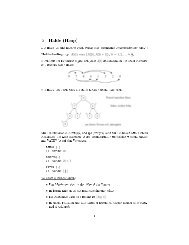
In this context, there is one geometric structure 

which is maybe most famous in computational 

geometry: Voronoi diagrams. Intuitively 

speaking, a Voronoi diagram divides the available 

space among a number of given locations (called 

sites), according to the nearest-neighbor rule: each 

site p gets assigned the region (of the plane, say) 

which is closest to p. A honeycomb-like structure 

is obtained; see Figure 1. 

Fig.1: Voronoi regions - aesthetically pleasing 

Christened after the Russian mathematician 

George Voronoi - believed to be the first to 

formally introduce it - this diagram has been 

reinvented and used in the past century in various 

different sciences. Area-specific names like 

Thema 

Wigner-Seitz zones (chemics, physics), domains 

of action (cristallography), Thiessen polygons 

(geography), and Blum’s transform (biology) 

document this remarkable fact. As of now, a good 

percentage of the computational geometry 

literature (about one out of 16 publications) is 

concerned with Voronoi diagrams. The 

computational geometry research group at Graz 

has been involved in this topic even before it 

became popular in the early 1980s (and long 

before our present institute has been founded). 

In this sense, research on Voronoi diagrams is a 

tradition at our place. For example, some 30 

publications by the second author, including two 

survey articles [4] [6] (the former also available 

in Japanese translation [5]) have emerged from 

this preference. 

We devote the present article to this fascinating 

geometric structure, with the intention to 

highlight its manifold role in computer science. 

Voronoi diagrams have proved to be a powerful 

tool in solving seemingly unrelated computational 

questions, and efficient and reasonably simple 

techniques have been developed for their 

computer construction and representation. 

Moreover, Voronoi diagrams have surprising 

mathematical properties and are related to many 

well-known geometric structures. Finally though, 

human intuition is guided by visual perception: 

if one sees an underlying structure, the whole 

situation may be understood at a higher level. 

Classical applications 

Voronoi diagrams capture the distance 

information inherent in a given configuration of 

sites in a compact manner. Basically, the structure 

is built from edges (portions of perpendicular 

bisectors between sites) and vertices (endpoints 

of edges). To represent a Voronoi diagram in a 

computer, any standard data structure for storing 

geometric graphs will do. Nonetheless, several 

tailor-made representations have been developed, 

7

Thema 

Fig.2: 3D view of sites and distances 

the most popular one being the quad-edge data 

structure. Simple graph-theoretical arguments 

show that there are at most 3n-6 edges and 2n-4 

vertices for n sites. In other words, the storage 

requirement is only O(n), which gives one more 

reason for the practical applicability of Voronoi 

diagrams. 

Continuing from our introductory example, 

imagine the given sites are post offices. Then, 

for any chosen location of a customer, the 

containing Voronoi region makes explicit the post 

office closest to him/her. More abstractly, by 

performing point location in the data structure 

‚Voronoi diagram‘, the nearest neighbor site of 

any query point can be retrieved quickly. (In 

fact, in O(log n) time. This is optimal by a 

matching information-theoretic bound). Similarly, 

sites may represent department stores, and 

Voronoi neighborhood - witnessed by diagram 

edges - will indicate stores in strongest mutual 

influence (or competition). Apart from 

economics, this basic finding has far-reaching 

applications in biological and physico-chemical 

systems. On the other 

hand, Voronoi vertices are 

places where the influence 

from sites reaches a local 

minimum - a fact of 

interest in facility location. 

Similar observations 

apply to the robotics 

scenery: sites are snapshots 

of moving robots, 

and danger of collision is 

most acute for the closest 

pair. Moreover, when 

planning a collision-free 

motion of a robot among a 

given set of obstacle sites, 

sticking to the boundaries 

of Voronoi regions (that is, 

moving along Voronoi 

edges and vertices) will 

keep the robot off the obstacles 

in a best possible 

way. (This is known as the 

retraction approach in 

motion planning.) 

Numerous other applications 

of Voronoi diagrams 

exist, one notable being 

geometric clustering. The 

grouping of data sites into 

a cluster structure is 

reflected by their Voronoi 

regions. (For instance, 

dense clusters give rise to 

regions of small area.) 

Even more important is the fact that prominent 

types of optimal clusterings are induced by 

Voronoi diagrams, namely by partition with 

regions (which are not necessarily defined by 

the data sites to be clustered). 

Two important and beautiful geometric structures 

cannot be hidden at this point. Firstly, any 

shortest connection network for the sites (think 

of a road or a electricity network) will solely 

connect sites which are Voronoi neighbors. 

Secondly, the graph connecting all the neighbored 

sites is a triangular network, called the Delaunay 

triangulation. Among all possible ways to build 

a triangular irregular network (TIN) the Delaunay 

triangulation is provably optimum, in several 

respects concerning the shape and size of its 

triangles (or tetrahedra, when it comes to higher 

dimensions). It is for this reason that Delaunay 

triangulations have been extensively used in 

surface generation, solid modeling, and related 

areas. 

Beside shortest connection networks (or 

minimum spanning trees, as they are called in 

computational geometry) there are several other 

classes of geometric neighborhood graphs which 

are contained in the Delaunay triangulation: 

α-shapes (a tool in surface modeling), β-skeletons 

(with applications to the famous and still 

unsettled minimum-weight-triangulation 

problem), Gabriel graphs (geographic information 

systems (GIS)), and nearest-neighborhood 

graphs (pattern recognition). 

Algorithms designer’s playground 

Methods for constructing Voronoi diagrams are 

as old as their use in the diverse areas of natural 

sciences. Of course, the first diagrams have been 

drawn with pencil and ruler. At these early times, 

people already complained about ambiguities if 

the sites come in a co-circular fashion. Nowadays, 

where sophisticated, efficient, and practical 

construction algorithms exist, robustness in the 

case of degenerate input sites is still an issue, 

and much of the program designers work goes 

into the implementation of ‚special cases‘. The 

heart of an algorithm, however, is the underlying 

paradigmatic technique, and rarely a problem has 

been better a playground for algorithms design 

than the computation of a Voronoi diagram. 

Beside other intuitive construction rules, 

incremental insertion has been among the first 

algorithmic techniques applied to Voronoi 

diagrams. This technique is well known from 

InsertionSort, a simple sorting method that 

maintains a sorted list during the insertion of 

items. In our case, insertion of a site means 

integrating its Voronoi region into the diagram 

constructed so far - a process that involves the 

construction of new and the deletion of old parts. 

Though the approach stands out by its simplicity 

and obvious correctness, the resulting runtime 

may be bad: finding a place to start the insertion 

is tricky, and many already constructed parts 

may have to be deleted lateron. It required the 

advent of randomization to give this approach 

an efficiency guarantee. To be more specific, 

inserting n sites in random order leads to an 

(expected) runtime of O(n log n) which is 

provably optimal. And only (almost-)optimal 

algorithms come up to a big advantage of the 

data structure Voronoi diagram: the linear storage 

requirement, O(n). 

„The intrinsic potential of Voronoi diagrams 

lies in their structural properties, in the existence 

of efficient algorithms for their construction, and 

in their adaptability.“ 

From: Handbook of 

Computational Geometry [5], 

Chapter V. 


Though the ancient Romans definitely knew 

about the power of „divide et impera“, its 

algorithmic analog divide & conquer is often 

considered a less intuitive technique. It achieves 

efficiency by splitting the problem at hands, then 

solving the subproblems separately (and 

recursively), and finally merging the solutions. 

Voronoi diagrams are well suited to this attack. 

After presorting the sites (in x-direction, say) 

the merging of two subdiagrams can be done in 

O(n) time, which calculates to a total runtime of 

O(n log n) by the recurrence relation 

T(n) = 2 ⋅ T(n/2) + O(n). Divide & conquer 

provided the first optimal algorithm for Voronoi 

diagrams, but certain peculiarities are buried in 

its implementation. On the other hand, it is a 

candidate for efficient parallelization. 

Two more optimal construction techniques are 

known, both being specific to geometry. The plane-sweep 

technique sweeps the plane containing 

the n input sites with a vertical line L, from left 

to right, say. Thereby, it maintains the invariant 

that all parts of the object to be constructed, 

which lie to the left of L, have already been 

completed. In this way, a 2D static problem (the 

construction of a Voronoi diagram) is translated 

into a 1D dynamic problem (the handling of the 

interactions near the sweep line). When utilizing 

the advanced data structures ‚priority queue‘ and 

‚dictionary‘, this event-driven algorithm runs in 

O(log n) time per event, the number of which is 

proportional to the size of a Voronoi diagram, 

O(n). 

Finally, geometric transformation is an elegant 

tool to gain algorithmic efficiency, via mapping a 

given problem to a better understood (and 

preferably solved) one. Its application to Voronoi 

diagrams is described in the next paragraph. 

Back to geometry 

Figure 2 gives a flavor of how proximity in 2D 

may be expressed by convexity in 3D. The 

surprising observation that a 2D Voronoi diagram 

is nothing but a projected convex 3D 

polyhedron opens our eyes - and a door to new 

construction methods. Polytope theory tells us 

to look for the geometric dual of that polyhedron 

(which now is the convex hull of n points in 3D), 

and indeed there is a simple rule to obtain these 

hull points directly from the given Voronoi sites: 

project them onto the paraboloid of rotation. 

The careful reader may notice that this very 

convex hull projects back to the afore-mentioned 

Delaunay triangulation of the sites in the plane. 

Convex hull algorithms are well established in 

computational geometry, and practical and 

robust implementations (running in time 

O(n log n) in 3D) are available. 


Noteworthy more is hidden in the geometric 

relation mentioned above. Firstly, the theory of 

convex polytopes allows us to exactly analyze 

the number of individual components of a Voronoi 

diagram. This is a highly non-trivial task in three 

and higher dimensions; faces of various 

dimensions (vertices, edges, facets, etc.) have to 

be counted in a thorough analysis of the storage 

requirement. Secondly, a connection to hyperplane 

arrangements is drawn, that is of importance 

when Voronoi diagrams are modified to 

order k. Here subsets of k sites get assigned their 

Voronoi regions; they carry the information for 

efficiently performing k-nearest neighbor search. 

Fig.3: Power diagram for 6 circles 

Finally, a natural generalization arises in the light 

of the geometric transformation shown in 

Figure 2. Power diagrams, defined by circular or 

spherical sites, and retaining the convexity of 

the regions. They constitute exactly those 

diagrams that are projected boundaries of convex 

polyhedra; Voronoi diagrams are special cases 

where circles degenerate to point sites. (When 

writing his doctoral thesis, the second author 

was excited when discovering the beauty and 

versatility of this structure; its name has been 

coined after one of his papers [3].) Power 

diagrams in 3D are related to important types of 

Voronoi diagrams in 2D, and thus provide a 

unified view of these structures. Among them 

are diagrams for sites with individual weights, 

expressing their capability to influence the 

neighborhood. These flexible models are used in 

other areas of science (Johnson-Mehl model in 

chemics and Appolonius model in economics). 

Even the mathematical physicist Clerk Maxwell 

in 1864 (implicitly) payed attention to power 

diagrams: he observed that a diagram reflects the 

equilibrium state of a spider web just if the diagram 

comes from projecting a polyhedron’s 

boundary... 

A novel concept 

In order to meet practical needs, Voronoi diagrams 

have been modified and generalized in many ways 

over the years. Concepts subject to change have 

been the shape of the sites (standard: points), 

the distance function used (standard: Euclidean 

metric), or even the underlying space (standard: 

the plane or 3-space). It is not appropriate here 

to give a systematic treatment of the various 

existing types of Voronoi diagrams. Instead, we 

would like to report on a particular type, which 

has been recently introduced and highlighted with 

success by our research group. 

Let us aid the reader’s intuition by giving a 

physical interpretation of Voronoi diagrams. 

Imagine a handful of small pebbles being thrown 

into a quiet pond, and watch the circular waves 

expanding. The places where waves interfere are 

equidistant from the pebbles’ hitting points. That 

is, a Voronoi diagram is produced. (This is the 

so-called growth model in biology and chemics.) 

Straight skeletons [1] are diagrams induced by 

wavefronts of more general shape. Consider a 

set, F, of simple polygons (called figures) in the 

plane. Each figure in F is associated with a birth 

time, and an individual speed for each of its edges 

to move in a self-parallel fashion. In this way, 

each figure sends out a polygonal wavefront 

(actually two, an external and an internal one). 

The straight skeleton of F now is the interference 

pattern of all these wavefronts, under the 

requirement that their expansion ceases at all 

points where wavefronts come into contact or 

self-contact. 

During their propagation, the wavefront edges 

trace out planar and connected Voronoi diagramlike 

regions. Wavefront vertices move at (speedweighted) 

angle bisectors for edges, and thus 

trace out straight line segments. We originally 

intended straight skeletons as a linearization of 

the medial axis, a widely used internal structure 

for polygons. (The medial axis is just the Voronoi 

diagram for the components of a polygon’s 

boundary. It contains parabolically curved edges 

if the polygon is non-convex.) In numerous 

applications, e.g., in pattern recognition, robotics, 

and GIS, skeletonal partitions of polygonal 

objects are sought that reflect shape in an 

Fig.4: Internal straight skeleton 

Thema 

9

Thema 

appropriate manner. The straight skeleton 

naturally suits these needs; see Figure 4. It is 

superior to the medial axis also because of its 

smaller size. 

Curiously enough, straight skeletons do not 

admit a distance-from-site definition, in general 

(and therefore are no Voronoi diagrams in the 

strict sense). This counter-intuitive finding 

outrules the well-developed machinery for 

constructing Voronoi diagrams; merely a 

simulation of the wavefront expansion will work. 

The theoretically most efficient implementation 

runs in roughly O(n √n) time, and a triangulationbased 

method that maintains ‚free-space‘ exhibits 

an O(n log n) observed behavior for many inputs. 

Straight skeletons apply to seemingly unrelated 

situations. This partially stems from a nice 3D 

interpretation, which visualizes the movement 

of each wavefront edge as a facet in 3D. The 

expansion speed of the edge determines the slope 

of the facet. In this way, each figure gives rise to 

a polyhedral cone in 3D, whose intersection with 

the plane is just the figure itself. The surface 

made up from these cones projects vertically to 

the straight skeleton. See Figure 5 for an 

illustration. 

A problem from architectural design is 

constructing a roof that rises above a given outline 

of a building’s groundwalls. This task is by no 

means trivial as roofs are highly ambigous objects. 

A more general question is the reconstruction of 

geographical terrains (say, from a given river map 

with additional information about elevation and 

slope of the terrain), which is a challenging 

problem in GIS. The straight skeleton offers a 

promising approach to both questions. Of 

particular elegance is the following property: the 

obtained 3D surfaces are characterized by the 

fact that every raindrop that hits the surface facet 

f runs off to the figure edge that defines f . This 

Fig.5: Terrain reconstructed from river map 

applies to the study of rain water fall and the 

prediction of floodings. 

Finally, there is an application to a classical 

question in origami design that deserves mention: 

is every simple polygon the silhouette of a flat 

origami? An affirmative answer has been found 

recently. The used method is based on covering 

certain polygonal rings that arise from shrinking 

the polygon in a straight skeleton manner. That 

is, our concept of straight skeleton allows for a 

relatively simple proof of this long-standing open 

conjecture in origami theory. 

...and the city Voronoi diagram 

Whereas the standard Voronoi diagram has 

interpretations in both the wavefront model and 

the distance-from-site model, this is not true for 

other types. Remember that straight skeletons 

cannot be defined in the latter model. Conversely, 

the occurance of disconnected Voronoi regions 

(as in the Apollonius model, where distances are 

weighted by multiplicative constants) disallows 

an interpretation in the former model. We conclude 

this article with a non-standard and demanding 

structure, that we have investigated recently, and 

that bridges the gap between both models. 

The structure in question - we called it the city 

Voronoi diagram [2] - is just the diagram matching 

the motivating example in the introduction. 

Recall that we are given a city transportation 

network that influences proximity in the plane. 

We model this network as a planar straight-line 

graph C with horizontal or vertical edges. No 

other requirements are posed on C - it may 

contain cycles and even may be disconnected. 

By assumption, we are free to enter C at any 

point. (This is not unrealistic for a bus system 

with densely arranged stops, and exactly meets 

the situation for shared taxis which regularly drive 

on predetermined routes and will stop for 

every customer.) Once having accessed C we 

travel at arbitrary but fixed speed v > 1 in one of 

the (at most four) available directions. Movement 

off the network takes place with unit speed, and 

with respect to the L 1 (Manhattan) metric. (Again, 

this is realistic when walking in a modern city). 

Let now d C (x, y) be the duration for the quickest 

route (which of course may use the network) 

between two given points x and y. When viewed 

as a distance function, this ‚city metric‘ d C 

induces a Voronoi diagram as follows. Each site s 

in a given point set S gets assigned the region 

{ x d ( x, 

s) 

< d ( x, 

t), 

∀t 

∈ S \ {} }. 

( s) 

= 

s 

reg C 

C 

Setting equality in this term gives the bisector of 

two sites s and t. This is the locus of all points 

which can be reached from s and t within the 

same (minimum) time. Bisectors are polygonal 

lines which, however, show undesirable 

properties in view of an algorithmic construction 

of the city Voronoi diagram. By C’s influence, 

they are of non-constant size, and even worse, 

they may be cyclic. These are main obstacles for 

efficiently applying divide & conquer and 

randomized incremental insertion. 

The key for a proper geometric and algorithmic 

understanding of the city Voronoi diagram lies in 

the concept of straight skeletons. Let us ignore 

the network C for a moment. The L 1 -metric 

Voronoi diagram for the sites in S already is a 

straight skeleton. Its figures are the L 1 unit circles 

(diamonds) centered at the sites. How does the 

network C influence their wavefronts? Their 

shapes change in a pre-determined manner, 

namely whenever a wavefront vertex runs into a 

network segment, or a wavefront edge slides into 

a network node. A new diamond will appear at 

such a place, along with tangent sharp-angled 

wedges whose peaks move at speed v in all 

possible directions on C. All these diamonds and 

wedges are taken as new figures. Together with 

the original L 1 diamonds, their straight skeleton 

now gives the city Voronoi diagram. 

Fig.6: A complex transportation network C (bold 

segments) and the city Voronoi diagram (full 

edges) for a set S of five sites scattered among C. 

The diagram is refined by straight skeleton edges 

(dashed). Quiet ranges occur in the network, 

shown as dotted subsegments. They could be 

closed down without delaying any quickest path 

to S. Also, one site is isolated from the network 

(the rightmost site s), in the sense that from 

nowhere in its region the quickest path to s takes 

advantage of C. 

In fact, the obtained skeleton contains a lot more 

edges (and information). Given a query point q, 

not only the first site s in S reachable from q can 

be retrieved, but rather the quickest route from q 

to s itself - a polygonal path of possibly high 

complexity. Still, this refined city Voronoi diagram 

has a size of only O(n+c), where n and c 

denote the complexity of S and C, respectively. 

(This important property is lost for non-isothetic 


networks or for the Euclidean metric; the size 

blows up to quadratic.) 

Two major difficulties have to be mastered before 

arriving at an efficient construction algorithm. 

Firstly the set of figures, when constructed from 

S and C as sketched above, contains high 

redundancy for various reasons. Secondly, when 

having available the set of O(n+c) non-redundant 

figures, a fast way of computing their straight 

skeleton has to be found. The second goal is 

achieved by modifying the figures so as to fit 

into the framework of so-called abstract Voronoi 

diagrams. 

This general and elegant framework extracts the 

desired algorithmic properties of a Voronoi diagram. 

It is based on an admissible system of 

bisectors, rather than on some distance from the 

sites. For example, for each triple of abstract 

sites, any point common to two bisectors must 

also belong to the third. (This property is trivially 

fulfilled for any distance-defined diagram, but is 

violated by straight skeletons, in general. ‚Noman‘s 

lands‘ belonging to no figure would arise 

from this ill-conditioning.) In our case, a careful 

adaption of the figures does allows a reduction 

to abstract Voronoi diagrams. The refined city 

Voronoi diagram then can be constructed in 

O(n log n + c 2 log c) time and optimal space. 

Fig.7: Direction-sensitive diagram [7]. Quo 

vadis? 

References 

This choice of references is highly selective. In 

particular, we refrained from listing all our 

publications relevant to Voronoi diagrams; this 

is done elsewhere in the present issue. 

[1] O.Aichholzer, F.Aurenhammer, Straight 

skeletons for general polygonal figures 

in the plane. In: Voronoi’s Impact on 

Modern Sciences II, A.M.Samoilenko 

(ed.), Proc. Institute of Mathematics of 

the National Academy of Sciences of 

Ukraine 21, Kiev, Ukraine, 1998, 7-21. 

[2] O.Aichholzer, F.Aurenhammer, B.Palop, 

Quickest paths, straight skeletons, and 

the city Voronoi diagram. Proc. 18 th Ann. 


ACM Symp. Computational Geometry 

2002. 

[3] F.Aurenhammer, Power diagrams: 

properties, algorithms, and applications. 

SIAM Journal on Computing, 16 (1987), 

78-96. 

[4] F.Aurenhammer, Voronoi diagrams - a 

survey of a fundamental geometric data 

structure. ACM Computing Surveys 23 

(1991), 345-405. 

[5] F.Aurenhammer. Voronoi diagrams - a 

survey of a fundamental geometric data 

structure (Japanese translation). BIT - 

ACM Computing Surveys ’91, Kyoritsu 

Shuppan Co., Ltd.(1993), 131-185. 

[6] F.Aurenhammer, R.Klein, Voronoi 

diagrams. Handbook of Computational 

Geometry, Chapter 5, J.Sack, G.Urrutia 

(eds.), Elsevier Science Publishing, 2000, 

201-290. 

[7] O.Aichholzer, F.Aurenhammer, D.Z.Chen, 

D.T.Lee, E.Papadopoulou, Skew Voronoi 

diagrams. Int’l. Journal of Computational 

Geometry & Applications 9 (1999), 235- 

247. 















Welcome to the 24th International 

Conference 

INFORMATION 

TECHNOLOGY 

INTERFACES 

Thema 

Collaboration and Interaction in 

Knowledge-Based Environments 

Cavtat / Dubrovnik, 

June 24-27, 2002 

ITI conference is organized by SRCE - 

University Computing Centre, University 

of Zagreb, with the aim to promote the 

interface of researchers involved in the 

development and application of methods 

and techniques within the broad 

framework of information and 

communication technology. ITI seeks 

papers that will advance the state of the 

art in the field and help foster increased 

interaction between academic and 

engineering communities. After 10 

successful conference years in the 3000 

years old city of Pula, Istria, ITI returns 

to a small, charming Adriatic town Cavtat 

near Dubrovnik! 

The Conference is sponsored by international 

association IMACS, co-sponsored 

by SCS and by WSES (World Scientific 

and Engineering Society), and supported 

by several foreign and Croatian academic 

institutions and societies, with English as 

the official conference language. 

11

Thema 

Points and Combinatorics 

Oswin Aichholzer * , Franz Aurenhammer, Hannes Krasser + 



Which point sets exist, anyway? 

This intuitive question sketches the topic of the 

article at hands. Its relevance is apparent: a 

configuration of n points is the underlying 

structure for countless problems in 

computational and combinatorial geometry. 

A point set is a (finite) collection of points in the 

plane, which are usually given by their x and y 

coordinates. In fact, point sets are among the 

simplest geometric objects that lead to non-trivial 

questions - in a geometrical, combinatorial, 

and algorithmic sense. Not surprisingly, most 

basic data structures in computational geometry 

have first been developed for point sets, and 

have been later generalized to more general 

objects, like line segments, circles, polygons, etc. 

Examples include geometric search trees, convex 

hulls, Voronoi diagrams (an accompaning article 

is devoted to this versatile structure), and many 

others. During the past two years, a good share 

of effort of our research group went into the 

systematic investigation of point sets of small 

size. Let us report on this original and challenging 

topic at this place. 

„There is a point in pointing out points, in order 

to order them by order type.“ 

The Realizing Enumerators O.F.&H. 

Of course, there exist infinitely many different 

sets of n points, for a given number n. However, 

quite a large class of problems is determined 

already by the combinatorial properties of an 

* Research supported by APART [Austrian Programme 

for Advanced Research and Technology 

of the Austrian Academy of Sciences] and the 

EU Improving Human Potential Programme 

HPRI-1999-CT-00071 

+ Research supported by the FWF [Austrian Fonds 

zur Förderung der Wissenschaftlichen Forschung] 

n-point set, rather than by its metric properties. 

⎛ n⎞ 

To be more specific, look at all the ⎜ ⎟ straight- 

⎝ 2⎠ 

line segments spanned by a given n-point set, as 

in Figure 1. Which of these line segments cross 

each other, and which don’t, turns out to be 

important: point sets with the same crossing 

properties give rise to equivalent geometric 

structures. This is valid for many popular 

structures, like spanning trees, triangulations, 

polygonalizations, so-called k-sets, and many 

more. 

Fig.1: Inequivalent sets of small size. There is 

only one (combinatorial) way to place 3 points, 

two ways to place 4 points, and three to place 5. 

The situation changes drastically for larger size. 

Several of these structures lead to notoriously 

hard problems. To gain insight, the study of 

typical (or extremal) instances is very fruitful. 

E.g., detecting a counter-example prevents 

us from constructing hopeless proofs. 

Conversely, the non-existence of counterexamples 

of small size gives some evidence for 

the truth of a conjecture. This motivates the 

complete enumeration of all problem instances 

of small size. In our case, this means investigating 

all inequivalent sets of points, where 

equivalence is with respect to their crossing 

properties. Let us ask again and more specifically, 

„Which inequivalent sets of, say 10, points do 

exist?“ 

The answer is surprisingly difficult, for two major 

reasons. Firstly, the number of inequivalent point 

sets of size 10 is already in the millions 

(14 309 547, to be precise). Secondly, there seems 

to be no simple way to enumerate all these sets. 

Each increase in set size gives rise to types which 

cannot be obtained directly from sets of smaller 

size. This may explain why it took until recently 

that an enumeration has been successful. We are 

proud to be the first having established (see [3]) 

and made available a complete and reliable data 

base 1 of all inequivalent 10-point sets (in 

December 2000). Meanwhile - in fact a few weeks 

ago - a further milestone was reached. We 

completed the generation of all inequivalent 

11-point sets (in implicit form). The present 

article describes the inherent difficulties of 

such a project, along with numerous applications 

and results we obtained from our point set data 

base. 

The theory behind 

Order types 

An appropriate tool to encode equivalence of 

point configurations has been developed by 

combinatorial geometers [15] quite a while ago. 

The order type of a set {p 1 , ..., p n } of points is a 

mapping that assigns to each (ordered) index 

triple i, j, k the orientation - clockwise or counterclockwise 

- of the point triple p i , p j , p k . (We 

require that no three points lie on a common 

straight line.) Two point sets S 1 and S 2 are 

considered equivalent if they exhibit the same 

order types. That is, there is a one-to-one 

correspondence between S 1 and S 2 such that each 

triple in S 1 agrees in orientation with the 

corresponding triple in S 2 . It is not hard to see 

that two line segments spanned by S 1 cross if 

1 http://www.igi.TUGraz.at/oaich/triangulations/ 

ordertypes.html 


and only if their counterparts in S 2 do so. Our 

aim is to enumerate all order types of given size 

n, for n ≤ 11. 

Duality 

We base our approach on a well-known duality 

between points and straight lines in the plane. 

By this duality, a set of points maps to a line 

arrangement, i.e., a dissection of the plane 

induced by a set of n straight lines. As no direct 

way to enumerate line arrangements is known, 

we first produce all (non-isomorphic) 

arrangements of so-called pseudolines. 

Pseudolines are simple curves that pairwise cross 

at exactly one point, just as non-parallel straight 

lines do. Handling pseudolines is relatively easy 

in view of their equivalent description by wiring 

diagrams; consult Figure 2. We can read off a 

corresponding pseudo order type from each wiring 

diagram: the order in which the wires cross each 

other determines the orientations for all index 

triples. Back in the primal setting, where each 

wire potentially corresponds to a point, this leads 

to a list of candidates guaranteed to contain all 

different order types. 

Realizability 

We are left with the problem of identifying all 

the realizable order types in the obtained list, 

that is, those for which corresponding point 

coordinates do exist. Here we enter the realm of 

oriented matroids, an axiomatic (combinatorial) 

abstraction of geometric objects, introduced in 

the late 1970s. As a known phenomenon, a wiring 

diagram need not be stretchable to straight. In 

fact, there exist non-stretchable diagrams already 2 

for 8 wires [10]. As a consequence, our candidate 

list will contain non-realizable pseudo order 

types for size n ≥ 9. Moreover, even if 

realizability has been recognized for a particular 

candidate, how can we find a corresponding point 

set? 

Fig.2: A wiring diagram that can be stretched 

Projectivity 

Surprisingly at first glance, the situation gets 

easier (conceptually and computationally) on the 

3D sphere, that is, in the projective setting. To 

2 Two of the authors won a pizza due to this 

peculiarity; the third was paying... 


visualize projective order types, imagine all 

possible ways n stars can be arranged in the sky. 

Watching stars from a fast moving space vessel 

changes their geometry, but not their projective 

order type. Unlike before, order types now 

directly correspond to arrangements of great 

circles by duality (and isomorphism classes of 

pseudo-circle arrangements coincide with 

reorientation classes of rank 3 oriented matroids). 

Moreover, the desired order types in the plane 

can be nicely grouped into projective classes, 

and in every class either each or no order type is 

realizable. 

Basic strategy 

In a nutshell, our approach works as follows. It 

produces a candidate list of planar pseudo order 

types (from wiring diagrams), clusters them into 

projective classes, and tries to decide realizability 

for each class. A collection of all yet unrealized 

projective classes is maintained. 

For problem sizes n = 9 and n = 10, the process 

could be terminated after the collection had 

shrunk to 1 and 242 members, respectively. We 

know from the literature that exactly that many 

classes are non-realizable [10, 14]. (The unique 

class for n = 9 derives from the well- known 

Tab.1: Numbers of different order types of size n 

Pappus theorem.) For the case n = 11, however, 

where information about projective classes is 

completely lacking, a means for disproving 

realizability had to be applied. 

Deciding realizability (for order types in 

particular and oriented matroids in general) is an 

intriguing problem, which is known to be NPhard. 

Several heuristics have been developed; see 

[14] and references therein. For our case, a singly 

exponential algorithm exists but turned out to be 

too slow, already for problem size 10. Instead, 

we used a combination of methods with success. 

Even for size 11, we could decide upon the status 

of all the projective classes, i.e., distinguish the 

realizables from the non-realizables. 

Coordinate recovering 

We applied an obvious though powerful insertion 

strategy in a first step: obtain realizations of size 

n from realizations of size n-1. Suppose that, for 

each (realizable) order type T of size 

n-1, a corresponding point set S(T) is available. 

Consider the arrangement A(T) formed by 

Thema 

⎛ n − 1⎞ 

⎜ ⎟ 

⎝ 2 ⎠ 

lines, each passing through a pair of points in 

S(T). Point sets of size n are now generated from 

S(T), by placing an additional point in a cell of 

A(T), for all possible cells. Carrying out this 

process for all existing order types of size n-1 

leads to realizations for a majority of order types 

of size n. 

However, the geometry of an (n-1)-point set S(T) 

critically affects the set of order types of size n 

which actually get realized. (This principal 

difficulty makes order type enumeration a hard 

problem.) To increase effectiveness, we restarted 

the insertion method after random (but order type 

preserving) perturbations of the (n-1)-point sets. 

All but a vanishing fraction of the realizable order 

types could be detected in this way, in fact, over 

99.99% even for n = 11. The rest (the ‚hard core‘ 

which contains the unrealizables, of course) we 

tried to realize directly - starting from scratch 

with tailor-made simulated annealing strategies. 

n 3 4 5 6 7 8 9 10 11 

Projectiv e Pseudo 

Order 

Types 

1 1 1 4 11 135 4 382 

312 356 

41 

848 

591 

- thereof 

non 

realizable 

1 242 155 

214 

= Projectiv 

e Order 

Types 

1 1 1 4 11 135 4 381 

312 114 

41 

693 

377 

Planar Pseudo 


Types 

1 2 3 16 135 3 315 

158830 14320182 2 343 

203 

071 

- thereof 

non 

realizable 

1310635 8 690 

164 

= Planar 


Types 

1 2 3 16 135 3 315 

158817 14309547 2 334 

512 

907 

Detecting non-realizability 

Clearly, certain pseudo order types notoriously 

denied themselves to realization. An obvious 

method to disprove their realizability is by 

detecting some non-realizable sub-order type as 

a witness. Though being powerful like the 

insertion strategy before (as being its reverse), 

the method has similar drawbacks: not all cases 

are covered. We therefore had to unmask certain 

non-realizables by different means. Following 

[10], we utilized the so-called Grassmann- 

Plücker relations, a determinant relation fulfilled 

by each 5-tuple of points in the plane. For a 

⎛ n ⎞ 

given pseudo order type of size n, these ⎜ . ⎟ 

⎝ 5 ⎠ 

relations lead to a linear program, whose 

infeasibility disproves its realizability. 

13

Thema 

„...one notices a peculiar asymmetry between the 

realizable and the non-realizable cases. There 

exists a simple and systematic representation for 

realizability proof, namely a sample point 

configuration. Even the longest and most 

complicated derivation of a realizability proof 

can be discarded once we have found some 

coordinate matrix. This means that we only need 

a few real algebraic numbers to finally encode 

the proof.“ 

From: Oriented matroids [10]. 

The data base 

Output 

Table 1 gives a quick overview of our results (in 

bold numbers), which significantly extend all relevant 

known results [14]. The tremendous 

growth of order types, especially in the planar 

case, becomes apparent. By the nature of our 

approach, we computed a combinatorial 

description for all the objects counted in Table 1, 

along with a geometric representation if the object 

is realizable. An obvious exception are the size- 

11 planar order types which - unless we are 

willing to spend some 160 CDs - have to be 

represented implicitly (by their projective 

classes). 

Size 10 

To get an impression of the computation time 

required, we give some details for the case n = 

10. The generation of all pseudo order types, 

plus partial realization using insertion, took 36 

hours on a 500 MHz Pentium III. Some 200 000 

pseudo order types were left unrealized. Most 

of the corresponding projective classes got some 

member realized, however, and could be 

completed quickly by applying a projection 

technique. Only 251 projective classes of 

undecided status remained. For these, we had to 

invoke our simulated annealing routines, as we 

had no information on which are the 242 classes 

known to be non-realizable. We were successful 

for 9 classes within 60 hours which completed 

this task. 

Size 11 

As expected, the situation turned out to be much 

more complex for n = 11. Although we further 

improved the implementation, the total time 

spent on projective classes was more than three 

months on several processors. Their planar 

members (which we are mainly interested in) 

can be derived on-line and independently for each 

particular class, and thus need not be stored. We 

point out once more that the time-consuming 

routines (simulated annealing and Grassmann- 

Plücker) were used only in ‚emergency cases‘ 

where the insertion technique (and its reverse) 

were no help any more. 

Whenever computing realizations, care was taken 

to avoid large coordinates. In addition, the simulated 

annealing routines were used to post-process 

the point sets. In their final form, our point sets 

enjoy several user-friendly properties, including 

a 16 bit integer representation. This should be 

contrasted with known negative results on the 

efficient grid embeddability of order types [16]. 

Reliability 

Despite the theoretical correctness of the 

algorithms used, the question arises of how 

reliable are our implementations. The wiring diagram 

based calculation of planar pseudo order 

types, including their grouping into projective 

classes, is of purely combinatorial nature. 

Evidence of correctness is gained from the 

correctly computed total numbers of projective 

pseudo order types for n ≤ 10 (which have been 

known before; see Table 1). 

The critical part are the geometric routines for 

both, proving and disproving realizability. As 

realizabilty is witnessed by the point sets (in 

nice representation), it can be re-checked in a 

reliable way. Non-realizability, on the other hand, 

may have no direct witness. We therefore put 

particular emphasis on the clean implementation 

of the geometric part of the Grassmann- Plücker 

routine, which basically is a linear program. 

Applicability 

In summary, a data base has been obtained that 

is complete, user-friendly, and reliable. Small integer 

coordinates ensure that all calculations based 

on our data base are efficient and numerically 

stable. Due to storage limitations, the point sets 

for sizes 10 and 11 are not accessible on-line, but 

rather have been stored on CDs which are 

available from us upon request. We believe our 

data base to be of value to many researchers who 

wish to examine their conjectures on small point 

configurations. 

The applicability of the data base is broad. In 

principle, any geometric straight-line structure 

is a candidate. Let us describe - for a few prominent 

questions - the progress achieved when 

using our data base. A more complete collection 

of our results is [5]. The concepts skipped here 

for space limitations include convex polygon 

covering, convex decomposition, pseudotriangulations, 

k-sets (partitioning lines), as well 

as the crossing-free variants of polygonalizations 

(Hamiltonian cycles), spanning trees, and 

matchings. 

Crossing numbers 

The (rectilinear) crossing number of a graph G 

is the least number of edge crossings attained by 

a straight-line drawing of G in the plane. To avoid 

trivialities, no three vertices of G may be collinear 

in the drawing. 

„...Our work was to bring out bricks from the 

ovens where they were made ...each oven was 

connected by rail with each store....trouble arose 

at the crossing of two rails. Here the cars jumped 

out, the bricks fell down; a lot of extra work and 

loss of time arose. Having this experience a 

number of times it occured to me why on earth 

did they build the rail system so uneconomically; 

minimizing the number of crossings the 

production could be made much more 

economical.“ 

From [18], Turan’s brick 

factory problem 

Fig.3: Minimal drawing of K 12 

It is easy to prove that drawings which differ in 

their numbers of crossings stem from vertex sets 

___ 

of different order types. Our interest is in cr( 

Kn 

) , 

the rectilinear crossing number of the complete 

graph K on n vertices. 

n ___ 

Determining cr( 

Kn 

) is commonly agreed to be a 

difficult task. From an algorithmic point of view, 

___ 

deciding whether cr( 

G) 

≤ k for a given graph G 

and parameter k, is NP-hard [9]. Despite the 

remarkable hunt for crossing numbers - initiated 

in [17] in the 1960s - only for very small n the 

___ 

exact values of cr( 

Kn 

) have been known, until 

recently. The instances n ≤ 9 have been settled 

quite a time ago, but no progress has been made 

until in 2001 two groups of researchers ([11] 

and the authors [3], respectively) independently 

___ 

found cr( 

K10) 

= 62. In [11] the goal was reached 

by a purely combinatorial argument, while our 

result came as a byproduct of the exhaustive 

enumeration of all order types of size 10. 

Encouraged by this achievement, we tailored our 

approach to generate inequivalent drawings of 


K for larger n. The effect was surprising. Not 

n 

only could we completely resolve the situation 

___ 

for n = 11 (to be precise, cr( 

K11) 

is 102, and this 

value is attained by exactly 374 inequivalent 

drawings), we also could break new ground for 

___ 

n = 12. More specifically, cr( 

K12) 

is 153, and the 

only known drawing that attains this value is 

Figure 3. These findings also implied the best 

known lower bound on the limit 

lim ___ 

cr n 

n→∞ 

which describes the ‚asymptotic gain‘ when 

drawing K optimally. In fact, this is a geometric 

n 

quantity of separate interest, by a connection to 

Sylvester’s four point problem [21]. For n ≥ 13, 

we constructed various new drawings of K with n 

few crossings, by insertion into the small optimal 

examples. These drawings led to improved 

upper bounds for the quantity above. The 

___ 

tantalizing question of determining cr( 

K13) 

is 

left open. By our calculations, the latest ra(n)ge 

is {221, 223, 225, 227, 229}; our conjecture is 

___ 

cr K ) = 229. 

( 13 

Compatible triangulations 

Can any two planar point sets (within the 

obvious size and convex hull restrictions) be 

triangulated in the same manner? Surprisingly, 

this basic question - which has applications in 

computer graphics (morphing) and in cartography 

(PLH maps) - is still unsettled. A triangulation 

of a set S of points is a maximal collection of 

non-crossing edges (line segments) spanned by 

S. Two point sets of the same order type allow 

for the same variety of triangulations. 

Triangulations are flexible constructs, which play 

a role in various areas and have important 

applications [8]; an obvious one is mesh 

generation. Their appealing structural properties 

won our interest right away. Beside Voronoi 

diagrams, triangulations have been the favorite 

structures of our research group; 15 publications 

arose in the last few years. Our work on this 

topic is partially reported in the survey article 

on optimal triangulations [7]. 

Returning to the question above, let S 1 and S 2 be 

two point sets in the plane. Two triangulations 

T 1 of S 1 and T 2 of S 2 are called compatible if there 

is a one-to-one correspondence ϕ: S 1 → S 2 with 

the following property: for each empty triangle 

ijk in T 1 , the points ϕ(i)ϕ(j)ϕ(k) define an empty 

triangle in T 2 ; see Figure 4. Compatible 

triangulations show isomorphic graphs of edges; 

the converse is not true, in general. 

The problem of triangulating two given point 

sets compatibly comes in two flavors, namely 

where the correspondence between their points 


⎛n 

⎞ 

( K ) / ⎜ ⎟ > 

⎝4 

⎠ 

0. 

311507 

is either fixed in advance, or variable. The case of 

fixed correspondence is a known problem. In 

particular, compatible triangulations do not 

always exist [19], because edges can be forced to 

cross (which is prohibited in a triangulation). 

The related decision problem is neither known 

to be NP-complete nor to be polynomially solvable. 

However, the problem becomes easier if 

the two point sets represent the vertices of two 

simple n-gons [6], namely decidable in O(n 2 ) time. 

We asked the different question, „under which 

conditions does there exist a correspondence 

which allows for compatible triangulations?“ 

Clearly, in both sets S 1 and S 2 the number n of 

points must be the same; as has to be the number 

h of extreme points (points on their convex hulls), 

by the well-known Eulerian formula e = 3n-h-3 

for the number of triangulation edges. 

Fig.4: These two triangulations are compatible 

Extreme points necessarily map to extreme 

points, and their cyclic order on the convex hulls 

is preserved. (More generally, for compatible 

triangulations any two corresponding triangles 

ijk and ϕ(i)ϕ(j)ϕ(k) must match in orientation. 

That is, their point sets locally exhibit the same 

order type.) Finally, both point sets have to be 

in general position, i.e., no three points on the 

same line are allowed. Counter-examples exist, 

otherwise; see Figure 5. 

Fig.5: No compatible triangulations exist 

These observations led us to state the following 

conjectures (which have been included in the 

recently founded open problems list in 

computational geometry 3 ). 

Main Conjecture 

Any two n-point sets that agree in the number 

of extreme points, and both are in general position, 

admit a compatible triangulation. 

3 http://www.cs.smith.edu/~orourke/TOPP/ 

node39.html#Problem.38 

Extended Conjecture 

The Main Conjecture still holds if a 

correspondence between the extreme points is 

prescibed (by a cyclically shifted labeling). 

The extended conjecture is relevant for a possible 

induction proof, which naturally will lead to 

assuming the stronger version as a hypothesis. 

In [2] we undertook first steps towards proving 

the conjectures. For instance, they are true if the 

number of interior points in either set is three or 

less. Obtaining an affirmative answer would be a 

deep theoretical result, showing that all planar 

point sets of the same size and hull size are 

‚topologically equivalent‘ in this very sense. The 

result, if true, gains in importance in view of the 

huge number of different order types for n points; 

cf. Table 1. 

In order to encourage and support future research 

on this topic, we are glad to announce the reward 

below. (A related playing tool 4 may turn out 

helpful.) 

ATTENTION - EuroPrizes! 

€ 30 for proving the Conjectures 

Thema 

+ an original Austrian Wiener Schnitzel 

€ 7 for a counter-example to the Main 

€ 5 for a counter-example to the Extended 

No reward for proving the Conjectures and 

providing a counter-example at the same time! 

Using our data base, we tested the Extended 

Conjecture for small point set sizes, and could 

verify it for up to 8 points. The lack of good 

heuristics for checking compatibility made the 

calculations time-consuming, however; they are 

still incomplete for size 9. Determining the 

theoretical complexity of computing compatible 

triangulations, if they exist, is an open problem. 

On the other hand, adding a small number of 

extraneous points (so-called Steiner points), 

which can be found efficiently, will always do 

the job [2]. 

Triangulation counting 

Efficiently counting all possible triangulations 

of a given n-point set (in general position) is an 

interesting open problem. To give a motivation, 

the question relates to computing random 

triangulations - a concept of importance for 

testing triangulation-based algorithms. 

The fastest counting method to date is based on 

a concept we called triangulation path [1]. Its 

running time still shows exponential growth, 

4 http://www.igi.TUgraz.at/oaich/triangulations/ 

compatible.html 

15

Thema 

however, and computations are limited to 

n ≤ 40. On the other hand, no good theoretical 

bounds on the number of triangulations are 

known. The current best maximizing examples 

yield 8 n-Θ(log n) triangulations, whereas the 

strongest upper bound is much larger, 59 n-Θ(log n) ; 

see [20]. 

Not even for small 

values of n, exact 

numbers have 

been known. But 

point sets of the 

same order type 

admit equally 

many triangulations, 

and so we 

could compute 

these numbers for 

n ≤ 10. Table 2 

lists their extremum 

values. The 

n minimu m maximum 

3 1 1 

4 1 2 

5 2 5 

6 4 14 

7 11 42 

8 30 150 

9 89 780 

10250 4550 

Tab.2: Extremum numbers 

of triangulations 

currently best examples for n = 11 through 20 

can be found on-line 5 . 

Fig.6: Double-circle configuration 

So, for example, every set of 8 points must have 

at least 30 triangulations, and there actually exists 

a set having that few triangulations. This shows 

that point sets in convex position, whose number 

of triangulations is given by the so-called Catalan 

numbers C(n-2) (yielding 132 for n = 8), do not 

lead to the minimum. This conjecture would 

have been plausible, as it is true for other 

structures, namely for crossing-free matchings 

and crossing-free spanning trees [13]. Though 

the conjecture has been resolved before, the 

results in Table 2 may be useful in proving or 

disproving the extremal behavior of other point 

configurations. For instance, we could observe 

that the point sets leading to the lower bounds in 

Table 2 obey a rather special structure. We 

conjecture that these ‚double-circle‘ 

5 http://www.igi.tugraz.at/oaich/triangulations/ 

counting/counting.html 

configurations - shown in Figure 6 - indeed yield 

the minimum for general n. 

A legitimate question is, „How many 

triangulations must every n-point set have?“ 

Surprisingly little is known in this respect. We 

therefore seek for functions t(n) such that every 

set of n points exhibits Ω(t(n)) triangulations. A 

quick answer is t(n) = 2 (n-4)/6 , because every 

triangulation on n points contains at least 

(n-4)/6 edges that can be flipped (i.e., replaced 

by a crossing edge within the same quadrilateral) 

in an independent way [12]. A substantial 

improvement is based, among other things, on a 

new result on crossing families (pairwise crossing 

edges), which we found out by checking order 

types: every set of 10 points already spans a 

crossing family of size 3. (This drastically 

improves on the previous best bound of 37, in 

[22].) 

We exploited this result [4] to obtain the relation 

t n) 

≥ 3⋅ 

t( 

n ) ⋅t( 

n ) 

( 1 2 

for n 1 +n 2 = n+2. For any base α, the function 

t(n) = 1/3 ⋅ α n-2 is a solution. To get the recurrence 

started, values of α as large as possible are sought 

by examining all instances of small constant size. 

This is done by utilizing Table 2, in combination 

with other methods. The best value we achieved 

is α = 2+ε for ε < 1/80, that is, 

1 

n 

t( n) 

> ⋅ ( 2 + ε ) . 

13 

This constitutes the first bound that 

asymptotically beats the magic threshold 2 n . 

The enumeration of combinatorial objects clearly 

is limited to small object size. Still, proving a 

general property may boil down to a case analysis 

of constant-size problems. Proofs that require a 

non-trivial induction base are an example . . .The 

point is that the quality of the induction base affects 

the asymptotics of the result. In this way, 

‚constant‘ knowledge may well lead to insight 

concerning ‚infinity and beyond‘... 

References 

[1] O.Aichholzer, The path of a triangulation. 

Proc. 15th Ann. ACM Symp. on 

Computational Geometry, 1999, 14-23. 

[2] O.Aichholzer, F.Aurenhammer, F.Hurtado, 

H.Krasser, Towards compatible 

triangulations. Theoretical Computer 

Science (invited). 

[3] O.Aichholzer, F.Aurenhammer, H.Krasser, 

Enumerating order types for small point 

sets with applications. Proc. 17th Ann. 

ACM Symp. on Computational 

Geometry, 2001, 11-18. 

[4] O.Aichholzer, F.Hurtado, M.Noy, On the 

number of triangulations every planar 

point set must have. Proc. 13th Ann. 

Canadian Conf. on Computational 

Geometry, 2001, 13-16. 

[5] O.Aichholzer, H.Krasser, The point set 

order type data base: a collection of 

applications and results. Proc. 13th Ann. 

Canadian Conf. on Computational 

Geometry, 2001,17-20. 

[6] B.Aronov, R.Seidel, D.Souvaine, On 

compatible triangulations of simple 

polygons. Computational Geometry: 

Theory and Applications 3 (1993), 27- 

35. 

[7] F.Aurenhammer, Y.-F.Xu, Optimal 

triangulations. In: Encyclopedia of 

Optimization 4, P.M.Pardalos and 

C.A.Floudas (eds), Kluwer Academic 

Publishing, 2001, 160-166. 

[8] M.Bern, D.Eppstein, Mesh generation and 

optimal triangulation. In: D.-Z.Du, 

F.K.Hwang (eds.), Computing in 

Euclidean Geometry, Lecture Notes 

Series in Computing 4, World Scientific, 

Singapore, 1995, 47-123. 

[9] D.Bienstock, Some provably hard crossing 

number problems. Discrete & Computational 

Geometry 6 (1991), 443-459. 

[10] A.Björner, M.Las Vergnas, B.Sturmfels, 

N.White, G.Ziegler, Oriented Matroids. 

Cambridge University Press, 1993. 

[11] A.Brodsky, S.Durocher, E.Gether, The 

rectilinear crossing number of K 10 is 62. 

The Electronic J. of Combinatorics 8 

(2001), Research Paper 23. 

[12] J.Galtier, F.Hurtado, M.Noy, S.Perennes, 

J.Urrutia, Simultaneous edge flipping in 

triangulations. Manuscript, Universitat 

Politecnica de Catalunya, Barcelona, 

Spain, 2000. 

[13] A.García, M.Noy, J.Tejel, Lower bounds 

on the number of crossing free subgraphs 

of K n , Computational Geometry: Theory 

and Applications 16 (2000), 211-221. 

[14] J.E.Goodman, Pseudoline arrangements. In 

J.E.Goodman, J.O’Rourke (eds.), 

Handbook of Discrete and Computational 

Geometry. CRC Press LLC, Boca 

Raton, NY, 1997. 

[15] J.E.Goodman, R.Pollack, Multidimensional 

sorting. SIAM J. Computing 

12 (1983), 484-507. 

[16] J.E.Goodman, R.Pollack, B.Sturmfels, 

Coordinate representation of order types 

requires exponential storage. Proc. 21st 

Ann. ACM Sympos. Theory of 

Computing, 1989, 405-410. 


[17] R.K.Guy, A combinatorial problem. Nabla 

(Bulletin of the Malayan Mathematical 

Society) 7 (1960), 68-72. 

[18] R.K.Guy, The decline and fall of 

Zarankiewicz’s theorem. In: Proof 

Techniques in Graph Theory (Proc. 2nd 

Ann Arbor Graph Theory Conf.), 63- 

69, Academic Press, New York, 1969. 

[19] A.Saalfeld, Joint triangulations and 

triangulation maps. Proc. 3rd Ann. ACM 

Sympos. Computational Geometry, 

1987, 195-204. 

[20] F.Santos, R.Seidel, On the number of 

triangulations. Manuscript, Universität 

des Saarlandes, Saarbrücken, Germany, 

2000. 

[21] E.R.Scheinerman, H.S.Wilf, The rectilinear 

crossing number of a complete graph and 

Sylvester’s „four point problem“ of 

geometric probability. Amer. Math. 

Monthly 101 (1994), 939-943. 

[22] G.Tóth, P.Valtr, Note on Erdös-Szekeres 

theorem. Discrete & Computational 

Geometry 19 (1998), 457-459. 















Dipl. Ing. Hannes Krasser, computer scientist 

and mathematician, Ph.D. student of Prof. Franz 

Aurenhammer at the Institut für Grundlagen der 


Homepage: http://www.igi.tugraz.at/hkrasser 


IEEE IEEE IEEE Inter Interna Inter Inter na national national 

tional Conf Confer Conf Confer 

er erence er ence on 

on 

Multimedia Multimedia and and Expo 

Expo 


August 26-29, 2002 

Lausanne, Switzerland 

Thema 

17

Thema 

Sorting it out: Machine Learning and 

Fingerprints 

Anton Schwaighofer 

Siemens Corporate Technology, München, and Institut für Grundlagen 

der Informationsverarbeitung, Technische Universität Graz 

Abstract 

Machine learning concepts can find applications 

in many domains. We describe here one such 

application to the problem of fingerprint 

verification. In biometric verification using 

fingerprints, one often has to handle large archives 

of fingerprint images. When verifying an individual 

fingerprint, it is important to have a fast 

method at hand that selects suitable candidate 

images out of a large archive. We present an 

approach to sort a fingerprint archive according 

to similarity with a given fingerprint, inspired 

by an opto-electronic device called the wedgering-detector. 

The goal 

With the advent of electronic banking, electronic 

commerce and smart-cards, more and more personal 

data - such as credit card numbers or medical 

records - is stored electronically. Reliable systems 

for automatic personal identification are becoming 

increasingly important. Fingerprints have 

become popular as a means of personal 

identification, since relatively cheap sensors are 

available. State-of-the-art fingerprint sensors 

occupy an area of a postage stamp and are less 

than 1 mm thick. 

The framework for the work presented here is 

the Siemens ID Mouse, a computer mouse with 

an integrated fingerprint sensor. The main 

application area of the ID Mouse is access 

control to a PC. The user no longer has to enter 

his or her password to gain access, but simply 

puts a finger onto the fingerprint sensor. 

When using the ID Mouse in large scale 

applications such as network-wide identification, 

methods to efficiently handle large archives of 

fingerprints become necessary. Using concepts 

developed in machine learning, we first devise a 

compact representation of fingerprint images, 

based on spectral features of the images. In a 

second step, a similarity function based on the 

chosen representation is tailored specifically to 

comparing fingerprint images. In combination, 

this gives an efficient and accurate method of 

sorting a large archive of fingerprints according 

to coarse level similarity with a given request 

fingerprint. 

Fig.1: An example fingerprint image. Classical 

fingerprint verification is based on the so-called 

minutiae, the end points and bifurcations of the 

finger ridges (marked by circles). When a 

sufficient number of minutiae in two fingerprints 

agree in both type and orientation, the fingerprints 

are assumed to be identical. 

Classical fingerprint 

recognition 

Fingerprints are among the 

earliest and best-known 

biometric identification 

methods. Developed primarily 

for the identification of 

criminals, the use of 

fingerprints has been extended 

to, for example, amnesia 

victims or unknown deceased. 

Basis of classical fingerprint 

recognition techniques are the 

end points and bifurcations of 

the finger ridges, the so-called 

minutiae. A sample fingerprint 

image with marked minutiae is 

shown in Figure 1. 

Fingerprint recognition systems based on 

minutiae consist loosely speaking of three stages: 

Image pre-processing, locating the minutiae, and 

comparing the minutiae list of both fingerprints, 

often solved as a constrained graph matching 

problem. Easy as this may sound at the first 

glance, this process has many stumbling blocks. 

Each of the processing steps requires careful finetuning 

of parameters and handling of ambiguous 

cases. Thus, the whole process of comparing 

two fingerprints may become rather timeconsuming. 

Spectral features of fingerprints 

For our purposes, we wish to have a 

representation of fingerprint images that captures 

global image properties. Using such global 

features, fingerprints can be compared at a coarse 

global level first, and only at a second stage the 

local features (minutiae) will be used. 

Due to the inherent periodic structure of a 

fingerprint, ridge frequency and ridge orientation 

seem to be a good choice. It is well known that 

the Fourier transformation of an image can 

F( 

u, 

v) 

⎞ 

⎟ 

M ⎟ 

⎟ 

F( 

u, 

v) 

⎟ 

⎠ 

18 Telematik 1/2002 

⎛ 

⎜ 

r = ⎜ 

⎜ 

⎝ 

∑ 

∑ 

u, 

v∈A 

u, 

v∈H 

Fourier transform F (u; v) 

Original Image I(x,y) ⇒ ⇒ of the image, plus ⇒ ⇒ Output vector r 

boundaries of the WRD regions. 

Fig.2: The wedge-ring-detector (WRD) is applied to an image. The 

detector has 4 wedge-shaped regions A...D and 4 ring-shaped regions 

E...H. Integrating (resp. summing) the spectral energy of each region 

gives a feature vector r that is used as the representation for the 

fingerprint image I(x; y). This drawing is schematic, the wedge-ringdetector 

that is effectively being used has 12 rings and 8 wedges.

capture such global features. When browsing 

through the literature, we came across a device 

inspired from opto-electronics, called the wedgering-detector 

(WRD). The idea of the WRD is as 

follows: 

1. Compute the discrete Fourier transform of 

the image. 

2. Partition the Fourier transform into wedgeshaped 

and ring-shaped regions. These 

regions correspond to different ranges and 

orientations of spatial frequency. 

3. Integrating the Fourier transform over each 

of these regions gives a figure describing the 

amount of spectral energy in the 

corresponding region. 

The whole process of applying the WRD to a 

fingerprint image is summarized in Figure 2. By 

checking the properties of the Fourier transform, 

we recognize that the features from integrating 

over rings are (to a certain extent) invariant under 

rotation. All features are (again only to a certain 

extent) invariant under translation, since the 

WRD integrates over absolute values. The 

wedge-ringdetector thus provides us with a 

single vector describing global and invariant 

properties of the fingerprint image. 

Feature optimization 

Above we have described the process of 

computing a global description of a fingerprint 

image by means of the so-called wedge-ringdetector 

(WRD). This method has been used for 

long in opto-electronics and also in some previous 

work on finger-print recognition [3]. 

Fig.3: The principle behind the Bhattacharrya 

bound. The plot shows the distribution of feature 

values for points from classes C1 and C2 . For 

both classes, the feature value has Gaussian 

distribution. We might now try to assign points to 

the classes C1 and C2 by setting a simple 

threshold ω. But since the two classes have a 

region of overlap, this classification will not be 

error free - no matter how sophisticated the 

classification scheme is. The error is proportional 

to the area marked gray in the plot. The 

Bhattacharrya bound gives a lower bound on 

the error, computed from mean and variance of 

the class distributions. 


At this point, machine learning (ML) finally 

comes into play. We use ideas from ML to 

improve on two distinct points: 

1. We use a statistical criterion to optimize the 

position and size of wedges and rings, that 

is, the parameters of the WRD. It turns out 

that we can gain a lot of discriminative power 

by tailoring the WRD specifically to 

fingerprint images. 

2. In a simple system, we might want to 

compare two fingerprint images only on the 

basis of their WRD feature vectors, leaving 

aside any other information such as minutiae. 

Using adaptive techniques, namely neural 

networks and support vector machines, we 

can learn a function that takes two WRD 

feature vector as input and computes the 

degree of similarity of the two corresponding 

fingerprint images. 

To optimize the arrangement of wedges and rings 

in the WRD, we employ the so-called 

Bhattacharrya-bound [1]. Figure 3 briefly 

illustrates this concept. The basic idea of our 

optimization procedure is to look at pairs of 

fingerprint images, each fingerprint being 

represented by its WRD feature vector. Each 

pair either shows the same finger (call that class 

C 1 ) or two different fingers (class C 2 ). We assume 

that both classes have a Gaussian distribution. 

These two classes will not be separable perfectly, 

due to ambiguities in the images and mostly due 

to the simple representation via the WRD feature 

vector. This means that no method, no matter 

how sophisticated it is, can tell precisely whether 

the two fingerprint images show the same finger 

or not. The error of a (hypothetical) optimal 

method is bounded from below by the 

Bhattacharrya distance of the classes C 1 and C 2 . 

Our idea to find the optimal arrangement of rings 

and wedges in the WRD (the WRD parameters) 

is to minimize the Bhattacharrya distance. We 

choose the parameters such that the fingerprint 

representation allows a classification with 

minimum error. We proceed as follows: We 

iteratively modify one parameter, keeping all 

others fixed. With the current parameter setting, 

all feature vectors for a given set of fingerprint 

images are computed. We set the parameter to 

that value which minimizes the Bhattacharrya 

distance. We so found optimized values for the 

following parameters of the WRD: 

� radius of the innermost and outermost ring 

� inner and outer radius of the wedges 

� number of rings and number of wedges 

Thema 

In existing literature, the WRD is always used in 

a non-optimized way. On a test set of 407 

fingerprint images, the use of an optimized WRD 

with 20 rings and wedges lead to a reduction of 

error rates by 20%, when compared to the same 

setting with a non-optimized WRD (Table 2 lists 

the detailed results). Even higher improvements 

through the use of the optimized WRD will be 

shown in the last section. 

An adaptive similarity function 

In the previous section we have shown a method 

of representing a fingerprint image by a 

lowdimensional vector, computed with the 

wedge-ring-detector. Based on this 

representation we can now answer the question 

which fingerprint image in an archive (reference 

fingerprints) matches a given request fingerprint. 

We might do so by computing the Euclidean 

distance between feature vectors and select that 

reference fingerprint that has the lowest Euclidean 

distance. Such a simplistic approach will of 

course not be sufficiently accurate for practical 

use, yet it will become a very helpful tool in the 

next section. 

It turned out that this simple strategy can be 

improved by means of an adaptive similarity 

function that replaces the Euclidean distance. We 

obtain the similarity function by using a learning 

algorithm. A learning algorithm as we use it here 

can be looked upon as a family of parameterized 

functions. Training points consist of function 

input value and desired output value. During 

training, the parameters of the learning algorithm 

are chosen to minimize an error criterion, 

evaluated on the training points. Output of the 

training stage is a function with optimally chosen 

parameters. 

The training data for our task here are generated 

from a set of fingerprint images from 43 fingers, 

with 4 different images per finger. We consider 

each pair of fingerprint images, both represented 

by their wedge-ring-detector feature vector. If 

both images show the same finger, we set the 

corresponding target value to 1, otherwise to 0. 

It turned out that the best learning algorithm for 

this kind of problem was the Support Vector 

Machine (SVM, see for example [2]), a linear 

classifier that has been used with great success 

for problems ranging from handwritten digit 

recognition to text classification. Input to the 

SVM are two feature vectors representing 

fingerprint images, the SVM outputs the degree 

of similarity between the two images. Table 1 

shows that the use of the SVM can improve the 

error rates of the above mentioned simplistic 

fingerprint recognition system by another 10%. 

19

Thema 

Overall system performance 

Comparing two fingerprint images in detail is a 

very time-consuming task. When using a minutiae 

based approach (see Fig.1) the comparison boils 

down to comparing two minutiae lists. Minutiae 

in both images should agree in type (bifurcation 

or end point), orientation and distance to other 

minutiae. Since we have to account for rotation, 

translation, missing and false minutiae as well, 

this may become a lengthy procedure. This is 

not so much a problem as long as the number of 

reference fingerprints is small (say, 10). Once 

the number reaches 100 or even millions in large 

fingerprint databases, a simple matching strategy 

such as comparing the request fingerprint with 

all reference fingerprints is clearly unpractical. 

MethodErrorrateontestset Non-optim 

ized 

wedge-rin 

g-detector, 

compare 

feature 

vectors 

via 

Euclid 

ean 

distance 

( as 

used 

in 

literatu 

re) 

Optimiz 

ed 

wedge-rin 

g-detector, 

compare 

via 

Euclid 

ean 

distance 

Optimiz 

ed 

wedge-rin 

g-detector, 

compare 

via 

Support 

Vector 

Machine 

14, 

7 

The whole process of fingerprint matching is 

thus being split up into two parts: 

1. The pre-matcher selects those images from 

the archive of reference images that are most 

similar to the given request fingerprint. These 

images are called the candidate images. A 

suitable measure of similarity has to be defined. 

2. The matcher takes the list of candidate 

fingerprints and performs a detailed 

comparison of the request fingerprint with 

all candidate fingerprints. If no matching 

fingerprint can be found in the candidate set, 

we assume that the request fingerprint does 

not match any of the reference images. 

Based on the ideas presented in the previous 

sections, we propose the following pre-matcher. 

We first compute the wedge-ring-detector feature 

vector for the request image. Then scan over the 

whole archive of reference fingerprints and feed 

the WRD feature vectors of each reference 

fingerprint and request fingerprint into the ad- 

% 

13, 

04 

% 

11, 

68 

% 

Tab.1: Performance of a simplistic fingerprint 

recognition system. One can observe the reduction 

of error rates that is achieved by first optimizing 

the WRD specifically for fingerprint images, and 

secondly by using an adaptive function (SVM) to 

compare the feature vectors. The error rates are 

of course far too high to be used in a stand-alone 

system, yet they provide a good basis for use as 

a pre-matching system (see text) 

aptive similarity function. The pre-matcher 

selects now as the candidate set those reference 

images that show the highest degree of similarity 

to the request image. Since the reference feature 

vectors can be computed in advance, the prematcher 

can be run at low computational cost. 

The identification system in the ID Mouse 

software has already been equipped with a 

prematcher, yet based on a different idea. We 

now compare the performance of our proposed 

pre-matcher to the performance of the currently 

used pre-matcher, using the following criteria: 

� Overall error rate of the system (pre-matcher 

and matcher). 

� Average position of the matching fingerprint 

in the candidate set (winner average position 

WAP). An ideal pre-matcher would place the 

one reference image that matches the request 

at the first position in the candidate set, 

whereas a worst-case pre-matcher would not 

place the matching reference image into the 

candidate set. Low WAP will lead to a low 

overall runtime. 

Criterio 

n 

Improveme 

nt 

over 

existin 

g pre-matche 

r 

Testset1Testset2 E rror 

rate, 

medium 

security 

setting 

2 5 % 31 

% 

E rror 

rate, 

high 

security 

setting 

6 7 % 38 

% 

Winne 

r average 

position, 

medium 

security 

setting 

4 5 % 50 

% 

Tab.2: Performance improvement of a fingerprint 

recognition system with wedge-ring-detector prematcher 

(WRD, as proposed in this article) over 

the currently used pre-matcher. In all cases, the 

WRD pre-matcher lead to a drastical 

improvement of error rates. Furthermore, the 

winner average position reduced by around 50% 

and thus halved the overall runtime, since 50% 

fewer reference images need to be compared in 

detail by the matcher. 

Results on two distinct test sets (with 950 and 

1400 fingerprint images) are listed in Table 2. 

The quality of the proposed pre-matcher shows 

up clearly from the strikingly high reduction of 

error rates. In particular, the reduction of error 

rates in the high security is remarkable. This high 

reduction may be explained from the fact that 

matcher and pre-matcher use independent image 

features (minutiae vs. spectral energy) and so 

provide two complementary „views“ of the 

fingerprint. In particular in a high security setting, 

matching two complementary views will clearly 

increase confidence and reduce error rates. 

Conclusions 

For use in the fingerprint recognition software 

of the Siemens ID Mouse, we have devised and 

investigated a simple way of comparing two 

fingerprint images, based on features derived from 

the Fourier transform of the image. Details on 

methodology and an exhaustive list of results 

can be found in [3]. 

Using some concepts developed in machine 

learning, we were able to find a low-dimensional 

representation of fingerprint images that allows 

an accurate coarse-level comparison of two 

fingerprints. While not being sufficiently accurate 

as a stand-alone system, this coarse comparison 

turned out to be highly successful as a means of 

sorting large archives of fingerprints. 

Particularly impressive results were obtained 

when this sorting method was used as the prematcher 

for a traditional fingerprint matcher. On 

basis of the spectral representation, the prematcher 

selects out of a large archive those 

fingerprints that are similar to a given request 

fingerprint. The most similar ones are compared 

to the request image in detail, using a traditional 

fingerprint matching method. We were able to 

improve overall error rates by approx. 30% 

(depending on the test data set) and reduce the 

number of required detailed matching operations 

by 50%. Due to the large performance 

improvements, the proposed pre-matcher has 

been fully integrated into the ID Mouse software. 

Acknowledgements 

This work was done while the author was at 

Siemens PSE PRO SRT Graz. Fruitful 

discussions with Kurt Heschgl, Wolfgang Marius, 

Ernst Haselsteiner, Bernd Wachmann, Josef 

Birchbauer and Ulrich Haage, as well as the 

support from Wolfgang Maass and Gerd 

Hribernig, are greatfully acknowledged. 

References 

[1] K. Fukunaga. Introduction to Statistical 

Pattern Recognition. Academic Press, 

San Diego, CA, 2 nd edition, 1990. 

[2] B. Schölkopf and A.J. Smola. Learning with 

Kernels. MIT Press, 2002. 

[3] A. Schwaighofer. Fingerprint matching with 

spectral features. Master’s thesis, Institute 

for Theoretical Computer Science, 

Graz University of Technology, Austria, 

May 2000. 

Dipl. Ing. Anton Schwaighofer, computer 

scientist, studied Telematik at the TU Graz, 

currently Ph.D.-student of Prof. W. Maass at 

Siemens Corporate Technology in München. 

Homepage: http://www.igi.tugraz.at/aschwaig 


Why Students Don’t Ask Questions 

Peter Auer 



Abstract 

We analyse the number of questions which a 

rational student will ask in a learning situation, 

depending on his or her objective. For this we 

propose a formal learning model and two 

possible objectives of the student. In this learning 

model material is presented to the student in 

small bits, the student may ask arbitrary yes-no 

questions about the material, and occasionally 

the teacher will query the student to access his 

understanding of the material. 

In the first scenario that we will consider, 

questions asked by the student are regarded as 

faults. The objective of the student is to minimize 

the number of questions that he asks plus the 

number of incorrect answers that he gives to the 

teacher’s queries. The result of our analysis is 

that in such a scenario a student will ask rather 

few questions. 

In the second scenario the student’s objective is 

to minimize the number of incorrectly answered 

queries and to be efficient with her learning time. 

We will argue that there are cases in which a 

student who asks no questions will need much 

more time to learn than a student who asks 

questions. 

Introduction 

This account on student strategies is an attempt 

to put results from computational learning theory 

into a framework which is well known to many 

of us. In this paper we address a fundamental 

question: How much better does an active learner 

acquire information compared to a passive learner. 

In our model an active learner might ask arbitrary 

yes-no questions about the material to be learned, 

whereas a passive learner never asks questions 

but passively follows the material presented by 

the teacher. The somewhat surprising result is 

that an active learner acquires information not 

much more efficient than a passive learner. 

To measure information acquisition we count the 


number of times the student has to change his 

concept of the taught material. Fewer changes of 

concept - until the learned concept is correct - 

indicate a more efficient acquisition of 

information. We will show that a passive learner 

needs to change his concept at most 2.5 times 

more often than an active learner. 

The picture gets very different if we measure the 

amount of computation needed by active and 

passive learners 1 . We will provide evidence that 

in some cases the amount of computation of an 

active learner might be much smaller than the 

amount of computation of any passive learner. 

In the following section we define our model 

more precisely and state the relevant results and 

consequences for student strategies. Then these 

results are derived for the information oriented 

view on learning and for the computation oriented 

view. 

The learning model 

What to learn 

We are interested in a model where a teacher 

presents some material to a student in an 

incremental way. We represent such material as 

a bit sequence y = 〈y 1 , . . ., y T 〉, y t ∈{0, 1}, 1 ≤ t 

≤ T, of length T . At each step t the teacher gives 

bit y t to the student. Before giving y t to the 

student the teacher might decide to query the 

student about y t . In this case the student has to 

predict the true y t by some yˆ t ∈ {0, 1}. If yˆ t ≠ 

y t then the student’s prediction was a mistake. 

We assume that the bit sequence y is not 

completely arbitrary but that it has some 

structure. As an example y might be a textbook 

where expository chapters are followed by 

exercises and the student is queried only about 

the solutions of the exercises. We denote by Y 

1 Essentially we are measuring the „thinking 

time“ of the learners. 

Thema 

the class of all bit sequences with the relevant 

structure. The student knows about the structure 

of the taught material, i.e. she knows that y ∈ Y . 

Active and passive learners 

We will distinguish between active and passive 

learners. An active learner may ask arbitrary yesno 

questions about y at any time. These questions 

are answered correctly by the teacher. Formally 

each yes-no question about a property of y can 

be formulated as „Is y ∈ Y´ ?“ where Y´ ⊆ Y is the 

subset of all sequences in Y with the respective 

property. A passive learner never asks a question. 

Remark: In computational learning theory several 

similar models are investigated. The maybe most 

general model in this context considers sequences 

of input/output pairs (x, y) = 〈(x 1 , y 1 ), . . ., (x T , 

y T )〉 where x t ∈ X and y t ∈ Y for some input 

domain X and some output domain Y. [2] 

Information complexity of learning 

As mentioned in the introduction we want to 

measure the information complexity of a learning 

task by the number of times the learner changes 

its concept of the taught material y. Why does 

this make sense? Because this is the amount of 

information the learner needs to completely learn 

y: as long as the learner’s concept of y is incorrect 

she needs another piece of information to change 

her concept. 

A passive learner will change his concept of y 

after each mistake that he makes, i.e. whenever 

yˆ t ≠ y t . We denote by M P (y) the number of 

mistakes of a passive learner P when learning y. 

An active learner will change its concept of y not 

only after a mistake but also after each yes-no 

question that she asks, since otherwise there 

would be no need to ask such a question 2 . We 

denote by M A (y) + Q A (y) the number of mistakes 

plus the number of yes-no questions of an active 

learner A when learning y. 

Remark: We have defined the information 

21

Thema 

complexity of learning by M L (y) and Q L (y), i.e. 

by the number of mistakes and the number of 

yes-no questions of a learner L. This circumvents 

the problem of defining what a „concept“ is. A 

concept is an internal state which usually is not 

observable, whereas the number of mistakes and 

questions is easily observable. 

Computational complexity of learning 

We measure the computational complexity of a 

learning task by the number of computational 

steps 3 , C L (y), that a learner L performs when 

confronted with material y. In our case the 

computational complexity will depend on the 

length T of y. We say that L is a computationally 

fast learner if there is a polynomial p such that 

C L (y) ≤ p(T) for any y of any length T. 

Results 

The relationship of active and passive learners 

The main result in respect to the information 

complexity of learning is the following theorem. 

Theorem 3.1 ([2]) For any active learner A there 

is a passive learner P such that for any bit 

sequence y, 

1 

M P( 

y) 

≤ 

⋅ ( M A( 

y) 

+ QA( 

y)) 

ld( 

4/ 

3) 

≤ 2. 

41⋅ 

( M ( y) 

+ Q ( y)). 

It says that the information complexity of a passive 

learner, M P (y), is at most 2.5 times larger 

than the information complexity of an active 

learner, M A (y) + Q A (y). The proof of the theorem 

is given in the next Section. 

Our result in respect to the computational 

complexity of learning relies on a cryptographic 

assumption. Details of this assumption and the 

proof of the following theorem are given later in 

this paper. 

Theorem 3.2 If the RSA cryptosystem is secure 

than for any T ≥ 1 there is a class Y T of bit 

sequences of length T such that 

1. there is a fast active learner A with 

M A (y) + Q A (y) ≤ √T + 1 for any T ≥ 1 

and any y ∈ Y T , 

2 The concept could remain unchanged for, say, 

the „yes answer, and change only for the no 

answer. Here we take a worst-case point of view 

by assuming that the answer is always such that 

the concept is changed. 

3 A computational step is performed within a 

single time unit. Formally, this could be a single 

CPU clock cycle or a single step of a Turing 

machine. 

A 

A 

2. for any fast passive learner P and any 

sufficiently large T there is a y ∈ Y T such 

that M P (y) ≥ T/3. 

The theorem shows that there are bit sequences 

which can be learned fast by an active learner but 

cannot be learned fast, with a similar number of 

mistakes, by a passive learner. This contrasts 

Theorem 3.1 which states that, if we do not pay 

attention to computation time, for any active 

learner there is a passive learner with a similar 

number of mistakes. 

Remark: Instead of assuming that the RSA 

cryptosystem is secure the security of other 

cryptosystems could be assumed. The RSA 

cryptosystem is for example used in the Secure 

Socket Layer (SSL) of your internet browser. 

Application to student strategies 

From Theorem 3.2 it is clear that there are learning 

task where an active learner can be much more 

efficient with her „thinking time“ than a passive 

learner. In the following we are interested in the 

number of questions an active learner should ask 

if only information complexity is considered. In 

this model the concern of a student is to minimize 

the number of questions asked by her (since they 

are regarded as faults) plus the number of 

incorrectly answered queries given by the teacher. 

We assume that the teacher queries a fraction q, 

say 1%, of all the bits in the taught material y. 

Then only a fraction q of the mistakes of the 

student but all the questions asked by the student 

will be noticed. Thus a rational student L tries to 

minimize his „costs“ 

cost ( ) = q ⋅ M ( y) 

+ Q ( y). 

L y L 

L 

Now we calculate when the costs of an active 

learner are lower than the costs of a passive 

learner. From Theorem 3.1 we know that for any 

active learner A there is a passive learner P with 

M P 

A 

A 

( y) 

≤ 2. 

41⋅ 

( M ( y) 

+ Q ( y)). 

Thus the costs of an active learner are lower than 

the costs of a passive learner only if 

q⋅ 

M A( 

y) 

+ QA( 

y) 

= costA( 

y) 

≤ costP( 

y) 

= q⋅ 

MP( 

y) 

≤ 2. 

41⋅q 

⋅( 

M ( y) 

+ Q ( y)). 

Solving for Q A (y) we find that an active learner 

has lower costs only if 

1. 

41⋅ 

q ⋅ M A( 

y) 

( y) 

≤ 

≈ 1. 

41⋅ 

q ⋅ M ( y), 

1− 

2. 

41⋅ 

q 

QA A 

for small q, say q = 0.01. This means that a 

student will ask many questions only if she is 

queried a lot by the teacher. A little simplified 

the result can be stated as follows: 

A student asks no more questions than he 

gives wrong answers to queries of the teacher. 

This implies a way to encourage students’ 

questions?! 

Constructing a passive learner from 

an active learner 

In this section we show how a passive learner P 

can be constructed from any active learner A such 

that M P (y) ≤ 2.41⋅ (M A (y) + Q A (y)) for any y. 

This proofs Theorem 3.1. 

The passive learner needs to perform nearly as 

good as the active learner. For this the passive 

learner tries to simulate the behavior of the active 

learner as closely as possible. Since the passive 

learner does not ask yes-no questions he has to 

consider both possible answers to a yes-no 

question asked by the active learner. Each of the 

two answers might change the behavior of the 

active learner in a different way. Thus the passive 

learner has to combine these different behaviors 

in some sensible way. To achieve this the passive 

learner gives weights to the different behaviors 

of the active learner and chooses the behavior 

with the largest weight. More precisely the passive 

learner P works as follows: 

� The passive learner keeps a list of copies A , 1 

. . ., A of the active learner A. Each copy 

S 

corresponds to different answers to the yesno 

questions asked so far. This list is 

initialized with a single copy of A. 

� For each copy A there is an associated 

i 

weight w . The initial copy of A gets weight 

i 

1. 

� If any of the copies A would ask a yes-no 

i 

question this copy is split into two copies, 

one corresponding to the „yes“ answer, one 

corresponding to the „no“ answer. The 

weights of the new copies are both set to 

half the weight of the original copy A . i 

� If no copy A would ask a yes-no question 

i 

the prediction yˆ of the passive learner for 

t 

the next bit y is calculated by a majority 

t 

vote of the A according to their weights w : 

i i 

Let yˆ (i) be the prediction of copy A for y . 

t i t 

Then yˆ = 1 if and only if . 

t ∑ w ≥ 

i: yˆ 

( i) 

= 1 i ∑ w 

i: 

yˆ 

( i) 

= 0 i 

If the prediction of a copy A is correct, i.e. 

i 

yˆ (i) = y , then its weight w is not changed. 

t t i 

If the prediction is wrong, i.e. yˆ (i) ≠ y , then 

t t 

the weight is reduced by factor 2, w ← w =2. 

i i 

From a high level view a copy A i is punished by 

a factor 1/2 whenever it asks a question or makes 


A 

A

a mistake. Since the passive learner P considers 

all possible answers to yes-no questions, there 

is one of the copies A i which has received all the 

correct answers in respect to the bit sequence y. 

Thus the weight w* of this copy is 

To calculate the number of mistakes of the passive 

learner P we consider the sum of the weights 

w , . Initially we have W = 1. Clearly 

i W = ∑w 

i i 

W never increases. We calculate how much W 

decreases after an incorrect prediction of the 

passive learner, i.e. when yˆ ≠ y . Since the pas- 

y t 

sive learner predicts as the weighted majority of 

the copies A , we have that in the case of a mistake 

i 

∑ w W / 2. 

Since all the weights in this 

i: 

yˆ 

i ( i) 

y i ≥ 

≠ i 

sum are reduced by a factor 2, we find that W 

changes as 

W ← 

∑ 

i: 

yˆ 

( i) 

≠y 

⎛ 3 ⎞ 

Thus, at the end, W ≤ ⎜ ⎟ . Since w* ≤ W we 

get 

⎝ 4 ⎠ 

Solving for M P (y) gives 

Learning tasks where asking 

questions helps 

For the construction of learning tasks where 

asking questions is helpful we assume the existence 

of cryptographically strong pseudorandom 

bit generators. Such cryptographically 

strong pseudo-random bit generators exist, for 

example, if the RSA cryptosystem is secure 

[Blum and Micali, 1984, Alexi et al., 1984]. We 

use cryptographically strong pseudo-random bit 

generators as functions f n , n ≥ 1, 

such that 

i 

i 

wi 

+ 

2 

1. for any input x the output f n (x) can be 

computed fast, 

2. for a random input x the output f n (x) 

„looks“ random. 

We say that the output f n (x) looks random if, for 

unknown x, no single bit of the output f n (x) can 

be computed fast even if all remaining bits of 

f n (x) are known 4 . 

There is strong emphasis on the fact that no fast 

computation is possible since a „slow“ 


* 1 

w = ( ) 

2 

M A ( y) 

+ QA 

( y) 

∑ wi 

= W − ∑ 

i: yˆ 

( i) 

≠yi: yˆ 

( i) 

≠y 

⎛ 1 ⎞ 

⎜ ⎟ 

⎝ 2 ⎠ 

i i 

i i 

M P ( y) 

M A ( y) 

+ QA 

( y) 

M P ( y) 

⎛ 3 ⎞ 

≤ ⎜ ⎟ 

⎝ 4 ⎠ 

wi 

W 3W 

≤W 

− = . 

2 4 4 

1 

( y) 

≤ ⋅ ( M A( 

y) 

+ Q ( y)). 

ld( 

4 / 3) 

M P 

A 

2 

n 

n 

{ 0, 

1} 

{ 0, 

1} 

, 

f : → 

n 

. 

computation is still possible: one could search 

exhaustively for the input x such that f (x) n 

matches the known bits. But such an exhaustive 

search would require 2n computation time. 

Using the functions f we construct the classes 

n 

of bit sequences Yn2 as 

n 

Y 2 = { f ( x) 

: x ∈{ 

0, 

1} 

}. 

n 

n 

Then for any y ∈ Y n 2 an active learner A can ask 

about the corresponding x with f n (x) = y using n 

yes-no questions. Knowing x the active learner 

will make no mistakes, hence Q A (y) = n and M A (y) 

= 0. By the properties of the functions f n a fast 

passive learner cannot compute a single bit of 

f n (x). Thus a fast passive learner can only guess 

the bit sequence y and will make more than n 2 /3 

mistakes. 

Remark: It is quite illustrative to see how the 

passive learner described in Section 4 would 

simulate the above active learner. At the beginning 

the active learner asks n questions to find the 

correct x. Thus, by n splits, the passive learner 

gets 2 n copies of the active learner. Then the 

passive learner predicts with the weighted 

majority of these copies. Each time a copy 

predicts incorrectly its weight is reduced by factor 

2. In very short time the weight of the right copy 

dominates all other weights because the right 

copy never predicts incorrectly. Thus the passive 

learner makes only a little more than n 

mistakes, but his „thinking time“ is much larger 

than that of the active learner since he has to deal 

with 2 n copies of the active learner. 

Acknowledgment 

Most of this work was done with Phil Long 

when he was visiting Graz. I hope he has as good 

memories of this time as I have. 

I also gratefully acknowledge support from the 

ESPRIT Working Group in Neural and 

Computational Learning II, NeuroCOLT 2 

27150. 

References 

[1] Alexi, W., Chor, B., Goldreich, O., and 

Schnorr, C. P. (1984). RSA/Rabin bits 

are 1/2+ 1/poly(log n) secure. In 25th 

Ann. Symp. Foundations of Computer 

Science, pages 449-457. IEEE Computer 

Society Press. 

[2] Auer, P. and Long, P. M. (1999). Structural 

results about on-line learning models with 

and without queries. Machine Learning, 

36:147-181. A preliminary version has 

4 The definition given here is a little sloppy. For 

formal details see [1]. 

Thema 

appeared in Proceedings of the 26th 

ACM Symposium on the Theory of 

Computing. 

[3] Blum, M. and Micali, S. (1984). How to 

generate cryptographically strong 

sequences of pseudo-random bits. SIAM 

Journal on Computing, 13(4):850-864. 

Prof. Dr. Peter Auer, computer scientist and 

mathematician (expert for probability theory), 

Ph.D. on software technology at the Technische 

Universität Wien, since 1997Associate Professor 

at the Institut für Grundlagen der 

Informationsverarbeitung der TU Graz. 

Homepage: http://www.igi.tugraz.at/pauer 

ECIS 2002 

The Xth European 

Conference on Information 

Systems 

Gdansk, Poland, 

June 6-8, 2002 

Information Systems 

and the Future 

of the Digital Economy 

23

Thema 

Resource Allocation and the Exploration- 

Exploitation Dilemma 

Nicolò Cesa-Bianchi 

Department of Information Technologies 

University of Milan, Italy 

Introduction 

Suppose an indivisible resource is scheduled 

among N users. However, users may or may not 

exploit the resource once they get it. Let 

x ∈ {0, 1} denote whether or not user i would 

i,t 

exploit the resource should he get it at time t, 

where t = 1, 2, . . . (for simplicity, we assume 

time is discretized). Your goal is to maximize the 

overall exploitation of the resource over a certain 

timespan. That is, your goal is to choose a 

schedule i , i , . . ., i of the resource among the 

1 2 T 

N users maximizing i i 

i . This is 

T T 

usually known as the „multiarmed bandit 

problem“ (in U.S. slot-machines are 

appropriately called „bandits“, and our resource 

allocation task may be viewed as the problem of 

spending T tokens on N different slot machines - 

a N-armed bandit - with the purpose of 

maximizing the overall win). The multiarmed 

bandit is a prototypical example of a trade-off 

between exploration and exploitation. The key 

aspect of the problem is that while we can 

observe the exploitation made by the user to 

which we assigned the resource at time t, nothing 

is known about what the other users would have 

done if they were given the resource at the same 

time. Equivalently, using our notation, at each 

time t we only observe and know nothing 

about x for all k ≠ i . Therefore, if at time t we 

k,t t 

assign the resource to the user which has the 

best exploitation record so far (i.e. the user j for 

which the running sum x + . . .+ x is highest), 

j,1 j,t-1 

we may fail to discover that some other user 

would now exploit the resource much better than 

user j. The classical way [5] to model the user 

exploitation x , which we will henceforth call 

i,t 

simply „reward“, is to assume that they are 

realizations of independent and identically 

distributed Bernoulli random variables X . That i,t 

is, P(X = 1) = µ for some fixed quantity 0 ≤ µ i,t i i 

≤1. In this model, the goal is to maximize the 

sum of rewards by choosing, as often as possible, 

x x x , 1 + , 2 + ... + 

1 2 

, 

x it , t 

the user j with the highest reward expectation µ j 

among µ 1 , . . .,µ N . The strategy used to choose a 

user based on all past observed rewards is called 

an allocation policy. The goodness of a policy is 

measured by its expected regret at horizon T, 

defined by 

T ⎡ ⎤ 

( max i ) i , t . X T E µ 

1≤i≤ 

N 

− ⎢∑ 

t= 

1 

Hence, the regret measures how much the 

allocation strategy lost, on average, for not always 

keeping the resource with the user having the 

highest reward expectation. Lai and Robbins were 

the first ones to show that the expected regret 

for the optimal policy must eventually grow 

logarithmically in the size T of the horizon [4]. 

These policies typically work by estimating the 

reward expectation of each user via upper 

confidence bound estimators. We now give an 

example of such a policy. Let X i, 

t be the sample 

average for the reward of user i at time t, and let 

S be the number of times user i was given the 

i,t 

resource in the first t time steps. Then, at time 

t + 1, the policy chooses user k maximizing the 

index 

C 

k , t 

= X 

k , t 

where α > 0 is a parameter. The idea behind this 

policy is very simple. For Bernoulli independent 

random variables X k,1 , X k,2 , ..., Chernoff- 

Hoeffding bounds [3] state that 

⎛ 

P⎜ 

⎜ 

⎝ 

This ensures that the index C i*,t of the overall 

best user i* (i.e. such that µ i* ≥ max j µ j ) is smaller 

than the user’s true expected reward µ i* with 

probability at most 1/t. This is in turn used to 

show that a nonzero regret at time t occurs only 

with probability 1/t. When summed over T trials, 

this bound yields the desired logarithmic regret 

(see [1] for a detailed proof). 

The logarithmic regret is the best that can 

achieved when the reward probabilites are 

constant independent of the horizon. On the 

other hand, if the reward probabilities are allowed 

to depend on the horizon, then the regret can be 

much higher. Suppose that N-1 users exploit the 

resource with proability 1/2 and one (unknown) 

user exploit the resource with probability 1/2 + 

ε for some small ε > 0. Now, if ε is chosen 

sufficiently small with respect to T, i.e. ε ≈ N / T, 

then any allocation policy will suffer in T rounds 

a regret of order TN (see [2] for a proof of 

thispfact). Hence, whenever the reward 

probabilities may depend on T, then the best 

achievable regret is of order T 

. In the next 

section we will describe an allocation policy that 

achieve this square-root regret also in a 

nonstochastic bandit setting. In particular, we 

will describe allocation policies with square-root 

regret even in the case where the rewards are not 

i.i.d. random variables, but they are chosen 

deterministically in a totally arbitrary (and thus 

possibly malicious) way. 

The worst-case model 

We introduce a worst-case bandit model 

parametrized by a finite number N > 1 of users 

and by an unknown reward assignment 

specifying, for each 1 ≤ i ≤ N and for each t ≥ 1, 

the deterministic reward x ∈ {0, 1} obtained by 

i,t 

assigning the resource to user i at time t (see [2] 

for an extensive analysis of this model). At each 

time t, we only know the rewards 1 , 1 

1, 

1 

obtained in the past. After user i obtains the 

t 

resource, we observe the reward according 

to the underlying reward assignment. We will 

use to denote the total reward at 

horizon T of a given allocation policy and Gmax to denote the total reward at horizon T of the 

best user, i.e. . As 

,..., i it 

− t− 

x x 

i iT 

T x x G , 1 , ,..., 

x it , t 

= 1 

G ( x + ... + x ) 


⎣ 

α lnt 

+ 

S 

k , t 

lnt 

⎞ 

+ < µ ⎟ 

2S 

⎟ 

k , t ⎠ 

X k,t i ≤ 

t 

⎥ ⎦ 

1 

. 

t 

max = max 1≤i≤ 

N i, 

1 

i, 

T

our allocation policies are randomized, they 

induce a probability distribution over the set of 

all user sequences (i , i , . .).. We will use E[G] to 

1 2 

denote the expected return of such a randomized 

policy, where the expectation is taken with 

respect to the induced distribution. Our main 

measure of performance for a policy is the 

expected regret against the best user, defined by 

G -E[G]. 

max 

We now describe our randomized allocation 

policy Exp3 and give bounds on its performance. 

The randomized policy Exp3 maintains a weight 

w for each user i = 1,...,N. Initially, the weights 

i,t 

are set to 1, i.e. w = 1 for all i. At each time 

i,1 

t = 1,2,... a user i is drawn according to the 

t 

distribution p , . . ., p assigning to user i 

1,t N,t 

probability 

wi 

, t γ 

pi , t = ( 1− 

γ ) + 

N 

w N 

where 0 < γ ≤ 1 is an input parameter. Let x i be t , t 

the reward received. Then, the weights are 

updated as follows: For j = 1,...,N set 

ˆ ⎧ x j, 

t / p j, 

t if j = it 

X j, 

t = ⎨ 

(1) 

⎩ 0 otherwise 

w ( ˆ 

j, 

t+ 

1 = wj 

, texp 

γ X j,t / N ). 

Note that X ˆ 

i, 

t is an unbiased estimate of the 

actual reward x . In fact, E[ X ˆ | I , . . ., I ] = x i,t i, 

t 1 t-1 i,t 

where the expectation is conditioned on the 

outcomes of the past t-1 randomized user draws. 

Note further that w = exp(γ ( Xˆ +...+ /N). 

i,t i, 

1 Xˆ 

i, 

t−1 

This shows how the probabilities p address the 

i,t 

exploration/exploitation trade-off by first 

N 

assigning to each user a probability w 

, 

i, 

t / ( ∑ w ) j= 

1 j, 

t 

exponential in the estimated current return for 

the user (exploitation), and then mixing this 

probability with the uniform distribution 1/N 

over all users (exploration). The tuning of the 

mixing coefficient γ will turn out to be crucial. 

We now state an upper bound on the expected 

regret of Exp3 that holds for each choice of the 

parameter γ. 

Theorem 1 For any N > 0 and for any γ ∈ (0, 1], 

the expected regret G max -E[G] of algorithm Exp3 

is at most 2 γ G max + (N ln N)/γ for any reward 

assignment and for any T > 0. 

A suitable tuning of γ reveals that the regret of 

Exp3 comes close to the lower bound TN that 

any allocation policy must incur in this model. 

Corollary 2 For any T > 0, suppose that Exp3 

is run with input parameter γ = ( N ln N) 

/( 2T 

) 

(where γ is set to 1 if the above value is larger 

than 1). Then, for any reward assignment 

the expected regret G max -E[G] of algorithm 


∑ j=1 

j, 

t 

Exp3 is at most 2 2TN 

ln N . 

Regret against arbitrary schedules 

So far we have bounded the policy’s regret for 

not always choosing the single globally best user, 

i.e. the user i maximizing x + . . .+ x . More 

i,1 i,T 

generally, one could also bound the regret for not 

choosing a particular schedule of users jT = (j , j , 1 2 

..., j ). Bounding the regret simultaneously with 

T 

respect to all user schedules, with no restrictions, 

is clearly hopeless. Yet, we can get a result by 

allowing the regret to scale with a quantity 

measuring the „hardness“ of the schedule. A good 

definition for hardness of a schedule jT is 1+n, 

where n is the number of times the resource is 

moved from a user to a different one in the order 

given by the schedule. Let . 

be the return at horizon T of an arbitrary sequence 

jT = (j , j , . . ., j ). We want to upper bound 

1 2 T 

GjT-G irrespective to the underlying reward 

assignment. If the hardness of jT is S, then we can 

think of partitioning jT in S consecutive segments 

so that the user who has the resource does not 

change within each segment. For example, if 

T = 6 and jT = (3, 3, 1, 1, 1, 1), then the hardness 

of jT G T = x 

j j , 1 + xj 

, 2 + ... + x 

1 2 

jT 

, T 

is 2 and we partition it in segments (3, 3) 

and (1, 1, 1, 1). Now we can measure the regret 

of Exp3 within each segment just as we did in 

Theorem 1 and then sum up the regrets over the 

segments. However, for technical reasons, we 

need to slightly alter Exp3 by replacing the 

weight update step (1) with 

w 

j, 

t+ 

1 

= w exp 

j, 

t 

N 

( Xˆ 

α 

γ j, 

t / N ) + ∑ N = 

i 1 

where α is a new input parameter. This amounts 

to sharing among all weights a fraction α/N of 

the total weight. This argument leads us to prove 

a regret bound of the form where S 

is the hardness of jT . This bound holds uniformly 

over all schedules jT S TN ln N 

of users. If one wants a 

result that holds for a set of schedules of hardness 

at most S´, then, by tuning α in terms of S´, the 

above bound improves to S′ TN ln N . 

References 

[1] P. Auer, N. Cesa-Bianchi, and P. Fischer. 

Finite-time analysis of the multiarmed 

bandit problem. Machine Learning, 23(2/ 

3):235~256, 2002. 

[2] P. Auer, N. Cesa-Bianchi, Y. Freund, and 

R.E. Schapire. The non-stochastic multi-armed 

bandit problem. Submitted for 

publication, 2002. A preliminary version 

appeared in: Proceedings of the 36th 

Annual Symposium on the Foundations 

of Computer Science. IEEE press. pp. 

322~331, 1995. 

w 

i, 

t 

Thema 

[3] H. Chernoff. A measure of asymptotic 

efficiency for tests of a hypothesis based 

on the sum of observations. Annals of 

Mathematical Statistics, 23:493~507, 

1952. 

[4] T.L. Lai and H. Robbins. Asymptotically 

efficient adaptive allocation rules. 

Advances in Applied Mathematics, 

6:4~22, 1985. 

[5] H. Robbins. Some aspects of the sequential 

design of experiments. Bullettin of the 

American Mathematical Society, 

55:527~535, 1952. 

Prof. Dr. Nicolò Cesa-Bianchi, computer 

scientist and mathematician, Associate Professor 

at the University of Milan, Italy. 

Homepage: http://homes.dsi.unimi.it/ ~ cesabian 

June 9–14, 2002 

Monterey Conference Center 

Monterey, CA 

Sponsored by USENIX, The Advanced Computing 

Systems Association. 

3-6 October 2002 

Montréal, Canada 

Theme: 

Maintaining Distributed 

Heterogeneous Systems 

25

Thema 

A Very Short Story About Autonomous 

Robots 

Gerald Steinbauer * , Roland Koholka # , Wolfgang Maass * 

* Institut für Grundlagen der Informationsverarbeitung, Technische Universität Graz 

# KNAPP Logistik Automation GmbH, Graz 

Abstract 

Machine learning for autonomous mobile robots 

is a very interesting but also very difficult 

problem. In this domain you need robust, fast 

and efficient learning algorithms. The 

combination of machine learning and mobile 

robots allows us to create machines whose 

performance surpasses both explicitly 

programmed robots and humans. Although 

humans can learn, their sensors and actuators are 

in several aspects inferior to those of robots. On 

the other hand a non-learning robot can only 

perform tasks where all the individual difficulties 

and complexities can be anticipated by the 

programmer of the robot. 

In this short article we discuss both a completed 

project, and a new one that has just started. The 

first project produced a robot that applied 

learning to improve his minigolf skills. The new 

project is the creation of the first Austrian team 

of autonomous robot soccer players that will 

compete in the robot soccer world championship 

RoboCup 1 . 

Machine learning for real robots 

If you work on machine learning for real robots 

you may ask yourself why machine learning for 

real robots is so much more difficult than for 

other applications, such as simulated robots, 

optimization or classification. There are three 

main reasons for that. First, everything in the 

real world is nondeterministic and noisy. You 

could not rely absolutely on what the sensors of 

the robot perceive or on what the actuators of 

the robot may do. For that reason the learning 

algorithms have to be robust against this 

insufficiency of the robot. The second reason is 

that most machine learning methods require 

hundreds or thousands of training examples. But 

a real robot cannot have the luxury of training for 

weeks or months. The third reason is the limited 

computing power of a mobile robot. It is not 

very satisfying if a robot stops for ten minutes 

in order to think about its next decision. Hence, 

extremely efficient learning algorithms are 

needed. All these problems have their own charm, 

but they can also be very frustrating in the end. 

In spite of all this, the work with machine learning 

and real robots is quite rewarding. To see a robot 

show a surprising accurate behavior for a certain 

task, where explicit programming of such 

behavior was nearly impossible, is very 

satisfying. 

From Robot Minigolf ... 

In the earlier project with real robots we worked 

on a task for an autonomous robot that requires 

learning insofar as a solution of this task by a 

non-learning robot is inconceivable (see [1]). On 

the other hand this task is also too difficult to be 

solved by a human. People can learn, but they 

do not have the mechanical skills which this task 

requires. The task had been posed in the form of 

a student competition at the Technische 

Universitaet Graz. It can be outlined as follows. 

A 2x5 m white platform – surrounded by a black 

wall – had been divided by a black line into a 

release zone of about 1 m length and a target 

zone of about 4 m length (see Figure 1). For each 

instance of the task one out of a large variety of 

green colored hills was placed at an arbitrary 

position – but at least 40 cm away from all walls 

– into the target zone. The hills were formed out 

of different kinds of hardening or non-hardening 

resins. These hills had a relatively rough surface 

and all kinds of odd shapes (diameters 30-60 

cm), but they all had a round dip on the top of 

about 2 cm depth, with diameters ranging from 8 

to 12 cm. The task was to accelerate and release 

a red billiard ball (diameter 5 cm, weight 142 g) in 

the release zone on the left part of the platform 

so that it comes to rest in the dip on top of the 

hill. To solve this task, the ball had to be released 

with just the right speed v and angle α. For most 

hill positions the set of parameters 〈v, α〉 that 

solved the task was so small that even an 

experienced human typically needed 40 or more 

trials before the first successful shot. The number 

of trials needed for a second successful shot was 

not significantly smaller, indicating that in spite 

of all experience a human can solve this task 

essentially just by chance. 

After each unsuccessful trial the robots in the 

competition had to find the ball, move it back to 

the release zone, and initiate the next shot. All 

this – just as the trials themselves – had to be 

done completely autonomously, using only onboard 

sensors, computing devices and power 

1 This project is partially supported by Knapp 

Automation and Logistics, Siemens AG, and 

JUMPtec. Fig.1: The minigolf playfield. Fig. 2: Robot Oskar while recapturing the ball. 


supply. There were no interventions from the 

outside allowed. The performance measure for 

the competition was the total time needed by a 

robot until he had succeeded three times for the 

current hill and hill-position, averaged over a fair 

number of different hills and hill-positions. 

The winner of the competition was the robot 

Oskar (see Figure 2) because of its simple and 

reliable hardware/software design and its fast and 

robust learning algorithm. Oskar moves via a differential 

drive powered by stepping motors. 

This enables Oskar to reposition himself very 

precisely in the release zone using visual markers 

(±1mm displacement, 0.2° angle error). This fact 

is important for a meaningful interpretation of 

successive failed trials, as well as for producing 

repetitions of successful trials. Oskar uses two 

cameras as its main sensors. One camera looks 

ahead (used mainly for ball tracking), the other 

camera looks orthogonally down in front of the 

robot (used mainly for obstacle avoidance). 

Oskar accelerates the ball by hitting it with a 

hammer that can be pulled up to variable heights, 

thereby allowing control over the initial speed v 

of the ball. Oskar catches the ball by lowering a 

flexible „lasso“. He transports the ball back into 

the bay in front of the hammer with a cute body 

movement initiated by his two wheels („hip 

swing“). For further details about Oskar see [2], 

[1], and [W1]. 

Fig.3: A typical hill, as seen by the onboard 

camera of Oskar. The trapezoid approximation 

provides the inputs for the neural network. 

The learning of Oskar is implemented as follows. 

Oskar uses both a longterm- and a shortterm 

learning algorithm. In order to compute the initial 

speed v for a new instance of the task he uses 

longterm learning via a sigmoidal neural network 

(MLP) with 4 hidden units. This neural network 

absorbs memory from positive experiences in 

the past. The inputs to the neural network are 

the coordinates of the 4 corner points of a 

trapezoid (see Figure 3) that approximates the 

segmented video image of the hill, recorded from 

the starting position. The neural network is 

trained via backprop, with training examples 


provided by preceding successful trials. The neural 

network started to make useful predictions 

for an appropriate initial speed v after it was 

trained with data from 60 successful trials. 

The other parameter a for the first trial on a new 

hill is simply computed by aiming at the center 

of the upper horizontal line segment („Top“) in 

the trapezoid that approximates the hill. Since 

Oskar’s first trial is likely to succeed only for 

very simple hills, the key point of his operation 

is his capability to learn via shortterm learning 

autonomously from preceding unsuccessful trials 

for the same instance of the task. The shortterm 

learning is inspired by the two principles of „trial 

and error“ and the classical binary search. From 

the mathematical point of view it is a two-dimensional 

searching problem. 

First Oskar draws the trajectory of the ball for 

each shot (the trajectory is extracted from camera 

images recorded during the shot). Then he 

classifies the trajectory by a hand-optimized, 

heuristic classification algorithm into one of the 

following classes: 

1. ball went too much to the right 

2. ball went too much to the left 

3. ball reached the dip, but went through it 

4. ball rolled back from the hill 

5. success 

6. anything not fitting into classes 1-5 

This classification is used as a feedback for the 

binary search, although it can be erroneous due 

to insufficiencies of the image processing and 

the classification algorithm. Therefore we had to 

adapt the classical binary search to be robust 

against erroneous feedback. This robustness is 

Fig.4: Typical trajectory, classified to class 2. 

achieved by extra mechanisms. In contrast to the 

ordinary binary search, we halve the search 

interval only if we see „opposite“ classification 

pairs (class pair 1/2 or class pair 3/4) in successive 

trials. Furthermore, in some cases the search 

interval may be doubled again, enabling a recovery 

after erroneous answers. Fortunately each of the 

two classification pairs is relevant for just one of 

the two binary searches. The classification pair 

Thema 

1/2 triggers the binary search for the angle a. The 

classification pair 3/4 triggers the binary search 

for the velocity v. In case of classification 5 and 

6 neither the angle a, nor the velocity v are 

changed. In the latter case we are not able to 

extract a relevant feedback. In the former case 

we have already found a solution. Furthermore, 

if this solution is stable enough, it provides a 

new training example for long term learning. This 

mechanism collects positive experiences for the 

robot. An exact description of the learning 

algorithm can be found in [1] and [2]. 

This simple learning algorithm works surprisingly 

fast and robust for the given task. Oskar needs 

about 1 to 8 trials for various hills and positions, 

while humans need about 40 trials for the same 

task. Oskar’s hardware is also very robust because 

of its simple design. He had been running 

continuously 9 hours a day during 6 months of a 

major exhibition, the Steiermaerkische Landesausstellung 

in Graz. Currently Oskar is part of 

the permanent collection of the famous Ars 

Electronica Center in Linz [W2] and he is still 

working every day (Sundays included). 

... to Robot Soccer 

After our robot Oskar had learned to play 

minigolf, we got a little bored. So we got 

interested in a new sport for our robot, namely 

robot soccer. We decided to design and build a 

team of new autonomous mobile robots, that are 

able to compete in the RoboCup Middle-Size 

League World Championship 2003 in Padua, 

Italy. Since a wide range of knowledge is needed 

to build a team of autonomous mobile robots, 

many institutes of the Technische Universitaet 

Graz are involved in this project. A complete list 

can be found on the project’s homepage [W3]. 

Fig.5: Players of the GMD Middle Size League 

Team. 

The Robot World Cup Initiative [W4] is an 

attempt to foster artificial intelligence and intelligent 

robotics research by providing a 

standardized problem that poses a tough 

challenge for several scientific disciplines and 

technologies. The first RoboCup competition [3] 

27

Thema 

was held 1997 at the IJCAI in Nagoya. The 

interest in RoboCup and the number of 

participating teams increases every year. Until a 

robot team is actually able to perform a soccer 

game, various technologies have to be 

incorporated, including multi-agent cooperation, 

strategy acquisition, real-time reasoning, machine 

learning, robotics, and sensor-fusion. Contrary 

to other robots, which are optimized for a single 

heavy-duty task, robot soccer is a task for a 

team of cooperative fast-moving robots in a 

dynamically changing environment. The 

RoboCup is organized into several leagues. They 

differ in several aspects: simulated or real robots, 

the types of sensors (global or individual), and 

the size of the robots. So everybody can find the 

optimal platform for their research. 

The games in the simulation league run on the 

RoboCup soccer server [W5] which is accessible 

by the public. The RoboCup soccer server 

provides a standard platform for research on 

multi-agent systems. The soccer server simulates 

the player, the ball and the field for a 2D soccer 

match. Up to 22 clients (11 for each team) 

connect to the server, each client controlling a 

single player. The client sends low level 

commands (dash, turn or kick) to be executed 

(imperfectly) by the simulated player he is 

controlling. The soccer server simulates the 

(imperfect) sensing of the player, sending an 

abstracted interpretation to the clients. This 

league has already reached a high level in intelligent 

behavior, learning, and team play [4]. 

Small-size robot teams consist of up to 5 robots, 

with each robot fitting into an area of 180 cm 2 . 

Fig.6: The prototype of our driving unit. 

The robots play on a green-carpeted table-tennissized 

field with sloping walls. The rules permit a 

camera to be fixed above the field and connected 

with an off-field computer for a global vision 

system. This system is used to track the players, 

the opponents and the ball. During the game the 

robots use wireless communication to receive 

tracking information from the off-field computer, 

as well as commands or strategic information. 

No human intervention is allowed except for 

interpretation of the referee’s whistle. The teams 

in this league have developed interesting 

strategies for cooperative behavior, but they are 

still not at the level of the simulation league. 

In the middle-size RoboCup league, teams of 

four roughly 50x50x80cm sized robots compete. 

The field size is currently 9m x 5m. The major 

difference to the small-size league, in addition to 

the size of the robots and the field, is that no 

global vision of the field is allowed. Thus the 

robots have to rely totally on their own sensors, 

including vision. The robots are fully 

autonomous, i.e., their sensors, actuators, power 

supply and computational power are onboard, 

and no external intervention by humans is 

allowed, except to insert in or remove robots 

from the field. External computational power is 

allowed, although most teams do not use it. 

Wireless communication between the robots and/ 

or with the external computer is also allowed. As 

in most of the other leagues, relevant objects are 

distinguishable by their color: the ball is orange, 

the goals are yellow and blue, the robots are black, 

the walls are white, the robot markings (to 

distinguish the teams) are magenta and light blue. 

The middle-size league provides a serious 

challenge for research disciplines such as multirobot 

cooperative teams, autonomous navigation, 

sensor fusion, vision-based perception, and 

mechanical design, to name only a few. 

In the last year the community has decided to 

remove the walls around the field for the middlesize 

league, as another step towards a more 

realistic soccer game. Since now the ball and also 

the robots are able to leave the field, the demands 

on the robots regarding ball handling, perception, 

and strategy increase. This may be a realistic 

chance for a new upcoming team to participate 

successfully, because also the established teams 

have to change their paradigms. 

Currently artificial intelligence and machine 

learning do not yet play in this league such an 

important role as, e.g., in the simulation league. 

The problems caused by perception (mainly 

vision), self-localization, mechanical and 

electronic design (ball handling and robot drives) 

Fig.7: Agent architecture of our soccer robots. 

are still dominating, and make it more difficult to 

implement adaptive, intelligent, and cooperative 

behavior. 

In view of this fact we have divided our RoboCup 

project into two sections, which hopefully will 

meet each other again in the end. One section is 

working on a new powerful robot platform, 

which should provide optimal perception and 

optimal dynamics for playing soccer, because 

commercial robot research platforms are still not 

optimal for playing soccer. By studying games 

that were played during official tournaments in 

the last year, we saw that a platform which is 

fast and flexible in movement is very important 

for a successful dynamic soccer play, and 

provides a chance to outperform the opponents. 

So the main design goal for our platform is the 

development of a fast omni-directional driving 

unit. In the 4 th Robotic Soccer World Championship 

in Melbourne in 2000 the Golem Team [5] 

from the University of Padua showed an omnidirectional 

drive for their robots with three universal 

wheels, each driven by a separate DC 

Motor, mounted at the vertexes of an equilateral 

triangle. This arrangement allows the robot to 

control all three degrees of freedom in the plane 

(∆x, ∆y, ∆ϕ) simultaneously. In order to increase 

the stability of the robot platform, especially 

during a rough soccer play, we adapt this 

configuration to a model with four wheels. Our 

configuration of the four motors and wheels is 

shown in Figure 6. The other section is working 

on a simulator for the upper platform, an 

adaptation of the Webots simulator [W6], which 

should give us the opportunity to implement 

and investigate high-level behaviors and learning 

approaches even before the real platform has 

reached a final stable state (only the kinematics 

and sensor inputs of the robot must be known in 

advance). This gives us the possibility to 

simulate and study higher level behavior and 

machine learning algorithms on our platform in a 

sufficient realistic manner while we are still 

working on the implementation of the real 

platform. We hope that we can transfer higher 

level strategies and learned behaviors back to the 

real robot platform. 

Since we are now at a very early 

stage in the project, our currently 

used agent architecture is quite 

simple but easy to handle and to 

understand (see Figure 7). It 

consists of a perception module, 

a behavior selector and a set of 

basic behaviors or skills. The 

perception module processes all 

sensory inputs (mainly vision and 

odometry) and provides a model 


of the state of the robot and its environment 

(mainly the position of all the robots and the 

ball). Based on this state information the behavior 

selector selects one behavior from a given set of 

behaviors or skills which the robot is able to 

perform. The selected behavior is executed for a 

given short period of time. The set of the basic 

behaviors consists of very fundamental skills the 

robot can perform. 

This architecture has three main advantages. First, 

it is simple to understand and to implement, which 

is very important in view of the early state of 

the project in order to get a feeling for the potential 

of our platform. Second, the robots have only 

to provide a small set of „primitive“ behaviors 

or skills. By having the behavior selector combine 

these basic behaviors a relatively complex overall 

behavior could be achieved. This approach builds 

on the subsumption architecture by R. Brooks 

[6]. The behavior selector is currently designed 

and optimized by hand. The third advantage is 

that the simple basic behaviors or skills can also 

be learned and autonomously optimized by the 

robot, using for example reinforcement learning. 

This approach is discussed in the book of P. 

Stone [4] for the simulation league. 

Conclusion 

We have tried to show that the work with 

autonomous mobile robots and machine learning 

for such robots is difficult, sometimes frustrating, 

but most of the time fascinating and satisfying. 

With the robot Oskar we had demonstrated that 

the combination of machine learning and a simple 

robust robot platform may be able to fulfill 

tasks where humans fail. This was a very 

surprising experience to us. Finally, we hope that 

we will be able to transfer the „spirit“ and the 

success of Oskar to our new robot soccer team. 

References 

[1] W. Maass, G. Steinbauer, and R. Koholka. 

Autonomous fast learning in a mobile 

robot, to appear 2002 in: Lecture Notes 

in Computer Science, Springer-Verlag. 

[2] Gerald Steinbauer. Machine Learning for 

an Autonomous Mobile Robot. Diploma 

thesis. Technische Universitaet Graz, 

Institute for Theoretical Computer 

Science, 2001. 

[3] H. Kitano, editor. RoboCup-97: Robot Soccer 

World Cup I. Number 1395 in 

Lecture Notes in Artificial Intelligence. 

New York: Springer, 1998. 

[4] Peter Stone. Layered Learning in Multiagent 

System: A Wining Approach to 

Robotic Soccer. The MIT Press, 2000. 

[5] Paolo de Pascalis et al. Golem team in 


middle-sized robots league. In RoboCup 

2000: Robot Soccer World Cup IV. 

Number 2019 in Lecture Notes in 

Artificial Intelligence. Springer, 2001. 

[6] R. A. Brooks. A robust layered control 

system for a mobile robot. IEEE Journal 

of Robotics and Automation, Vol. 2, No. 

1, March 1986, pp. 14-23. 

Links 

[W1] http://www.igi.tugraz.at/maass/robotik/ 

oskar: The Homepage of the robot Oskar. 

[W2] http://www.aec.at: Ars Electronica Center, 

Linz, Austria. 

[W3] http://www.robocup.tugraz.at: The 

RoboCup Project of the Technische 

Universitaet Graz. 

[W4] http://www.robocup.org: The RoboCup 

Federation. 

[W5] http://sserver.sourceforge.net/NEW/: 

The RoboCup Soccer Server. 

[W6] http://www.cyberbotics.com/webots/: 

The Webots Robot Simulator. 

Dipl. Ing. Gerald Steinbauer, computer scientist, 

studied Telematik at the Technische Universität 

Graz, together with Dipl. Ing. Roland Koholka 

winner of the first robot competition 1995 of 

the IEEE-Student Branch at the TU Graz, and of 

the robot competition Robotik 2000 at the TU 

Graz, heads together with Dipl. Ing. Roland 

Koholka the development of a RoboCup team at 

the TU Graz. 

Dipl. Ing. Roland Koholka, computer scientist, 

currently at Knapp Logistik GmbH, studied 

Telematik at the Technische Universität Graz, 

together with Dipl. Ing. Gerald Steinbauer winner 

of the first robot competition 1995 of the IEEE- 

Student Branch at the TU Graz, and of the robot 

competition Robotik 2000 at the TU Graz, heads 

together with Dipl. Ing. Gerald Steinbauer the 

development of a RoboCup team at the TU Graz. 







Grundlagen der Informationsverarbeitung der TU 

Graz. Homepage: http://www.igi.tugraz.at/maass 

October 6-8, 2002 

Pittsburgh, PA, USA . 

Electronic 

Components & 

Technology 

Conference 

Sheraton San Diego 

Hotel & Marina, 

San Diego, California, 

USA 

May 28 - 31, 2002 

THE ELEVENTH 

INTERNATIONAL 

WORLD WIDE WEB 

CONFERENCE 

Sheraton Waikiki Hotel 

Honolulu, Hawaii, USA 

May 7-11, 2002 

http://www2002.org 

Thema 

29

Thema 

A Bioinformatics Problem Motivated by 

Analysis of Gene Expression Data 

Philip M. Long 

Genome Institute of Singapore 

Recent technological advances have dramatically 

increased the rate at which a variety of different 

kinds of data related to molecular biology are 

being generated. There appear to be a wealth of 

opportunities to gain insight into how cells work 

by analyzing existing data, and these opportunities 

seem to be expanding faster than they can be 

pursued. In this note, I would like to tell you 

about one problem that I have encountered in 

analyzing a particular kind of data. 

First, please allow me to remind you of some of 

the basics of molecular biology. DNA can be 

thought of as long strings composed of letters 

chosen from a four-letter alphabet. Substrings, 

called genes, can be viewed as encodings of 

proteins, which are large molecules that do the 

work of the cells. Proteins do a wide variety of 

different things, including forming scaffolds that 

help a cell keep its shape, acting as a medium to 

store aspects of the state of the cell, acting as 

sensors to receive signals from outside the cell, 

protecting DNA from the environment, and so 

on. Most often, the protein associated with a 

gene is not continuously manufactured; instead, 

a region in DNA near the region coding for the 

protein acts as a switch, and some molecule must 

trip that switch to signal the protein to be made. 

When this happens, we say that the gene is being 

expressed. 

Microarrays allow scientists to measure the 

extent to which a large number (at present over 

10000) of different genes are expressed in a given 

tissue at a given point in time. The expression 

levels are referred to collectively as the expression 

profile of the tissue. 

One way that microarray technology has been 

applied is to compare the expression profiles of 

diseased and normal tissues to try to gain clues 

as to what genes are involved in the disease 

process. A goal for bioinformatics to support 

such research can be framed as follows. Suppose 

scientists are investigating a particular disease, 

say a kind of cancer. We wish to model the 

question of finding all genes that might be 

affected when tissue has this cancer. Suppose 

we model the generation of a list of expression 

profiles as follows. Some joint probability 

distribution governs the expression profile of a 

tumor tissue, and a different probability 

distribution governs the expression profile of 

normal tissue. The problem is, given random 

examples of tumor and normal tissues generated 

this way, with high probability, find the smallest 

set of genes S for which the collective behavior 

of the rest of the genes is the same in tumor and 

normal tissues. Specifically, if new expression 

profiles were measured using only the genes other 

than S, then the probability distributions 

governing the distributions of these new 

expression profiles for tumor and normal tissues 

respectively would be the same. 

The main approaches to finding genes involved 

in a disease process using microarray data appear 

to systematically miss genes for two different 

reasons. The first approach looks for genes 

whose individual expression levels are different 

between the diseased and normal tissues (see 

[1]). It appears that this approach might miss 

occasions where the collective behavior of groups 

of genes triggers disease. As a very artificial 

example for illustrative purposes, suppose that 

� 11 genes are expressed to only one of two 

degrees, a lot or a little, 

� both were equally likely, and 

� that if a majority of the 11 were expressed 

a lot, then disease was present. 

Then any particular gene would be expressed a 

lot in diseased tissue with probability only 

∑ 

∑ 

10 

i= 

5 

11 

i = 6 

⎛10 

⎞ 

⎜ ⎟ 

⎝ i 

⎠ 

≈ 

⎛11 

⎞ 

⎜ ⎟ 

⎝ i ⎠ 

difficult to differentiate from 1/2 using a small 

collection of tissues, particularly when you need 

to guard against false positives potentially arising 

from thousands of irrelevant genes. 

A second approach is based on work in Machine 

Learning on feature selection. The algorithms for 

this that I have seen applied to microarray data 

(see [2, 3]) look for small collections S´ of genes 

for which a rule can be constructed using the 

levels of expression of the genes in S´ that 

accurately discriminates between tumor and normal 

tissues. For example, a rule might say that if 

the level of expression of G 17 is at most 10 and 

the level of expression of G 21 is at least 20, then 

the corresponding tissue is a tumor, otherwise it 

is normal. These algorithms seem as if they will 

eliminate what are called redundant features in 

the machine learning literature. To see what is 

meant by this, suppose for the sake of argument 

that two genes were always expressed to exactly 

the same extent. Then only one of the genes needs 

to be interrogated in a rule for classifying tissues, 

as the other does not provide any additional 

information. The feature selection algorithms that 

I have seen applied to microarray data eliminate 

(approximately) redundant features; but 

scientists in some cases want a complete list of 

genes involved in the disease process, including 

all members of clusters of genes with very similar 

patterns of expression across the tissues. 

At present, colleagues and I are searching for 

practical methods to find more of the genes 

involved in a disease process using microarray 

data that aim to avoid both systematic sources 

of false negatives described above. It appears 

possible that consideration of theory might help 

to guide the design of algorithms of this type. 

Thanks. I am very grateful to Wolfgang Maass 

and the other members of the Institut für Grundlagen 

der Informationsverarbeitung der Technischen 

Universität Graz for the very stimulating 

year I spent there in 1992-1993. I would also 


0. 

623

like to thank Lance Miller for his comments on a 

draft of this note. 

References 

[1] T. R. Golub, D. K. Slonim, P. Tamayo, C. 

Huard, M. Gaasenbeek, J. P. Mesirov, 

H. Coller, M. Loh, J. R. Downing, M. A. 

Caligiuri, C. D. Bloomfield, and E. S. 

Lander. Molecular classification of 

cancer: class discovery and class 

prediction by gene expression 

monitoring. Science, 286:531-537, 1999. 

[2] Jason Weston, Sayan Mukherjee, Olivier 

Chapelle, Massimiliano Pontil, Tomaso 

Poggio, and Vladimir Vapnik. Feature 

selection for SVMs. In NIPS, pages 668- 

674, 2000. 

[3] E. Xing, M. Jordan, and R. Karp. Feature 

selection for high-dimensional genomic 

microarray data. Eighteenth International 

Conference on Machine Learning, 

2001. 

Prof. Dr. Phil Long, Ph.D. in computer science 

at the University of California in Santa Cruz, 

1992-1993 Lise-Meitner-Postdoctoral fellow at 

the Institut für Grundlagen der Informationsverarbeitung 

der TU Graz, currently Associate 

Professor of the National University of 

Singapore and the Genome Institute of Singapore. 

Homepage: http://www.genomeinstitute.org 

25th German Conference 

on Artificial Intelligence 

(KI2002) 

Aachen, Germany 

September 16-20, 2002 


Thema 

31

Thema 

Computing with Spikes 

Wolfgang Maass 



A frightening thought for a computer scientist is 

that there might be completely different ways of 

designing computing machinery, that we may 

miss by focusing on incremental improvements 

of current designs. In fact, we know that there 

exist much better design strategies, since the human 

brain has information processing 

capabilities that are in many aspects superior to 

our current computers. Furthermore the brain 

does not require expensive programming, 

debugging or replacement of failed parts, and it 

consumes just 10-20 Watts of energy. 

Unfortunately, most information processing 

strategies of the brain are still a mystery. In spite 

of many positive reports in the media, even the 

most basic questions concerning the organization 

of the computational units of the brain and the 

way in which the brain implements learning and 

memory, have not yet been answered. They are 

waiting to be unraveled by concerted efforts of 

scientists from many disciplines. Computer 

science is one of the disciplines from which 

substantial contributions are expected, and in fact 

other countries have established already hundreds 

of research facilities in the new hybrid discipline 

Computational Neuroscience 1 , which is dedicated 

to the investigation of computational principles 

in the brain. Computer scientists are contributing 

to these efforts through their experience in the 

evaluation of real and hypothetical systems that 

compute, as well as experience with robots and 

other machines that learn, move around, and 

explore their environment with their „senses“ 

(vision, touch, hearing, etc.). In addition, an 

interesting theory called computational 

complexity theory has emerged in computer science 

during the last two decades. This theory provides 

analytical tools for judging whether a 

hypothetical model for the organization of 

computing and learning in the brain scales up 

1 http://home.earthlink.net/~perlewitz/ 

from a „heuristic scale“, where one draws wiring 

diagrams for a few dozens neurons and tests this 

model on simple computational tasks, to the real 

scale of the brain where more than 10 10 neurons 

process in real-time a continuous stream of 

information from 10 8 sensory neurons, with 

instant (well, in some cases almost instant) access 

to a giant reservoir of stored information which 

is continuously updated. These experiences, 

tools, and results from computer science start to 

broaden the empirical basis for investigating terms 

from neuroscience and psychology such as 

learning, perception, and cognition. We are now 

in a position where we can test for example certain 

theories about learning by building a computer 

system based on this theory, and by evaluating 

how it performs. In fact, computer science 

provides even faster tools that allow us to test 

various theoretical ideas regarding cognition and 

learning through computer simulations on 

standardized benchmark tasks within a few hours 

or days. Obviously, having more opportunities 

for falsifying theories about the organization of 

information processing in the human brain is very 

desirable in the light of Popper’s theory of science 

[15], and it creates new chances for approaching 

age-old questions about cognition and learning 

with more precise methods. 2 

2 Apart from the current work on computational 

models for neural systems that is sketched in 

this article, there also exists the area of 

(artificial) neural networks. This area had 

emerged several decades ago as a first attempt 

to capture aspects of neural computation in 

formal mathematical models. Neural networks 

have provided fruitful new ideas for machine 

learning and pattern recognition, but they are 

no longer viewed as an up-to-date way of 

modeling information processing in biological 

neural systems. Their computational units and 

organizational structure are too different, more 

precisely they reflect more ideas from computer 

science than from biology. 

Our institute contributes to research on neural 

computation through theoretical work based on 

complexity theory and computational learning 

theory, and through its interdisciplinary 

collaboration with Prof. Henry Markram’s experimental 

neurobiology laboratory, which is 

moving this year from the Weizmann Institute in 

Israel to the new Brain Mind Institute at the 

Ecole Polytechnique Federale De Lausanne. Very 

important for our institute is also the ongoing 

exchange of ideas and methods with Prof. Rodney 

Douglas and the other experts for 

neurotechnology at the Institut für Neuroinformatik 

an der ETH Zürich. 3 Currently our 

joint work concentrates on three fundamental 

questions: 

� What exactly is the computational function 

of neural microcircuits, which apparently 

represent the basic building blocks („chips“) 

from which our brains are built? 

� What are the principles by which learning 

and memory are organized in these neural 

microcircuits? 

� What are the organizational principles by 

which millions of such neural microcircuits 

can communicate and collaborate in our 

brains? 

Together we have discovered last year a new 

way of thinking about neural computation, see 

[11] and the articles by Henry Markram and 

Natschlaeger et al. in this issue, that differs 

3 In contrast to our country, Switzerland is 

expecting major scientific and technological 

benefits from research in these areas – it has 

established during the past 10 years several new 

institutes in the areas Computational 

Neuroscience and Neuroinformatics, with well 

over a hundred researchers. 


adically both from traditional ways of designing 

computers, and from preceding models for neural 

computation (which obviously are strongly 

inspired by current computer designs). This new 

approach takes into account that neural circuits 

acquire through their numerous feedback 

connections („recurrent connectivity“) and the 

rich temporal dynamics of their components a 

computational life of their own, which cannot be 

understood by just looking at their components, 

neurons and synapses. Since this setup is so 

different from computational systems that can 

be analyzed with models related to Turing 

machines, we have developed a new conceptual 

framework. Based on this approach we can now 

for the first time carry out complex real-time 

information processing tasks on quite realistic 

computer models of neural microcircuits (see [11], 

[5]). In order to understand the ideas behind this 

work, one first needs to get a rough idea about 

neurons and synapses, the components of neural 

microcircuits. Therefore the remainder of this 

article is devoted to a quick introduction to 

wetware. 

If you pour water over your PC, the PC will 

stop working. This is because very late in the 

history of computing – which started about 500 

million years ago 4 in and near to the sea – the PC 

and other devices for information processing were 

developed that require a dry environment. We 

still carry an echo of this history of computing 

in our heads: the neurons in our brain are 

embedded into an artificial sea-environment, the 

salty aqueous extracellular fluid which surrounds 

the neurons in our brain. The close relationship 

between the wetware in our brain, and the 

wetware in evolutionary much older organisms 

that still live in the sea, is actually quite helpful 

for research. Neurons in the squid are 100 to 

1000 times larger than the neurons in our brain, 

and therefore easier to study. Nevertheless the 

mathematical equations that Hodgkin and Huxley 

derived to model the dynamics of the neuron 

that controls the escape reflex of the squid (for 

which they received the Nobel prize in 1963), 

also apply to the neurons in the human brain. 

One of the technical problems that nature had to 

solve for enabling computation in wetware was 

4 According to current scientific knowledge about 

500 million years ago, during heavy 

evolutionary pressure on all living organisms 

caused by drastic climatic changes, the first 

organisms with a nervous system emerged. But 

one could also argue that the history of 

computing started somewhat earlier, even 

before there existed any nervous systems: 3 to 

4 billion years ago when nature discovered 

information processing and storage via RNA. 


how to communicate intermediate results from 

the computation of one neuron to other neurons, 

or to output-devices such as muscles. In a PC 

one sends streams of bits over copper wires. 

Fig:1: Simplified drawing of a neuron, with input 

region, the cell body or soma (the trigger zone 

lies at its right end of the soma, just where the 

axon begins), and output region. Synapses are 

indicated by blue triangles. 

But copper wires were not available a few hundred 

million years ago, and they also do not work 

so well in a sea-environment. The solution that 

nature found was the so-called action potential 

or spike. The spike plays in a brain a similar role 

as a bit in a digital computer: it is the common 

unit of information in wetware. A spike is a sudden 

voltage increase (see Figure 2) for about 1 ms (1 

ms = 1/1000 second) that is created at the cell 

body (soma) of a neuron, more precisely at its 

trigger zone, and propagated along a lengthy fiber 

(called axon) that extends from the cell body. 

This axon corresponds to an insulated copper 

wire in hardware. It contains active zones (the 

nodes of Ranvier), where the shape of the 

propagated spikes is restored. The gray matter 

of the human brain contains a large amount of 

such axons: about 4 km in every cubic millimeter. 

Axons have numerous branching points (see the 

axonal tree on the right hand side of Figure 1), 

where most spikes are duplicated, so that they 

can enter each branch of the axonal tree. In this 

way a spike from a single neuron can be 

transmitted to a few thousand other neurons. 

Fig:2: Time cause of an action potential at the 

soma of a neuron. 

Thema 

But in order to move from one neuron to another, 

the spike has to pass a rather complicated 

information transmission device, a so-called 

synapse (marked by a blue triangle in Figure 1, 

and shown in more detail in Figure 3). When a 

spike enters a synapse, it is likely to trigger a 

complex chain of events that are indicated in 

Figure 3 5 : a small vesicle filled with special 

molecules („neurotransmitter“) is fused with the 

cell membrane of the presynaptic terminal, 

thereby releasing its content, the 

neurotransmitter, into the extracellular fluid. 

Whenever a neurotransmitter molecule reaches a 

particular molecular arrangement (a „receptor“) 

in the cell membrane of the next neuron, it will 

Fig.3: The spike enters the presynaptic terminal, 

which is an endpoint of the axonal tree of the 

preceding neuron, shown on the top. It may cause 

a vesicle filled with neurotransmitter to fuse with 

the cell membrane, and to release its 

neurotransmitter molecules into the small gap 

(synaptic cleft) to the cell membrane of the next 

neuron (called postsynaptic neuron in this 

context), which is shown at the bottom. If the 

neurotransmitter reaches a receptor of the 

postsynaptic neuron, a channel will be opened 

that lets charged particles pass into the 

postsynaptic neuron. Empty vesicles are recycled 

by the presynaptic terminal. 

open a channel in that cell membrane through 

which charged particles (ions) can enter the next 

cell. This causes an increase or decrease 

(depending on the type of channel that is opened 

and the types of ions that this channel lets 

through) of the membrane voltage by a few 

millivolt (1 millivolt = 1/1000 volt). One calls 

these potential changes EPSPs (excitatory 

postsynaptic potentials) if they increase the 

5 See http://www.wwnorton.com/gleitman/ch2/ 

tutorials/2tut5.htm for an online animation. 

33

Thema 

membrane voltage, and IPSPs (inhibitory 

postsynaptic potentials) if they decrease the 

membrane potential. In contrast to the spikes, 

which all look alike, the size and shape of these 

postsynaptic potentials depends very much on 

the particular synapse that causes it. In fact it 

will also depend on the current „mood“ and the 

recent „experiences“ of this synapse, since the 

postsynaptic potentials have different sizes, 

depending on the pattern of spikes that have 

reached the synapse in the past, on the interaction 

of these spikes with the firing activity of the 

postsynaptic neuron, and also on other signals 

that reach the synapse in the form of various 

molecules (e.g. neurohormones) through the 

extracellular fluid. Hence a synapse is not a static 

signal transformer like a modem, but rather an 

intelligent preprocessor, that modulates the 

currently transmitted information in the light of 

experiences stretching from the recent past way 

back into the history of the organism. The human 

brain contains about 10 15 of these synapses. 

Sometimes people wonder whether it is possible 

to replace wetware by hardware, to replace for 

example parts of a brain by silicon chips. This is 

not so easy because wetware does not consist of 

fixed computational components, like a silicon 

chip, that perform the same operation in the same 

way on every day of its working life. Instead, 

the channels and receptors of neurons and 

Fig.4: Postsynaptic potentials are either 

excitatory (EPSP) or inhibitory (IPSP). The 

membrane voltage is a sum of many such 

postsynaptic potentials. As soon as this sum 

reaches the firing threshold, the neuron fires. 

synapses move around, disappear, and are 

replaced by new and possibly different receptors 

and channels that are continuously reproduced 

by a living cell in dependence of the individual 

„experience“ of that cell (such as the firing 

patterns of the pre- and postsynaptic neuron, 

and the cocktail of biochemical substances that 

reach the cell through the extracellular fluid). This 

implies that next year a synapse in your brain is 

likely to perform its operations quite differently 

from today, whereas a silicon clone of your brain 

would be stuck with the „old“ synapses from 

this year. Thus we would need new types of 

adaptive hardware to replace the function of neural 

circuits in wetware. 

The postsynaptic potentials created by the 

roughly 10.000 synapses converging on a single 

neuron are transmitted by a tree of input wires 

(„dendritic tree“, see Figure 1) to the trigger zone 

at the cell body of a neuron. Whenever the sum 

of these hundreds and thousands of continuously 

arriving voltage changes reaches the firing 

threshold at the trigger zone, the neuron will „fire“ 

(a chain reaction orchestrated through the rapid 

opening of channels in the cell membrane that 

allow positively charged sodium ions to enter 

the neuron, thereby increasing the membrane 

voltage, which causes further channels to open) 

and send out a spike through its axon. 6 So we are 

back at our starting point, the spike. Altogether 

one might argue that the all-or-nothing nature of 

a spike (since there are no half-spikes etc.) points 

to a digital type of computation in neural 

systems. But on the other hand in the absence of 

a global clock or synchronization device the time 

when a spike is sent is an important analog signal. 

Furthermore we have seen that numerous analog 

processes (especially at the synapses) modulate 

Fig.5: A simulated network of 3 neurons. 

Postsynaptic potentials in the input regions of the 

neurons (dendritic tree) are indicated by green 

curves. Spikes are indicated by white bars on the 

axons, and synapses by blue triangles. In the 

online available computer installation you can 

create your own input spike train, and watch the 

response of the network. You can also change the 

strength of the synapses, a process that may 

correspond to learning in your brain. See [7], 

(http://www.igi.TUGraz.at/maass/118/118.html) 

for more detailed information. 

the effects that a spike has on other neurons, and 

thereby the time when these other neurons will 

send out their next spike. Thus neural 

6 See http://www.wwnorton.com/gleitman/ch2/ 

tutorials/2tut2.htm for an online animation. 

computation turns out to be a hybrid mixture of 

analog and digital computing. 

Fig.6: Recording of spike trains from 30 neurons 

in the visual cortex of a monkey over 4 seconds. 

The 30 neurons were labeled A1 – E6 (the labels 

are given on the left of the figure). The spike train 

emitted by each of the neurons is recorded in a 

separate row. Each point in time when a neuron 

fires and thereby emits a spike is marked by a 

small vertical bar. Hence one could read this 

figure like a music score. 

The time needed for a typical fast computation in 

the human brain is marked by a vertical gray 

bar; these are 150ms. Within this time the human 

brain can solve quite complex information 

processing problems, like for example the 

recognition of a face. Currently our computers 

would need a substantially longer computation 

time for such tasks. 

The question is now how a network of neurons 

can compute with spikes. Figure 5 presents an 

illustration of a tiny network consisting of just 3 

neurons, which communicate via sequences of 

spikes (usually referred to as spike trains). It is 

taken from an animated computer installation 

which is online available 7 . It allows you to create 

your own spike train, and watch how the network 

responds to it. You can also change the strength 

of the synapses, and thereby simulate (in an 

extremely simplified manner) processes that take 

place when the neural system „learns“. But we 

7 See http://www.igi.TUGraz.at/demos/index. 

html. This computer installation was 

programmed by Thomas Natschlaeger and 

Harald Burgsteiner, with support from the 

Steiermaerkische Landesregierung. Detailed 

explanations and instructions are online 

available from http://www.igi.TUGraz.at/maass/ 

118/118.html, see [7]. Further background 

information is online available from [14], [6], 

[8]. 


still do not know how to transmit information 

via spikes, hence let us look at the protocol of a 

real computation in wetware. 

In Figure 6 the spike trains emitted by 30 

(randomly selected) neurons in the visual area of 

a monkey brain are shown for a period of 4 

seconds. All information of your senses, all your 

ideas and thoughts are coded in a similar fashion 

by spike trains. If you would for example make 

a protocol of all the visual information which 

reaches your brain within 4 seconds, you would 

arrive at a similar figure, but with 1.000.000 rows 

instead of 30, because the visual information is 

transmitted from the retina of your eye to your 

brain by the axons of about 1.000.000 neurons. 

Researchers used to think that the only 

computationally relevant signal in the output of 

a neuron was the frequency of its firing. But you 

may notice in Figure 6 that the frequency of 

firing of a neuron tends to change rapidly, and 

that the temporal distances between the spikes 

are so irregular that you have a hard time 

estimating the average frequency of firing of a 

neuron by looking at just 2 or 3 spikes from that 

neuron. On the other hand the human brain can 

compute quite fast, in about 150 ms, with just 2 

or 3 spikes per neuron. Hence other features of 

spike trains must be used by the brain for 

transmitting information. Recent experimental 

studies (see for example [17], [3], [16]) show 

that in fact the full spatial and temporal pattern 

of spikes emitted by neurons is relevant for the 

message which they are sending to other neurons. 

Hence it would be more appropriate to compare 

the output of a collection of neurons with a piece 

of music played by an orchestra. To recognize 

such piece of music it does not suffice to know 

how often each note is played by each musician. 

Instead we have to know how the notes of the 

musicians are embedded into the melody and into 

the pattern of notes played by other musicians. 

One assumes now that in a similar manner many 

groups of neurons in the brain code their 

information through the pattern in which each 

neuron fires relative to the other neurons in the 

group. Hence, one may argue that music is a 

code that is much closer related to the codes 

used by the human brain than the bit-stream code 

used by a PC. 

The investigation of theoretical and practical 

possibilities to compute with such spatio-temporal 

patterns of pulses has lead to the creation 

of a new generation of artificial neural networks, 

so-called pulsbased neural networks (see [9] and 

[2] for surveys and recent research results). Such 

networks are appearing now also in the form of 


novel electronic hardware [12], [1], [13]. An 

interesting feature of these pulsbased neural 

networks is that they do not require a global 

synchronisation (like a PC, or a traditional 

artificial neural network). Therefore they can save 

a lot of energy 8 , since no clock signal has to be 

transmitted at every moment to all components 

of the network, even if there is currently nothing 

to compute. Furthermore neurons can use time 

as a new dimension for coding information, for 

example by firing simultaneously or in a specific 

temporal pattern. One big open problem is the 

organization of computation in such systems, 

since the operating system of wetware is still 

unknown, even for the squid. Hence our current 

research, jointly with the neurobiologist Prof. 

Henry Markram, concentrates on the 

organization of computations in neural 

microcircuits, the lowest level of circuit 

architecture in the brain. Our approach is based 

on a novel theoretical model, the liquid state 

machine, which strongly differs from Turing 

machines and other traditional computational 

models. More information on this recent 

development can be found in the subsequent two 

articles of this volume, as well as in the research 

reports [11], [10], [5]. 

Acknowledgement 

I would like to thank Margot Göttsberger and 

Dr. Thomas Natschläger for helpful comments 

on an earlier draft of this paper. 

References 

[1] Deiss, S. R., Douglas, R. J., and Whatley, 

A. M. (1999). A pulse-coded 

communications infrastructure for 

neuromorphic systems. In Maass, W., 

and Bishop, C., editors, Pulsed Neural 

Networks. MIT-Press, Cambridge. 

[2] Grossberg, S., Maass, W., and Markram, 

H., editors (2001). Spiking Neurons in 

Neuroscience and Technology. Special 

Issue of Neural Networks, vol. 14 (6-7). 

[3] Koch, C. (1999). Biophysics of 

Computation: Information Processing in 

Single Neurons. Oxford University Press 

(Oxford). 

[4] Krüger, J., and Aiple, F. (1988). 

Multielectrode investigation of monkey 

striate cortex: spike train correlations in 

the infragranular layers. Neurophysiology, 

60:798-828. 

8 Wetware consumes much less energy than any 

hardware that is currently available. Our brain, 

which has about as many computational units 

as a very large supercomputer, consumes just 

10 to 20 Watt. 

Thema 

[5] Legenstein, R., Maass, W., and Markram, 

H. (2002). Input Prediction and 

Autonomous Movement Analysis in 

Recurrent Circuits of Spiking Neurons, 

submitted for publication. 

[6] Maass, W. (2000a). Das menschliche Gehirn 

– nur ein Rechner?. In Burkard, R. 

E., Maass, W., and P. Weibel, editors, 

Zur Kunst des Formalen Denkens, pages 

209-233. Passagen Verlag (Wien), 2000. 

See http://www.igi.tugraz.at/maass/ 

KFD/ 

[7] Maass, W. (2000b). Spike trains – im Rhythmus 

neuronaler Zellen. In Kriesche, R., 

and Konrad, H., editors, Katalog der steirischen 

Landesausstellung gr2000az, 

pages 36-42. Springer Verlag. See # 118 

on http://www.igi.tugraz.at/maass/ 

publications.html 

[8] Maass, W. (2002). Paradigms for 

computing with spiking neurons. In Leo 

van Hemmen, editor, Models of Neural 

Networks, volume 4. Springer (Berlin), 

to appear. See # 110 on http:// 

www.igi.tugraz.at/maass/ 

publications.html 

[9] Maass, W., and Bishop, C., editors (1999). 

Pulsed Neural Networks. MIT-Press 

(Cambridge, MA). Paperback (2001). 

See http://www.igi.tugraz.at/maass/ 

PNN.html 

[10] Maass, W., and Markram, H. (2002) On 

the Computational Power of Recurrent 

Circuits of Spiking Neurons, submitted 

for publication. 

[11] Maass, W., Natschlaeger, T., and Markram, 

H. (2001). Real-time computing without 

stable states: a new framework for neural 

computation based on perturbations, 

submitted for publication. 

[12] Mead, C. (1989). Analog VLSI and Neural 

Systems. Addison-Wesley (Reading). 

[13] Murray, A. F. (1999). Pulse-based 

computation in VLSI neural networks. 

In Maass, W., and Bishop, C., editors, 

Pulsed Neural Networks. MIT-Press 

(Cambridge, MA). 

[14] Natschlaeger, T. (1996). Die dritte Generation 

von Modellen für neuronale Netzwerke 

Netzwerke von Spiking Neuronen. 

In: Jenseits von Kunst, Peter Weibel 

editor. Passagen Verlag. See http:// 

www.igi.tugraz.at/tnatschl/ 

[15] Popper, K. (1959). The Logic of Scientific 

Discovery. Hutchinson (London). 

[16] Recce, M. (1999). Encoding information 

in neuronal activity. In Maass, W., and 

Bishop, C., editors, Pulsed Neural 

35

Thema 

Networks. MIT-Press (Cambridge, 

MA). 

[17] Rieke, F., Warland, D., Bialek, W., and de 

Ruyter van Steveninck, R. (1997). 

SPIKES: Exploring the Neural Code. 

MIT-Press (Cambridge, MA). 









Vorschau Ausgabe 02/2002 

Thema:„Überwachung und Diagnose“ 

Editor: Ao. Univ.-Prof. DI Dr. Bernhard Rinner 

Institut für Technische Informatik, TU Graz 

Die automatisierte Überwachung und Diagnose von diversen Systemen nimmt ständig an Bedeutung 

zu. Wesentliche Gründe dafür sind die wachsende Komplexität der zu überwachenden 

Systeme, die erhöhten Anforderungen bezüglich der Ausfallssicherheit aber auch der Kostendruck 

der Wirtschaft und die damit verbundene Reduktion von Personal für Überwachung und 

Instandhaltung. Telematik widmet sich in der nächsten Ausgabe diesem Thema und beschreibt 

aktuelle Ansätze und Anwendungen aus diesem Bereich. 

Einsendeschluss ist der 15. Mai 2002. 

13th International Workshop on 

Principles of Diagnosis (DX-02) 

2-4 May, 2002 

Semmering, Austria 

This international workshop series, originating within the Artificial Intelligence community, focuses on 

theories, principles and computational techniques for diagnosis, testing, reconfiguration and repair of 

complex systems. Complex systems can be large hardware systems, continuous, discrete, or hybrid 

systems, but also programs and a combination of all. The workshop also focuses on transfer of these 

theories, principles and techniques to industrial applications of diagnostic problem solving. This lively 

annual forum fosters interaction and cooperation among researchers with diverse interests and approaches to diagnosis in 

Artificial Intelligence, such as model-based and qualitative reasoning, as well as in related areas, such as FDI, control, and 

software debugging. The workshop has traditionally adopted a single-track program, and limited the number of participants to 

support technical exchange and debate. This year we are especially interested in demonstrations of diagnosis applications and 

prototypes of diagnosis engines together with runtime performance analysis and comparisons to other implementations. 

We solicit papers in a variety of areas related to diagnostic problem solving, including but not limited to: 

� Formal theories of and computational methods for diagnosis, monitoring, testing, repair, reconfiguration and related 

topics. 

� Modeling: symbolic, numeric, discrete, continuous, hybrid discrete/continuous, probabilistic, functional, behavioral, 

and qualitative modeling, as well as abstractions and approximations. 

� Computational issues: controlling combinatorial explosion, focusing strategies, limiting computation for complex systems, 

use of structural knowledge, use of hierarchical knowledge, abstraction and approximation techniques. 

� The diagnosis process: repair strategies, sensor placement, test selection, resource-bounded reasoning, real-time 

diagnosis, on-board autonomous operation, active testing, experiment design, predictive diagnosis, contingency planning. 

� Connections between diagnosis and other areas: FDI techniques, control theory, design, machine learning, nonmonotonic 

reasoning, planning, execution, Bayesian reasoning, Markov modeling, real time languages, software V&V, debugging, 

synthesis, hardware testing, philosophical issues on diagnosis and modeling. 

� Principled applications and technology transfer: real-world applications and integrated systems in a wide range of fields 

including medical, chemical, mechanical, electrical, electro-mechanical and electronics systems. We especially welcome 

insights on whether and why a specific technique succeeded (or failed) in a realworld context. 

For those who wish to attend the Workshop without submitting a paper, please email a short abstract describing your research 

interests to dx2002@dbai.tuwien.ac.at by February 7, 2002. Invitations will be mailed out by March 15, 2002. To promote active 

discussion at the workshop, attendance will be by invitation only. 


Structural and Functional Principles of 

Neocortical Microcircuits 

Henry Markram 

Brain Mind Institute 

Ecole Polytechnique Federale De Lausanne 

The neocortex subserves perception, attention, 

memory, and a spectrum of other higher cognitive 

functions. At the heart of these functions lies an 

intricate microcircuit of neurons. There are several 

aspects of this microcircuit design, which 

suggests that the nervous system solves 

computational problems in a fundamentally different 

way from conventional digital computers. 

First, a seemingly stereotypical microcircuit of 

neurons is used for all the tasks required of the 

neocortex. While there are specializations in the 

microcircuit structure in different parts of the 

neocortex and in different species of animals, it 

seems that these differences are more related to 

adaptations required for receiving and sending 

specific forms of information rather than to adapt 

the microcircuit to process information 

differently – the principal means of computation 

stays the same. This suggests that in the 

neocortex, the same microcircuit can perform a 

vast, perhaps even an unlimited spectrum of 

functions and indicates that the elemental 

„neocortical microcircuit chip“ is an omnipotent 

chip. 

Second, in the same region of the neocortex, 

researchers have shown multiple functions 

overlaid simultaneously on the same microcircuit, 

indicating that this chip not only possesses the 

flexibility to perform a vast number of different 

functions, but it can also carry out these tasks 

simultaneously. This form of unrestricted parallel 

computation seems to be a fundamental 

component of neuronal processing since it allows 

simultaneous integration of multiple features of 

the world with their relevant associations. 

Third, while the neocortex is divided into millions 

of tiny functional chips - each chip is a column 

about half mm in diameter and 1-2 mm high, 

there are no fixed anatomical boundaries between 

„chips“. In other words, the neocortex is a 

continuous sheet of interconnected neurons and 

these chips are dynamically formed according to 


the activity requirements of the neocortex such 

that any location on the neocortex could be a 

center point of a chip. This holographic-like 

principle for microcircuit structure arises from 

the way that the neurons connect to each other 

and the stabilization of the location of functional 

chips arises from that way that information is 

mapped into and out of the neocortex to 

correspond with the sensory and motor systems 

of the body. 

Forth, a functional microcircuit chip is made up 

of an extremely dense group of neurons (tens of 

thousands of neurons within the size of a pinhead, 

~0.2-0.4 mm 2 ). The key principles that 

underlie the formation of this chip are „diversify 

the components“ and „map each neuron 

precisely onto each other neuron“. The chip is 

not only made up of an incredibly large variety 

of neuron types but also synapse types that are 

used to interconnect the neurons meaning that 

each connection serves as a unique translator of 

information between any two neurons. This is a 

remarkable design principle because each neuron 

can contact several hundred other neurons, but 

each target neuron will interpret a single sent by 

any one neuron in a different manner. We refer to 

this as differential signaling. 

Fifth, the connections between the neurons do 

not transmit information in a constant or static 

manner – they dynamically change the strength 

of transmission on the millisecond timescale, 

allowing incoming information to configure the 

functional architecture. 

Sixth, functionally the chip seems to be 

engineered to overlay as many time scales of 

information processing as possible, essentially a 

continuum, with time constants of processing 

ranging from a few microseconds to years. This 

poses a profound challenge for computational 

models that dare to include some of the 

complexity of the microcircuit, because it is 

almost impossible for the activity to „equilibrate“ 

Thema 

with even a constant sensory input, let alone a 

rapidly and continuously changing real-world 

environment. In other words, the activity space 

of such a microcircuit is closer to that of a 

dynamical system where the activity moves 

along a continuous trajectory of states which 

may not necessarily ever repeat itself. 

Seventh, the dynamic connections between 

neurons are organized with extreme precision to 

match the functions of the different types of 

neurons within the chip, giving rise to a functional 

correlate of the structural design. 

Eighth, the chip possesses a remarkable ability 

to adapt to new environments, which is the 

central feature that has made mammals a 

dangerously successful species, and that allows 

humans to rapidly adapt to new environments. 

The principles of adaptation seem to involve the 

orchestration of three principles: The first is an 

unsupervised learning of synapses that allows 

the chip to dynamically reconfigure itself and 

optimize the processing of information within 

the chip. We think that the synapses are 

optimized to maximize entropy in the neuron 

and in the chip. In a sense, this form of learning 

is not related to remembering information per se, 

but to the chip learning about itself and optimizing 

itself. The second component is supervised 

learning where a spectrum of neurochemicals are 

used to teach the chip about global directives of 

the whole animal. This form of learning is 

extremely complex and involves a wide spectrum 

of gating mechanisms where different synapses 

are gated in different ways. Such complex gating 

may be required to systematically fragment a 

broad goal into a pyramid of sub goals and instruct 

synapses about the outcome of the behavior. The 

third component allows for different chips and 

brain areas to learn about each other, calibrating 

their information representations in order to 

produce a meaningful and orchestrated output 

from the animal. 

37

Thema 

These eight points describe just some of the major 

structural and functional features of computation 

in the neocortical microcircuit and illustrate that 

neural computation is fundamentally different 

from conventional digital computing. To explore 

new forms of computing I started collaborating 

with Prof. Wolfgang Maass from the Institut für 

Grundlagen der Informationsverarbeitung der 

Technischen Universität Graz. Prof. Maass’s 

precise approaches, mathematical tools, 

experience in other forms of neural network 

computing as well as in conventional forms of 

computation provide an invaluable approach to 

begin addressing these biological challenges and 

ask – what are the key principles of neural 

computation? Such a collaboration could bring 

interesting new insights into neural computing, 

to new forms of neuromorphic engineering and 

perhaps even revolutionize conventional 

computing approaches. Indeed, we came up with 

a powerful new framework that we now refer to 

as „Liquid Computing“, which may explain how 

these neocortical microcircuits are able to solve 

many of the key problems these microcircuits 

face. 

In principle, an artificial microcircuit must be 

able to solve four fundamental problems before 

it can approach computation in a real neural 

system. First, it must be able to deal with a 

continuous inflow of information. It is essentially 

impossible to stop the stream of 1000’s of bits 

of information per second and give the system 

time to process it. The artificial device must 

therefore have an almost unrestricted buffer 

capacity and be able to process information at 

the same time that the information is being buffered. 

Second, the artificial device must be able to 

respond at any moment in time – real-time 

computation – and not have to wait for a 

processing step to complete before being able to 

IASTED International Conference Communications, 

Internet and Information Technology(CIIT 2002) 

November 18-20, 2002, St. Thomas, Virgin Islands, USA 

The IASTED International Conference on Communications, 

Internet, and Information Technology will be held November 18- 

20, 2002, at the Marriott Frenchman’s Reef and Morning Star 

Beach Resort on the US island of St. Thomas. This conference 

provides an opportunity for prominent specialists, researchers, 

and engineers throughout the world to share their latest research in 

communication and information systems, and Web technologies. 

IMPORTANT DEADLINES 

Submissions due: May 15, 2002 

Notification of acceptance: July 1, 2002 

Registrations and camera-ready manuscripts due: Sept. 15, 2002 

generate an answer. Third, the device must be 

capable of temporal integration. Spatial 

integration is a relatively easier problem, but temporal 

integration requires combining information 

over any combination of time points back in the 

past. In a sense, all past information must be 

available instantly for readout to fuse time points 

and create the temporal relational aspect of 

objects. Forth, the artificial device must be able 

to carry out an almost unrestricted number of 

tasks in parallel. The usual strategy is to use 

synchrony across different phases of oscillations 

to share the activity among tasks, but we believe 

that all these tasks are performed by the same 

activity – a form of multidimensional 

representation. 

Liquid computing is computation based on 

perturbations of the system rather than on any 

defined states. The information is represented in 

a continuous trajectory of states. We found that 

it is not too difficult to extract information and 

The figure shows three excitatory neurons (blue) 

and a single inhibitory neuron (white). The horizontal 

expanse of these neurons is around 

0.3 mm which is an approximate diameter of a 

functional neocortical microcircuit. The column 

is 1-2 mm high and contains up to 70,000 neurons. 

generate stable responses from such a dynamical 

system. We have shown that the current state of 

perturbations of such a high dimensional 

dynamical system contains a vast amount of 

information about the past and is readily 

accessible by readout neurons. These readout 

neurons can assign their own notion of 

equivalence for different states of the system, 

dispensing with the need of the system to ever 

repeat the same state in order to generate a stable 

perception or output. Liquid computing therefore 

explains how a recurrent microcircuit can act as 

an unrestricted buffer, a source of real-time 

information, the ultimate temporal integrator and 

a system that enables unrestricted parallel 

computing. From the biological perspective the 

framework of liquid computing also allows us 

new approaches to explore the intriguing 

structural and functional principles of the 

neocortical microcircuit chip. 

Our lab is currently moving from the Weizmann 

Institute in Israel to the new Brain Mind Institute 

at the EPFL/ETH Lausanne where we aim to 

begin a comprehensive virtual reconstruction of 

the neocortical microcircuitry from the genetic 

to the circuit level and where we aim to devote 

large resources to exploring the limits and 

applications of liquid computing. 

Prof. Dr. Henry Markram, graduate student of 

Prof. R. Douglas at the University of Cape Town 

(South Africa), Ph.D. under Prof. M. Segal at the 

Weizmann Institute for Science in Rehovot (Israel), 

since 1998 Professor in the Department of 

Neurobiology at the Weizmann Institute for 

Science, since 2002 Director of the new Brain 

Mind Institute at the Ecole Polytechnique Federale 

de Lausanne (EPFL). 

Homepage: http://www.weizmann.ac.il/ 

neurobiology/labs/markram/markram.html 

The 6th IASTED International Conference 

Software Engineering and Applications (SEA 2002) 

November 4-6, 2002, MIT, Cambridge, USA 

The IASTED International Conference on Software Engineering 

and Applications will be held November 4-6, 2002, in Cambridge, 

USA. This conference provides an opportunity for prominent 

specialists, researchers, and engineers throughout the world to share 

their latest research in software engineering and its applications in 

industry. 

IMPORTANT DEADLINES 

Submissions due: June 1, 2002 

Notification of acceptance: July 15, 2002 

Registration, full payment, and final papers due: Sept. 1, 2002 


The „Liquid Computer“: A Novel Strategy 

for Real-Time Computing on Time Series 

Thomas Natschläger * , Wolfgang Maass * , Henry Markram + 

* Institut für Grundlagen der Informationsverarbeitung, Technische Universität Graz 

+ Brain Mind Institute, Ecole Polytechnique Federale De Lausanne 

Abstract 

We will discuss in this survey article a new 

framework for analysing computations on time 

series and in particular on spike trains, introduced 

in [1]. In contrast to common computational 

models this new framework does not require that 

information can be stored in some stable states 

of a computational system. It has recently been 

shown that such models where all events are 

transient can be successfully applied to analyse 

computations in neural systems and 

(independently) that the basic ideas can also be 

used to solve engineering tasks such as the design 

of nonlinear controllers. 

Using an illustrative example we will develop 

the main ideas of the proposed model. This illustrative 

example is generalized and cast into a 

rigorous mathematical model: the Liquid State 

Machine. A mathematical analysis shows that 

there are in principle no computational 

limitations of liquid state machines in the domain 

of time series computing. Finally we discuss 

several successful applications of the framework 

in the area of computational neuroscience and in 

the field of artificial neural networks. 

Introduction 

The analysis of computation in neural systems 

has often concentrated on the processing of static 

stimuli. However, numerous ecologically relevant 

signals have a rich temporal structure, and 

neural circuits must process these signals in real 

time. In many signal processing tasks, such as 

audition, almost all of the information is 

embedded in the temporal structure. In the visual 

domain, movement represents one of the fundamental 

features extracted by the nervous system. 

Hence it is not surprising that in the last few 

years there has been increasing interest in the 

dynamic aspects of neural processing. Processing 

of real-world time-varying stimuli in real-time is 

a difficult problem, and represents an unsolved 


challenge for computational models of neural 

functions. Simultaneously in computer science 

several areas such as for example computer vision, 

robotics, and machine learning have also increased 

their efforts to deal with dynamic real-world 

inputs. 

Computational models that are commonly used 

as conceptual basis for the investigation of 

computations in biological neural systems are 

Turing machines, finite state machines 

(automata), and attractor neural networks. These 

models have in common that they can store 

bits in a suitable number of stable states, for 

example attractors (or limit cycles) of an attractor 

neural network. This capability appears to be 

less ubiquitous in biological neural systems, since 

its components exhibit a strong inherent 

dynamics on several time scales, and in many 

instances the only stable state is the „dead“ state. 

This observation has motivated us to investigate 

the question whether there are alternative 

computational models that do not have to rely 

on states that remain stable, but rather can be 

implemented in an environment where all states 

are transient and are able to process time-varying 

stimuli in real-time. 

In order to approach this question with a fresh 

mind, one might for example think of carrying 

out computations in a liquid medium, such as a 

cup of coffee. As motivated above, the type of 

computation we want to consider are 

computations on time series, i.e. computations 

whose inputs u(⋅) are functions of time, and 

whose outputs are again certain functions v(⋅) of 

time. Such functions that map input time series 

u(⋅) on output time series v(⋅) are usually called 

operators in mathematics, but are commonly 

referred to as filters in engineering and 

neuroscience. We use the term filter in the 

following. 

In the example of computing with a liquid one 

could for instance view as input time series the 

Thema 

sequence of perturbations (for example when a 

spoon hits the surface of the coffee or sugar cubes 

that drop into the cup) that continually affect 

the liquid. The output could be an online (at any 

time t) classification of the sources of all 

perturbations that have recently occurred, or a 

prediction of the next perturbations that are to 

be expected. The output can for example be 

computed by a laptop PC from an image of the 

surface of the liquid which is recorded with a 

digital camera. We call such a setup the „liquid 

computer“ (see Figure 1). 

Fig.1: The „liquid computer“. The „liquid“ (e.g. 

cup of coffee) gets as input a sequence of 

perturbations (e.g. spoon hits or sugar cubes 

dropped). These perturbation are transformed 

in real-time into „liquid states“ (e.g. an image of 

the surface of the liquid). A memory-less readout 

(in the sense that it has no access to past states) 

transforms this liquid states into the desired 

output time series. 

Note that the idea of the „liquid computer“ is 

not restricted to the particular choice of the liquid 

(cup of coffee) and the readout (camera plus 

PC) given in this illustrative example; this is 

discussed in more detail in the next Section. 

An image of the surface of the liquid taken at 

time t can be considered as the current state of 

the liquid or simple the liquid state x(t). 1 It is 

obvious that computations in the „liquid 

computer“ can not relay on stable states since 

the only stable state of the liquid is the „dead 

39

Thema 

state“ (see Fig. 2), and all perturbations of the 

liquid trigger transient events. 

Fig.2: Images of the surface of the liquid are 

considered as the states of the liquid. State 1 and 

2 are generated by two different input time series, 

i.e. series of perturbations (spoon hits and sugar 

cubes dropped). 

We will argue that for all interesting target filters 

which one wants to implement with a „liquid 

computer“ it is sufficient to compute the output 

via a suitable readout mechanism at any time t 

only from the current state x(t) of the liquid. 

This will enable the „liquid computer“ to produce 

its output in real-time: it does not have to wait 

explicitly until it has gathered enough information 

to compute the output. In the example of the 

„liquid computer“ shown in Fig. 1 this means: to 

compute the output at time t the PC only needs 

to access the image which was taken at time t but 

no other images taken before time t, i.e. there is 

no need for the PC to store images, or features of 

earlier images. In other words: we propose the 

hypothesis that it is sufficient to apply a 

memory-less device - in the sense that it has no 

access to states prior to time t - as readout to 

compute the desired output from the current 

state x(t) of the liquid. 

How can a „liquid computer“ implement a desired 

target filter for which it is definitely necessary 

to have access to inputs at times t´ < t to compute 

the output at time t (e.g. output at time t the 

number of sugar cubes dropped into the liquid 

within the last 2 seconds)? The basic idea is that 

the current state x(t) at time t of the liquid has to 

hold all the relevant information about the input. 

Informally this requires that any two different 

input time series which should produce different 

output time series put the liquid into two 

(significant) different states (see Fig. 2). If the 

liquid has this property it is at least in principle 

possible to find a suitable memory-less readout 

(in the sense that it has no access to states prior 

to time t) to compute the desired outputs in a 

real-time fashion. 2 

1 Note that such an image of the surface of the 

liquid does not describe the full state of the 

liquid if considered as a dynamical system. The 

full state of a cup of coffee considered as 

dynamical system would contain the positions 

and velocities of all particles within the cup. 

2 Of course a nowadays PC would have enough 

memory to record a whole stream of images 

From this point of view one can interpret the 

readout as a device which retrieves the desired 

information about the input from the current state 

of the liquid. Obviously this task of the readout 

can be accomplished more easily if the states of 

the liquid contain in a „clearly visible“ form the 

information about the input which the readout is 

supposed to pick out. Which features of the 

input are „clearly visible“ in the states of the 

liquid depend on the internal structure of the 

liquid, for example on the type and range of 

interaction between the individual elements the 

liquid is composed of. In particular the internal 

structure of a liquid determines over which time 

and spatial scales the inputs are integrated 

(mixed) and produce the states of the liquid. 

Hence the internal structure of the liquid 

determines how useful (for the readout) the states 

of the liquid are. Unfortunately the internal 

structure of real liquids like coffee are such that 

it has rather small time constants for relaxation, 

and perturbations are propagated only through 

the very local interaction between molecules. 

This makes a cup of coffee less suitable as 

computational device. 

However, neural circuits could constitute ideal 

„liquids“ because of the distributed interactions 

between its elements (neurons) and the large 

variety of time scales present in this systems. 

These characteristic features potentially allow 

neural systems to function as an optimal 

integrator of all kinds of sensory input. Optimal 

in the sense that the state of the neural system 

serves as a universal source of information about 

present and past stimuli which can be used by a 

simple readout mechanism (e.g. a single neuron) 

to compute any desired output. In fact it was 

found in [1] by computer simulations that models 

of small neural circuits can indeed be used as a 

„liquid“ and that readout maps can be trained 

such that a given task is accomplished. 

Independently the basic ideas of the „liquid 

computer“ have been investigated in [2] from an 

engineering point of view. In that work artificial 

recurrent neural networks (see e.g. [3]) have been 

used as a „liquid“ and simple linear readout 

functions have been trained to fulfill several different 

tasks. 

during the last 2 seconds. However, if all relevant 

information to compute the output v(t) 

attime t is already contained in the state x(t) it 

is a) not necessary to store anything about the 

past and b) wasteful to discard this information 

since it would probably take more time to 

compute the output v(t) from several images 

(about 50 images for 2 seconds of history). 

Furthermore point b) would imply that the 

output of the readout can not be given in realtime 

anymore. 

In section 2 we will make these informal ideas 

about the „liquid computer“ more precise, and 

discuss the general (and more formal) model 

introduced in [1] for analysing computations on 

time series: the liquid state machine (LSM). We 

will formulate two simple conditions, the 

separation property and the approximation 

property, which - if met - endow any LSM with 

in principle universal computational power in 

the time series domain. This analysis shows that 

devices where the effects of the most common 

perturbations are transient, can still be 

computationally powerful. In section 3 we will 

discuss several successful applications of the 

LSM approach. 

The Liquid State Machine 

A formal model of a „liquid computer“ 

The liquid state machine (LSM) introduced in 

[1] is a mathematical model of the „liquid 

computer“. Its basic structure is depicted in 

Figure 3. 

Fig.3: A mathematical model of the „liquid 

computer“: the liquid state machine. The liquid 

transforms the input into liquid states x(t), which 

are mapped by the memory-less readout function 

f to the output v(t) = f (x(t)). 

A LSM consists of some liquid which transforms 

the input time series u(⋅) into „liquid states“ x(t). 

A memory-less readout function f maps the „liquid 

state“ x(t) at time t into the output 

v(t) = f (x (t)). Note that there are no assumptions 

about the concrete implementation of the liquid 

and the readout function. 

It is simply assumed that the liquid integrates 

inputs u(t´) for t´ < t into liquid states x(t) for all 

times t. From a dynamical systems point of view 

the liquid is a non-autonomous dynamical 

system (see [4]) and the time varying function 


x(⋅) is the (usually high-dimensional) trajectory 

of this system. One could think of the trajectory 

x(⋅) as the output of an array C 1 , ..., C m of 

subsystems of the liquid which define the 

continuous state vector. 

Universal computational power of LSMs 

We now want to characterize which mappings 

from input time series to output time series (i.e. 

which filters) can be computed by LSMs. Can 

only linear filters be implemented with a LSM 

or is it also possible to implement complex nonlinear 

filters with an LSM? 

In fact it turns out that there are only very weak 

restrictions on what LSMs can compute: a 

mathematical theorem [5] states that any time 

invariant filter with fading memory can be approximated 

with arbitrary precision by an LSM. 

The condition that only time invariant filters can 

be computed just exclude such exotic filters where 

a simple time shift of the input causes not only 

a time shift of the output but also a different 

time course of the output. Also the restriction to 

filters with fading memory is rather weak: it only 

states that an LSM can not compute a filter that 

is discontinuous, or whose output strongly 

depends on infinitely long input histories. Hence 

one may argue that the class of time invariant 

filters with fading memory includes practically 

any relevant filter from a biological as well as 

from an engineering point of view. From this 

perspective one could say that LSMs have universal 

computational power for computations 

on time series. 

Only two abstract and conceptually simple 

properties have to be met to endow LSMs with 

such universal computational power for 

computations on time series: The class of 

components from which the liquid is composed 

satisfies the point-wise separation property and 

the class of functions from which the readout 

maps are drawn, satisfies the approximation 

property: 

Separation Property: All output-relevant 

differences in the preceding part of two input 

time series u 1 (⋅) and u 2 (⋅) (before time t) are 

reflected in the corresponding liquid states x 1 (t) 

and x 2 (t) of the system. 

Approximation Property: The readout has the 

capability to approximate any given continuous 

function f that maps current liquid states x(t) on 

current outputs v(t). 

Implementing specific target filters 

The preceding results provide a new conceptual 

framework for analyzing computations on time 


series, such as spike trains. However they do 

not yet address the question how to implement 

an LSM such that it approximates a given target 

filter. One approach which directly emerges from 

the LSM model is described in Fig. 4. 

Fig.4: A general approach for implementing 

specific target filters with a LSM. y u (t) denotes 

the output of the target filter at time t if its input is 

u(⋅). 

If the liquid fulfills the separation property and 

the readout function fulfills the approximation 

property, this procedure leads to an 

implementation of a LSM which approximates 

the given target filter. One advantage of this simple 

procedure is that it is not necessary to take 

any temporal aspects into account for the 

supervised learning task, since all temporal 

processing is done implicitly in the liquid. 

Another benefit of this procedure is that one can 

easily implement several target filters in parallel 

using the same liquid. One just has to train for 

each target filter a separate readout function. 

Despite its simplicity the above procedure has 

one drawback: it does not specify which liquid 

and which learning algorithm one should choose 

to implement a given filter. For example, from a 

theoretical point of view it would suffice to 

choose the components of the liquid as a suitable 

collection of delay lines and to use a quite 

powerful readout (e.g. a artificial neural network, 

see e.g. [3] for regarding the details of this 

approach). On the other hand, one of the 

empirically most successful approaches in 

machine learning (support vector machines, see 

[6]) is based on the observation that almost all 

practically relevant classification tasks can be 

carried out by a single perceptron if the inputs 

are first projected into a very high dimensional 

space. In the framework of LSMs this implies 

that if the liquid transforms the inputs into a 

proper space of liquid states, a very simple 

readout will suffice to implement the given target 

filter. Hence there is a trade-off between the 

complexity of the liquid and the complexity of 

the readout. The optimal point for this trade-off 

depends on several factors, such as the type and 

Thema 

number of target filter which one wants to 

implement. 

Applications of the LSM approach 

Computations on spike trains in recurrent 

neural microcircuits 

In [1] it was explored how well the LSM 

approach is applicable to computations in models 

of neural systems. The main issue investigated 

was how well small recurrent neural circuits can 

be understood as a „liquid“. A „liquid“ in the 

sense that such circuits function as a universal 

integrator of a variety of stimuli. 

Fig.5: The basic network model investigated in 

[1]. A randomly connected network of biologically 

quite realistic model neurons was employed as 

„liquid“. The readout function was implemented 

by another population of model neurons that 

received input from all the „liquid-neurons“. 

During training for a particular task only the 

synaptic strengths of the connections from the 

„liquid“ to the readout (open circles) are 

modified. 

The basic network model used in [1] is shown in 

Fig. 5. A randomly connected network of 

biologically quite realistically model neurons was 

employed as „liquid“. The input to this network 

was via several spike trains. The readout function 

was implemented by another population of 

model neurons that received input from all the 

„liquid-neurons“. The fraction of neurons firing 

around time t was interpreted as the output of 

the readout. Using the general training procedure 

described in Fig. 4, a readout function is trained 

to a specific task by adjusting the synaptic 

strengths of the connections from the „liquid“ to 

the readout. To accomplish this task a recently 

developed supervised learning algorithm called 

p-delta rule was used (see [7] for details about 

this learning algorithm). 

All readout functions trained in this manner used 

the same recurrent microcircuit (liquid) as (universal) 

source of information to compute the 

desired output. The tasks assigned to the diffe- 

41

Thema 

rent readout maps were chosen such that each 

one had a focus on another aspect of the input. 

Results of computer simulations show that such 

models of neural microcircuits can indeed 

function as an optimal liquid since all considered 

tasks can be performed with quit high accuracy. 

Furthermore the issue how different connectivity 

structures of neural microcircuits affect the 

„usefulness of the liquid“ was explored. It turned 

out that there exists some optimal regime of 

connectivity parameters for the neural 

microcircuit. Optimal in the sense that inputs 

are integrated (mixed) into the liquid state such 

that the considered computational tasks were 

performed with maximal accuracy. In other 

parameter ranges either the inputs are not 

integrated (mixed) at all and hence no information 

about past inputs is available in the liquid state, 

or the circuits exhibit a chaotic behavior. If the 

circuit exhibits chaotic behavior even the smallest 

change in the input (which causes only small 

changes in the target output) causes the liquid to 

end up in a totally different state, and hence the 

readout is usually not able to map such totally 

different states to rather identical outputs. 

These approach provides a new platform for 

investigating through computer simulations the 

structure and function of neural microcircuits, 

for example to explore the computational 

advantages of the extreme complexity and 

diversity of neurons, synapses, and specific 

connectivity patterns found in the microcircuity 

of the brain. 

Computations on spike trains in feedforward 

networks 

Whereas in [1] recurrent circuits of spiking 

neurons were considered, in [8] a much simpler 

type of liquid is investigated; see Fig. 6. 

The liquid was just an array of biologically 

realistic synapse models. It is known that 

synapses are quite heterogeneous, i.e. produce 

quit different outputs for the same input spike 

train, even within a single neural circuit. In fact 

these differences, which also vary from synapse 

to synapse, can serve as short term memory for 

a neural system, since the amplitude of the 

postsynaptic response for the current spike 

contains information about the preceding part of 

the spike train. Hence the parameters for the 

model synapses employed as liquid were drawn 

from distributions in accordance with empirical 

results (see e.g. [9]). The readout was 

implemented as another pool of spiking neurons; 

as in [1]. However, to demonstrate that the LSM 

approach allows to construct circuits which 

implement given mappings from input spike 

trains to output spike trains the firing activity of 

Fig.6: The network of spiking neurons used in 

[8]. The liquid consists of an array of biologically 

realistic model synapses. As in [1] the readout is 

another population of neurons. Its firing activity 

is explicitly transformed into a spike train by the 

output neuron v. Networks of this type can be 

trained to behave like any given small finite state 

machine. 

the readout pool was explicitly transformed into 

a spike train using an extra single output neuron; 

see Fig. 6. 

The question explored in [8] was to what extent 

such a simple neural circuit can carry out 

arbitrarily complex computations on spike trains. 

It was demonstrated by computer simulations 

that such a simple neural circuit can be trained to 

behave like any given small finite state machine. 

Finite state machines (FSM) are frequently used 

in computer science as general purpose models 

for computations on time series. A FSM usually 

gets a bit-string as input and produces as online 

output again a bit-string (in our terminology it is 

a filter which operates on bit strings). 3 

Since the finite state machines which were used 

as target for the training were drawn randomly, 

this result demonstrates impressively the 

generality of the LSM approach. Furthermore 

these results show that the heterogeneity of 

synapses enables a simple network of spiking 

neurons to perform quite complex computational 

tasks. This might be understood as a hint why 

the diversity of neurons and synapses found in 

real neural system may be computationally 

advantageous. 

Computations on analog time series 

The main idea of the LSM was independently 

discovered in [2]. The author of [2] considered 

an artificial recurrent neural network (see e.g. 

[3]) as liquid. 4 

3 Note that bit-strings can easily converted to 

spike trains and vice versa. Hence it is possible 

to compare a FSM and the network depicted in 

Fig. 6. 

4 The network they used consists of N units. At 

time step t unit i computes the output 

xi 

( t + 1) 

= tanh ( ∑ w ( ) ) where w is a para- 

j ij x j t 

ij 

meter describing the connection strength 

between unit i and j. 

As a readout function he used a single unit of the 

same type as the liquid is composed of. Training 

of this single output unit amounts to a linear 

regression problem, which is one of the simplest 

„learning“ algorithms one can think of. 

The perspective taken is mainly that of 

mathematics and engineering, where a recurrent 

network is seen as a computational device for 

realizing a dynamical system (the liquid). Hence 

the target filters (learning tasks considered) are 

from a different nature as presented so far. For 

example it is demonstrated that the quasibenchmark 

task of learning a chaotic attractor 

can be accomplished by using the training 

approach depicted in Fig. 4. Another challenging 

task which could be solved in this way is the 

design of a controller for a pendulum (private 

communication; not reported in [2]). 

The most appealing features of this learning 

algorithm for recurrent neural networks (which 

emerges from the LSM model) compared to 

others (see e.g. [3]) are its simplicity and 

robustness. These features stem from the fact 

that only the parameters of a single unit are 

trained and that this training can be done using 

linear regression. 

Summary 

We have discussed a novel computational model 

for analysing computations on time series in 

particular on spike trains: the „liquid computer“ 

or more formally the liquid state machine. In 

contrast to models that are inspired by the 

architecture of the current generation of artificial 

computing machinery it requires no storage of 

information in stable states. We have formulated 

two simple conditions, the separation property 

and the approximation property, which together 

endow liquid computers with virtually unlimited 

computational power in the time series domain. 

On a more practical level the LSM approach 

provides a general method for training a computer 

model of a neural microcircuit consisting of 

biologically realistic models for neurons and 

synapses, to carry out basically any given 

computation on spike trains. Furthermore this 

general method can also be applied in the domain 

of artificial neural networks [2] and yields a simple 

and robust learning algorithm. Applications of 

this general method were discussed in Section 3. 

To make the work on the LSM approach more 

accessible to other people we are currently setting 

up web resources (accessible via 

www.lsm.tugraz.at) regarding data, computer 

models, and analysis tools for neural 

microcircuits, which will be functional by fall 

2002. In this webpage we will collect data on the 

anatomy and physiology of neural microcircuits 


from the lab by Markram (see http:// 

www.weizmann.ac.il/neurobiology/labs/ 

markram/markram.html) and others. Furthermore 

it will provide software for computer models of 

neural microcircuits that are built according to 

these data, as well as files with inputs for these 

circuits and tools for analyzing the circuit 

outputs. In addition it will offer implementations 

of learning algorithms by which the readout 

neurons from these circuits can be trained. In 

this way the user can not only carry out his/her 

own computational tests with these circuit 

models, but can also investigate the merits of the 

LSM framework. 

References 

[1] W. Maass, T. Natschläger, and H. 

Markram. Real-time computing without 

stable states: A new framework for neural 

computation based on perturbations. 

submitted for publication, 2001. 

electronically available via http:// 

www.igi.TUGraz.at/tnatschl/psfiles/ 

130.pdf. 

[2] H. Jaeger. The „echo state“ approach to 

analysing and training recurrent neural 

networks. GMD Report 148, German 

National Research Center for Information 

Technology, 2001. electronically 

available via ftp://borneo.gmd.de/pub/ 

indy/publications_herbert/ 

EchoStatesTechRep.pdf. 

[3] J. Hertz, A. Krogh, and R. G. Palmer. 

Introduction to the Theory of Neural 

Computation. Addison-Wesley, 1991. 

[4] S. H. Strogatz. Nonlinear Dynamics and 

Chaos: With Applications in Physics, 

Biology, Chemistry, and Engineering 

(Studies in Nonlinearity). Addison- 

Wesley, 1994. 

[5] W. Maass and H. Markram. On the 

computational power of recurrent 

circuits of spiking neurons. submitted 

for publication, 2001. 


[6] V. N. Vapnik. Statistical Learning Theory. 

John Wiley, New York, 1998. 

[7] P. Auer, H. Burgsteiner, and W. Maass. The 

p-delta learning rule for parallel 

perceptrons. submitted for publication, 

2001. 

[8] T. Natschläger and W. Maass. Spiking 

neurons and the induction of finite state 

machines. Theoretical Computer Science: 

Special Issue on Natural Computing, 

2002. electronically available via http:// 

www.igi.TUGraz.at/tnatschl/psfiles/fstlearning-tcs.pdf. 

[9] A. Gupta, Y. Wang, and H. Markram. 

Organizing principles for a diversity of 

GABAergic interneurons and synapses 

in the neocortex. Science, 287:273-278, 

2000. 

Dr. Thomas Natschläger, computer scientist, 

Ph.D. under Prof. W. Maass, University 

Assistant at the Institut für Grundlagen der 

Informationsverarbeitung der TU Graz. 

Homepage: http://www.igi.tugraz.at/tnatschl 









Prof. Dr. Henry Markram, graduate student of 

Prof. R. Douglas at the University of Cape Town 

(South Africa), Ph.D. under Prof. M. Segal at the 

Weizmann Institute for Science in Rehovot (Israel), 

since 1998 Professor in the Department of 

Neurobiology at the Weizmann Institute for 

Science, since 2002 Director of the new Brain 

Mind Institute at the Ecole Polytechnique Federale 

de Lausanne (EPFL). 

Homepage: http://www.weizmann.ac.il/ 

neurobiology/labs/markram/markram.html 

The Fourth International 

Conference on Information 

Integration and Webbased 

Applications and 

Services 

10-12 September 2002 

Bandung, Indonesia 

November 4–8, 2002 

Washington State Convention & 

Trade Center, 

Seattle, Washington, USA 

Thema 

On behalf of OOPSLA 2002 Conference 

Committee, we would like to invite you 

to actively participate and contribute to 

OOPSLA 2002. The conference will be 

held in Seattle, Washington, November 4- 

8, 2002. 

OOPSLA is the premier forum for bringing 

together practitioners, researchers, and 

students to share their ideas and 

experiences in a broad range of disciplines 

woven with the common thread of object 

technology. It is a well integrated collage 

of events, including outstanding invited 

speakers, carefully refereed technical 

papers that will be archived in the ACM 

Digital Library, real world experiences in 

the form of practitioner reports, exciting 

panels, topic focused workshops, latebreaking 

demonstrations, and an 

interactive posters session. In addition to 

offering the most comprehensive tutorial 

program, OOPSLA also offers symposia 

specifically designed for educators and for 

doctoral students in the field of object 

technology. For those who enjoy informal 

discussions on specific but related 

topics, OOPSLA provides facilities to 

hold birds-of-a-feather sessions, and 

organizes plenty of social opportunities 

for mingling and professional networking 

throughout the conference. Such a variety 

of activities make OOPSLA the conference 

of choice for a broad range of professionals: 

from recognized academics to 

undergraduate students, from industrial 

researchers to technical developers and 

managers, and from technology gurus to 

users. 

43

Thema 

The Relevance of Understanding Brain 

Computation 

Rodney Douglas, Kevan Martin 

Institute of Neuroinformatics, ETHZ/UNIZ Zürich 

Introduction 

Information technologies will dominate every 

level of the industrial and service economies for 

the foreseeable future. At the turn of the century, 

the world expenditure on Information 

Technologies was approximately $ 1 trillion per 

annum (much larger than all expenditure on 

Health, for example.). This huge expenditure is 

focused on technology that is explicitly 

programmed by man and has very little 

autonomous learning and intelligence. 

One major growth area in IT will be the 

development of intelligent systems that can learn 

to interact successfully and reliably with the real 

world, and that require a minimum of human 

supervision. This development will be based on 

the study of natural computation in biological 

intelligent systems. 

Brain models and Technology 

Since the Age of the Enlightenment, our models 

of the human brain have always been analogies 

of the most advanced physics and technology of 

the day. Thus, the physics of fluid mechanics, 

electricity and magnetism, field theories, 

information theory, and the technology of 

hydraulics, clockwork automata and telephone 

exchanges, have at different times shaped our 

views about how our brain works. This pattern 

has continued up until the present, as the digital 

computer and communication technology provide 

the layman and expert alike with ample analogies 

for brain structures and function. 

The enormous sophistication of present day 

computer and communication technology has also 

placed new demands on brain scientists. Why is 

this? The mobility, autonomy, intelligence, 

robustness, speed and low power consumption 

that consumers expect from modern computer 

and communication technology have obvious and 

direct relationships to brains, which have just all 

of these attributes. Some brain scientists have 

now realized that while previously their work 

was justified largely by the potential benefits to 

medicine, in the future major application of brain 

research could be in the Information Technology 

(IT) industry. 

What is being done to meet this future 

expectation? Well - almost nothing. Neither the 

IT industry or academic brain science has shown 

much interest in each other, despite the great 

potential they offer in collaboration. Part of this 

lack of interest is that over the past 40 years the 

IT industry has already benefited enormously 

from the advances made in artificial intelligence 

(AI) and no doubt expects this to continue in the 

future. However, in the rapidly evolving IT 

industry, one should be cautious about such 

extrapolations. For example, the explosive 

growth of cellular communication and the 

Internet has, in a very short time, changed the 

game for both brain science and for traditional 

AI. Traditional AI has struggled to make in-roads 

is in the important 'real-world' areas like speech 

and text recognition. It has been an uphill battle 

to create functional perceptuo-motor systems, 

which would be competent enough, for example, 

to navigate an automobile at 120kph down a 

highway and react appropriately to road signs 

designed for humans. Solutions to the many 

problems in controlling complex environments, 

such as building, remain strikingly primitive. A 

truly intelligent building is still science fiction. 

Promise of Neurotechnology 

There is strong pressure to adapt conventional 

IT approaches to fit the current consumer 

demands. But, something much more visionary 

is required if radical solutions are to be found to 

meet the very high expectations the current 

technology revolution has generated. A very 

promising and practical approach to achieving 

such radical solutions is to explore the engineering 

solutions that Nature has evolved over millions 

of years. 

Nature has given us models and endless examples 

of agents that carry out extraordinary 

performances, such as navigation, foraging and 

communication, using devices that are tiny (e.g. 

the brain of a honey-bee weighs 1mg) with an 

efficiency that is unmatched by any human-built 

machine. In areas other than brain and 

computation we have successfully applied 

lessons learned from complex natural models 

before (flight being just one example) and again 

we are presented with an opportunity to use 

basic scientific knowledge of the brain to achieve 

undreamed of solutions to a very wide swathe of 

problems facing the society of the 21C. 

Investing in Neurotechnology 

Little is being done to connect brain research 

with IT. The reasons are not hard to find - 

government funding agencies have always 

associated brain research with medical health and 

they demand that even basic research be justified 

by its potential advances to mental health. This 

is the case worldwide, and Europe is no 

exception. It is left therefore to individual 

scientists and private companies to create the 

links that are necessary to exploit the potential 

of a new field that combines brain science with 

IT in applications in novel domains - e.g. the 

construction and automotive industries. 

In the case of the brain we have already built in 

silicon, artificial neurons, and have moved onto 

the next stage where the real advance will come 

from understanding how hundreds or millions of 

neurons are connected and act together in 

networks to produce a given behavior. Such 

neuromorphic systems are in embryo, but there 

are promising indications of growing success. 

What is required now, is a more general 

constructive understanding of natural intelligence: 

One that provides for the principled synthesis 


of large neuromorphic systems, in a manner 

analogous to the powerful constructive 

understanding that has driven the digital 

computer industry. The development of such a 

formalism for the construction of biological (or 

organic) style computers, would lead to an 

explosion of low-cost autonomous intelligent 

systems for use in (for example) motor vehicles, 

intelligent buildings, home automation, the 

entertainment and leisure industries, and in a 

variety of robots that are necessary for 

exploration, mining, and maintenance. 

Prof. Dr. Rodney Douglas, neuroscientist with 

particular interest in neural computation and 

neurotechnology, Director of the Institut für 

Neuroinformatik at the ETH and Universität 

Zürich. Homepage: http://www.ini.unizh.ch 

Prof. Dr. Kevan Martin, neuroscientist, Professor 

for Neurophysiology at the Institut für 

Neuroinformatik at the ETH and Universität 

Zürich. Homepage: http://www.ini.unizh.ch 

IADIS International Conference 

WWW/Internet 2002 


Lisbon, Portugal 

13-15 November 2002 

Submission Deadline: 

15 May 2002 

The IADIS WWW/Internet 2002 

Conference aims to address the main 

issues of concern within WWW/Internet. 

WWW and Internet had a huge 

development in recent years. Aspects of 

concern are no longer just technical 

anymore but other aspects have aroused. 

This conference aims to cover both 

technological as well as non-technological 

issues related to these developments. 

Conference contact: 

secretariat@iadis.org 

Veranstaltungen 

zusammengestellt von Klaus D. Zesar 

Thema 

06.06.-08.06. ECIS’02: The 10th European Conference on Information Systems, 

Gdansk (Poland), http://www.bg.univ.gda.pl/ecis2002 

10.06.-13.06. ACIT ’02: International Conference on Automation, Control, and 

Information Technology, Novosibirsk (Russia), 

http://www.iasted.org/conferences/2002/russia/acit.htm 

13.06.-14.06. PPPJ ’02: Principles and Practice of Programming in Java, Dublin 

(Ireland), http://www.cs.tcd.ie/pppj 

14.06.-16.06. IAK‘02: International Conference on Logic and Knowledge, 

Darmstadt (Germany), 

http://www.mathematik.tu-darmstadt.de/ags/ag1/lak01 

17.06.-21.06. Ada-Europe’02: 7th International Conference on Reliable Software 

Technologies, Vienna (Austria), 

http://www.ada-europe.org/conference2002.html 

17.06.-20.06. IEA/AIE’02: Fifteenth International Conference on Industrial & 

Engineering Applications of Artificial Intelligence & Expert 

Systems, Cairns (Australia), http://iea2002aie.bsee.swin.edu.au/ 

19.06.-21.06. LCTES ’02 - SCOPES ’02: Joint Conference on Languages, 

Compilers and Tools for the Embedded Systems, Berlin (Germany), 

http://www.edaa.com/lctes-scopes02/ 

19.06.-21.06. CA‘02: 15TH International Conference on Computer Animation 

2002, Geneva (Switzerland), http://miralabwww.unige.ch/ca2002/ 

24.06.-27.06. HPC 2002: High Performance Computing: Technology and 

Applications, Cetraro (Italy), 

http://www.parcolab.unical.it/hpc2002/index.htm 

24.06.-29.06. World Conference on Educational Multimedia, Hypermedia and 

Telecommunications, Denver CO (USA), http://www.aace.org/ 

25.06.-28.06. DIS 2002: Designing Interactive Systems 2002, London (United 

Kingdom), http://www.acm.org/sigs/sigchi/dis2002/ 

25.06.-28.06. ASM 2002: International Conference on Applied Simulation and 

Modelling, Crete (Greece), 

http://www.iasted.org/conferences/2002/greece/asm.htm 

25.06.-28.06. SPPRA ’02: 2nd International Conference on Signal Processing, 

Pattern Recognition, and Applications, Crete (Greece), 

http://www.iasted.org/conferences/2002/greece/sppra.htm 

27.06.-28.06. WOON’02: The 6th International Conference on Object-Oriented 

Technology, Saint-Petersburg (Russia), http://woon.eltech.ru/ 

09.07.-13.07. GECCO‘02: Genetic and Evolutionary Computation Conference, 

New York NY (USA), http://www.isgec.org/gecco-2002 

10.07.-12.07. IV‘02: 6th International Conference on Information Visualisation, 

London (United Kingdom), 

http://www.graphicslink.demon.co.uk/iv02 

15.07.-19.07. ICCS‘02: 10th International Conference on Conceptual Structures, 

Integration and Interfaces, Borovets (Bulgaria), 

http://lml.bas.bg/iccs2002 

Fortsetzung auf Seite 50 � 

45

Thema 

Stimulus Meets Simulus - Thoughts on the 

Interface 

Hans H. Diebner, Peter Weibel 

Center for Art and Media, Karlsruhe, F.R.G., and 

Neue Galerie Graz 

Abstract 

Our thoughts on the interface expressed in this 

paper are based on Rizzolatti’s roughly six year 

old findings, namely the experimental evidence 

for the existence of „mirror neurons“, as well as 

on recently published models for cognitive 

systems that are capable to simulate. We review 

the main aspects of that cognitive system and 

interpret how the system itself may be brought 

to interpret. This is in line with Erdi’s point of 

view that the human brain is a hermeneutic device 

which is, to rephrase Tsuda, our interpretation 

of how the brain interprets. 

Introduction 

Certainly, we, that is (essentially) our brains, are 

autonomous optimizers [1, 2, 3]. We try to change 

the environment so as to make it more tractable 

for us - using fire and fist wedges, for example. 

Particularly sophisticated tools are artificial intelligent 

systems. Already existing neural 

networks failed to copy brains, so far. Our goal 

is to construct artifical brains that mimick as 

accurately as possible the functionality of human 

brains. Artificial (humanoid) brains may be 

good for exploitation in the same sense as humans 

make extensive use also of other humans (or 

agents in general) in order to organize their lifes 

[4]. One may ask what this is good for. Why do 

we not use our already available fellow men and 

search for brain prosthesis that really complete 

our thinking organ instead? Anyhow, a really good 

model of a brain nevertheless would most likely 

do nothing different than likewise building 

artifical brains. Thus, why do we do it? Quite 

simply, it is an addiction! 

To be frank, we are a million miles away even 

from a rudimentary copy of a human brain. 

Additionally, there are legitimate doubts that 

characteristics which we associate with 

consciousness can be at all artificially produced. 

Finding out the boundaries of cognition research, 

as well as understanding the human brain and 

consciousness, represents an excellent reason for 

this research direction for itself. 

As it becomes evident from the above, we orient 

ourselves regarding the cognition research at the 

mode of operation of the brain. However, we are 

free to model in a rather abstract way, i.e. we 

worry not too much about physiological details. 

For example, we orient ourselves substantially 

at what Rizzolatti et al. [5, 6] call „mirror 

neurons“ which is indeed an experimental result 

and validates our proceed. Social conscience and 

empathy, the perhaps most important 

characteristics of humans, may be explained by 

means of mirror neurons. Even earlier, in a more 

abstract manner, Rössler [1, 2, 3, 7] discussed 

the principle of ultraperspective, which is the 

capability to step into the shoes of another, or 

to escape from autism on the basis of brains that 

are capable to simulate. 

To be more specific, we report on a recently 

published adaptive network for the recognition 

of external dynamics [8, 9, 10, 11]. The internal 

representation thereby is able to simulate and 

thus has predictive potential very much like we 

are able to estimate whether we can safely cross 

the street when a car approaches. However, quite 

frequently we have to react to sudden changes in 

the external dynamics. The alternation between 

„stimulus“ and „simulus“ leads to a continuous 

update of the internal representation of the 

dynamics which in turn can be used for 

simulation. In other words, the proposed system 

allows for an „on the fly“ adaptation and, thereby, 

performs the hermeneutic cycle [12, 13, 14]. 

Chaotic Itinerancy 

Assume given a nonlinear dynamical system like 

the Rössler system, for instance: 

x& 

= −y 

− z 

y& 

= x + 0. 

2y 

z& 

= 0. 

2 + xz −αz 


(1) 

Through the variation of the parameter α, for 

example, a cascade of period-doupling sequences 

into chaos can be passed through. In other words: 

to each value of α corresponds a different 

dynamical behavior of the system. Fig. 1 shows 

a computed time series of the x variable of 

Rössler’s system in the chaotic regime with 

α = 5.9. Assume now that α itself obeys a differential 

equation that adds to Eqn. 1. Then the 

subsystem given by Eqn. 1 undergoes an 

itinerancy between attractors that depends on 

the concrete time course of α as well as on the 

bifurcation behavior of the system in hand. As 

an example, the system may switch from a 

specific limit cycle to a chaotic attractor. Strictly 

speaking, it is in this case no longer fully justified 

to speak of attractors. Anyway, since the proton 

seems to be the only known example for a 

substructure of the Universe that has a half-life 

period perhaps larger than the momentary age of 

the Universe the concept of an attractor is a 

practical one only with respect to either a proper 

time or a space scale. To be apparently 

confronted with constant parameters may also 

be due to the fact of being intrinsic observers. 

The introduction of virtually constant 

parameters which leads to attractors, for example, 

is what we usually call reductionism 1 . Whether 

we have to loosen the strict constancy of the 

parameters depends on the spatial and/or the 

temporal scale at which the system is treated. 

We are so free as to add the philosophical 

speculation whether the equation of motion of 

the whole Universe is a parameter-free one which 

is especially important if one regards time itself 

as a parameter [15]. 

In a large array of coupled systems of the Rössler 

type, for example, or any other low-dimensional 

dynamical system, a rich reservoir of 

1 whereof Florian Grond convinced us in a private 

communication

possible (sub-) attractors that can be passed 

through by varying one or more parameters is 

easily imaginable. This reminds us on the chaotic 

itinerancy brain model of Kaneko, Nicolis and 

Tsuda [16, 17, 13]. Additionally, through the 

dynamical description of the parameters a second 

order cybernetics can be introduced, i.e., a 

description of cognition and perception by means 

of an interaction between brain and the rest of 

the world [9]. The thereby constructed reality 

can be seen as eigenstates of the brain as 

especially Luhmann [18] pointed out. In the 

cognitive model presented in [8, 9, 10, 11] and 

reviewed in the following the interaction between 

the system and the external world is modeled by 

means of a force control mechanism. This force 

control in principle allows for, besides the impact 

of the observed external world on the system, a 

self-modification of the cognitive apparatus. 

These characteristics can be related to creativity 

and the hermeneutic cycle [12]. The permanent 

conversions of the cognitive system due to 

external and internal control leads to a continuous 

update of the simulation. The stimulus-simulus 

relationship can be seen as a specification of the 

complementarity principle [1, 19]. The stimulus 

is built up by the external reality and comprises 

the efferenz and afference principle, the basis 

for the cultivation of locomotion strategies, for 

motor activity and action directives, and, 

especially important for human beings, the 

interpretation of the world. 

Fig.1: The x-variable by time of the Rössler system 

of Eqn. 1 with α chosen to be 5.9. 

The scheme of our system is depicted in Fig. 2. 

To the left, we have an external dynamics (the 

stimulus) which is „perceived“ by the system. 

To the right, we see the representation of the 

external dynamics as a „mirror“. This dynamics 

is the simulative part of the system (simulus). 

The kernel of the system is a pool of dynamical 

modules each of which is controlled by the 

external dynamics. The pool of internal systems 

is shown in the middle part of Fig. 2 as a stack of 

six modules, where six is an arbitrary number. 


The strength of the control term, which is 

explained in detail in the following section, serves 

as a measure of „fitness“ of the corresponding 

module. The parameters of the modules are used 

in a superpositional manner weighted by their 

„fitness“ to build up the parameter of the 

simulus. In the scheme depicted in Fig. 2 the 

modules D 3 and D 4 , for example, fit best to the 

stimulus and, therefore, contribute with a larger 

weight (bold arrows) to the construction of the 

simulus. D 1 and D 6 , for example, fit worse and 

contribute less (dashed arrows) to build up the 

simulus. 

Fig.2: Scheme of the adaptive system. 

Since it seems to be very unlikely that nature 

uses complicated regression algorithms we have 

to search for a plausible and easily implementable 

mechanism. We suggest to use a mechanism that 

is based on the chaos control method derived by 

Pyragas [20]. It has been shown that this method 

has a strong evidence to be found in brain 

dynamics [21, 22, 23]. Furthermore, it has been 

shown that Pyragas’ method can be derived from 

diffusive coupling of chemical reactors in a limit 

which is a further indication for its natural 

application [24]. 

Brief Recapitulation of Pyragas’ 

Control Method 

The external force control method introduced by 

Pyragas [20] in its original form deals with the 

stabilization of unstable periodic orbits in nonlinear 

dynamic systems in the chaotic regime. 

Control is achieved by adding a „control term“ 

(which is proportional to the difference between 

a variable of the system and the corresponding 

projection of the unstable periodic orbit to be 

stabilized) to the corresponding differential 

equation of the system. This method is able to 

stabilize unstable periodic orbits of the system 

with an - in the long run - vanishing control term. 

In the following we deviate slightly from this 

original application by using Pyragas’ control 

Thema 

method for the synchronization of two dynamical 

systems and refraining from being able to stabilize 

with an almost vanishing control term. Assume x 

and x´ to be the states of two dynamical systems 

of the same dimension n and the same dynamics 

f which are given by the differential equations 

x& 

= f ( x; 

β ), 

x& 

′ = f ( x′ 

; β ′ ), 

β = ( β1, 

β 2,..., 

β m) 

β ′ = ( β ′ , β ′ ,..., β ′ ) 

(2) 

where β and β´ are sets of fixed parameters. If 

now the difference of at least one (appropriate) 

pair of corresponding variables (say the first) 

multiplied by a suitable chosen factor K is added 

to the unprimed system 

x& 

1 = f1( 

x1, 

x2,..., 

xn; 

β ) + K( 

x′ 

1 − x1) 

x& 

2 = f2 

( x1, 

x2,..., 

xn; 

β ) 

M 

x& 

= f ( x , x ,..., x ; β ), 

n 

n 

1 

2 

n 

(3) 

this unprimed system will be forced to the 

dynamics of the primed controlling system, at 

least if the difference of the dynamics is not too 

extreme [25]. The value of the control term 

K(x 1 ´-x 1 ) may be used as a measure for the quality 

of the control. As in the original application of 

Pyragas’ method, this control term will be 

negligible in a long term if the difference of the 

system parameters is relatively small. 

The Functionality of the Adaptive 

System 

In order to describe the mechanism of the adaptive 

system we simplify matters by using the 

timeseries of the x-variable (Fig. 1) of Rössler’s 

system (Eqn. 1) as a given external signal (the 

stimulus). We use the subscript E attached to 

the variables as well as to the parameters to refer 

to „external“ whereas the later introduced internal 

modules and the simulus are differently labeled. 

The value of α E is chosen to be 5.7 in the 

following. 

Now we choose six further Rössler systems with 

parameters 

α1 

= 5. 

64, 

α = 5. 

72, 

4 

α 2 = 5. 

66, 

α = 5. 

74, 

5 

(4) 

to constitute a pool of internally given dynamical 

types. Each of these internal dynamics is forced 

to the external timeseries by means of 

(5) 

where K is a coupling constant which is choosen 

to be 1 in the following. The internal modules are 

schematically depicted as a stack of six squares 

in Fig. 2. 

The absolute values of the six control terms, 

1 

2 

m 

α 3 = 5. 

68, 

α = 5. 

76 

x& 

i = −yi 

− zi 

+ K( 

xE 

− xi 

) 

y& 

i = xi 

+ 0. 

2yi 

z& 

= 0. 

2 + x z −α 

z ; i = 1, 

2,..., 

6 

i 

i i 

i i 

6 

47

Thema 

C i (t) = |x E - x i |, are used to indicate how good the 

modules mimick the behavior of the external 

dynamics. A large control term indicates that the 

module’s dynamical behavior strongly deviates 

from the external one and vice versa. Figure 3 

shows the index (corresponding to the subscripts 

used in Eqn. 4) of the dynamical module that has 

the smallest control term versus time. One clearly 

sees that after the transient time, the most 

frequently chosen module is system 4, i.e., the 

system with the parameter value closest to that 

one of the external signal. Events of 

desynchronization where other modules 

seemingly match better occur extremely rarely. 

The initial conditions of system 1 have been 

chosen equal to that one of the external system 

which explains that system 1 has the smallest 

control term in the beginning. 

Fig.3: Index of the module out of the internal 

pool which has the smallest control term versus 

time. After the transiency in the beginning the 

most frequent „switched on“ module is system 4 

which has the parameter closest to that one of the 

external (stimulus) system. 

The idea now is to use the reciprocal absolute 

values of the control terms as measures for 

whether the external dynamics match or clash 

the internal modules and to build up a new 

module with that information. We call the new 

module „mirror system“ which indeed can serve 

as a simulus after the adaptation to the external 

dynamics. For the time being we fix the dynamical 

type of the mirror system to the Rössler-type 

as given in Eqn. 1. We take up the position that 

only the value of the parameter α is unknown. 

To distinct the mirror system from the external 

dynamics and from the modules we indicate all 

variables and the parameter with the subscript 

M. Due to the above thoughts it is evident that 

the update α M (t + ∆t) of the parameter value of 

a (t) is essentially given by a linear combination 

M 

s 

n 1 

of the form α M ( t) 

+ ∑ α together with 

i= 

i( 

t) 

1 

CM 

( t) 

Ci 

( t) 

a proper normalization term. The first term is a 

„self-affirmation“ term where the parameter s 

has a smoothing impact on the adaptation which 

avoids occasional desynchronization and, 

therefore, reduces fluctutations of α M . 

The translation into a differential equation leads 

to the following time behavior of α M : 

α& 

M 

= 

∑ 

n 1 

( α ( ) − ( )) 

i= 

1 

i t α M t 

Ci( 

t) 

, 

s 

n 1 

+ ∑i= 

1 

C ( t) 

C ( t) 

M 


(6) 

Of course, one has to take care that each C i has a 

finite value by using C i (t) = max{ε, |x E - x i |}, for 

example, with a small ε. In the subsequently 

presented simulation we use a pool which 

consists of n = 10 modules. The parameters of 

these modules have been chosen to be (from α 1 

through α 10 ): 5.71; 5.76; 5.81; 5.86; 5.92; 5.96; 

6.01; 6.06; 6.11; 6.16. The external parameter 

has now been chosen to be α E = 5.9. 

As can be seen in Fig. 4, the adaptation works 

extremely well, especially given that we deal with 

a chaotic system. To demonstrate the impact of 

the self-affirmation parameter s we present the 

results of four adaptation runs with s = 10, 35, 

100 and 300, respectively. A value of s = 10 

leads to a sustaining oscillatory behavior of α M 

as well as to an over-estimation. A value for s 

greater than 35 leads to an accurate adaptation. 

The velocity of convergence decreases if s 

increases further. 

Fig.4: Parameter adaptation using the differential 

equation of Eqn. 6. The values of the „selfaffirmation“ 

parameter have been chosen to be 

s = 10, s = 35, s = 100 and s = 300, respectively, 

which are marked correspondingly in the graph. 

An increasing value for s leads to a smoother 

curve on the cost of adaptation velocity. 

Applications to Measured Signals 

So far we dealt with an oversimplified case in 

order to introduce the functionality of the adaptive 

system. The dynamical type of the stimulus 

has been known and the internal modules that 

have been used to build up a simulus were of the 

same type as the stimulus. We took up the 

position that only a single parameter was 

unknown and had to be estimated. In „real life“, 

i 

of course, the dynamical type of the stimulus is 

usually unknown. Even worse, we are faced with 

the cardinal problem of identity. How to model a 

dynamics will always remain a matter of 

experience and momentary knowledge, which is 

why we already referred to hermeneutics [12, 

14]. In a recent paper [9] we applied the system 

to a measured signal (a human pulse). As internal 

modules we used van-der-Pol oscillators and 

adapted with respect to two parameters. These 

two parameters define a class of van-der-Pol 

oscillators. The simulus was able to relatively 

accurately mimick the real dynamics and has to 

be interpreted in the following way: it is that 

system out of the given class of modules which 

mimicks the external dynamics best in the sense 

of minimizing the force control term. The way 

the system has been applied so far did not allow 

to search and adapt to dynamical types other 

than the van-der-Pol oscillator. 

A major achievement would be to construct an 

adaptive system that allows for the adaptation 

of the dynamical type itself. A chaotic oscillator, 

for example, can be fragmented in linear (harmonic 

oscillator) parts and non-linear switch elements. 

It has been shown by Sahle and Baier [26] as 

well as by Meyer [27] that such a decomposition 

into basic elements can be used to construct 

generalized Rössler systems in arbitrary 

dimensions. The idea to use such basic elements 

also in view of an application within the 

framework of adaptive systems suggests itself. 

We are confident to find a decomposition that 

allows for the construction of arbitrary dynamical 

types. However, we expect to be faced with the 

problem of then being too universal and probably 

too complex which is to counteract in the same 

manner as scientists have to apply „occams 

razor“ to reduce complexity. A combined 

optimization of adaptation time, adaptation 

goodness and system size may serve as an 

objective measure probably in relation to a 

Darwinian fitness. 

Applications to Spatio-Temporal 

Patterns 

The adaptation introduced so far is restricted in 

a further aspect namely we were concerned with 

one-dimensional (scalar) signals only. In a recent 

paper [11], however, we have been able to show 

that the adaptive system can be applied also to a 

spatio-temporal pattern forming system. 

Specifically, we simulated an array of 100 by 

100 coupled oscillators each of which were of 

the Hodgkin-Huxley type. We refrain from going 

into technical details here and refer to the original 

publication instead. What we need to know 

here is the fact that the array of oscillators that

has been used as an external dynamics presented 

to the adaptive system showed self-excited spiral-pattern 

formation. The set of parameters of 

the internal modules in contrast have been chosen 

so that some modules showed self-excited pattern 

formation whereas others did not form patterns 

without explicit excitation by an additional signal. 

The parameters’ values of the internal modules 

spaned a grid around the values of the external 

parameters. Each oscillator of the external array 

has been coupled by means of Pyragas’ force 

control to the corresponding oscillator of the 

internal module as well as to that of the mirror 

system. The mirror has been adapted to the 

external array with respect to two parameters. 

After a relatively short adaptation time the mirror 

system was able to simulate where the meaning 

of simulation became particularly vivid in this 

case. After the modules as well as the simulus 

has been decoupled from the external array the 

simulus remained in a synchronous state with 

the stimulus for quite a long time whereas the 

internal modules desynchronized. If one now 

assumes that each oscillator corresponds to a 

video pixel one may speculate whether a 

continuation even of a movie at least for a short 

time is possible. We dare to compare a drift of 

the simulus away from the reality into unrealistic 

events after decoupling (i.e. sonsory deprivation 

of) the cognitive system from the rest of the 

world with dreaming or hallucinating. A further 

speculation is the possibility to apply the system 

within the fields of interactive cinema. Given 

that the idea of hermeneutics holds, a further 

expectation is that an adaptive system like the 

one proposed above shows what is called „narrative 

knowledge“. To put it simple, although 

our perception is limited by spatio-temporal 

locality we nevertheless get an impression of the 

whole only by the perception of single spatiotemporal 

extracts (scenes) that are glued together. 

This „connexionism“ leaves much space for 

interpretation and has some similarity with the 

„binding problem“ in neuro-physiology [28]. To 

enhance the proposed device for the usage in 

future cinema is a big but exciting challenge. 

We mention in passing, that cognition cannot 

work without storage which, of course, also holds 

for the proposed cognitive system. It is 

straightforward, however, to regard the pool of 

internal modules as a memory since the mirror 

system can be fed into the pool or even treated 

as an internal pool member from the very 

beginning. Mutual force control applied to the 

internal modules lead to a self-modifying 

property. Each external stimulation leaves an 

internal pool of modules after the adaptation that 

can undergo internal control and modification 


processes that, with a grain of salt, may even 

introduce creativity escpecially after 

stochasticity is added to a certain degree. 

Conclusions 

We repeat our statement from above that we 

regard cognition and perception as a continuous 

alternation between stimulation and simulation. 

As a more allegoric statement we add that the 

„interpretation“ takes place on the „interface“ 

between the two specifications of 

complementarity that are tighly entangled. We 

are well aware that semantical and consciousness 

related aspects as interpretation and creativity 

are much more profound than we suggest when 

comparing with the functioning of our adaptive 

system. We therefore emphasize once more that 

we speak of an enormous potentiality that lies 

in the design of the proposed system which is at 

least true for technical applications. Insights to 

human social behavior and cognition may be 

gained in a multi-agent realization of the 

proposed cognitive system. We are confident 

that new properties that are much closer to human 

cognition arise when several of the adaptive 

systems are coupled. 

Acknowledgement 

The authors are grateful to Otto E. Rössler, 

Wolfgang Maass, Florian Grond, Sven Sahle, 

Christina Lindner, Axel A. Hoff, Horst Prehn, 

and Adolf Mathias for fruitful discussions. 

References 

[1] Otto E. Rössler. Adequate locomotion 

strategies for an abstract organism in an 

abstract environment - a relational 

approach to brain function. In Lecture 

Notes in Biomathematics, volume 4. 

Springer, Berlin, 1974. 

[2] Otto E. Rössler. An artificial cognitive map 

system. BioSystems, 13:203-209, 1981. 

[3] Otto E. Rössler. An artificial cognitive-plusmotivational 

system. Progress in 

Theoretical Biology, 6:147-160, 1981. 

[4] Andy Clark. Being There: Putting Brain, 

Body, and World Together Again. MIT 

press, Cambridge, Mass., 1997. 

[5] V. Gallese, L. Fadiga, and G. Rizzolatti. Action 

recognition in the premotor cortex. 

Brain, 119:593-609, 1996. 

[6] G. Rizzolatti, L. Fadiga, V. Gallese, and L. 

Fogassi. Premotor cortex and the 

regognition of motor actions. Cognitive 

Brain Research, 3:131-141, 1996. 

[7] O.E. Rössler. Ultraperspective and 

endo-physics. BioSystems, 38:211-219, 

1996. 

Thema 

[8] Hans H. Diebner, Sven Sahle, and Axel A. 

Hoff. A realtime adaptive system for 

dynamics recognition. Chaos, Solitons 

& Fractals, 13/4:781-786, 2002. 

[9] Hans H. Diebner, Axel A. Hoff, Adolf 

Mathias, Horst Prehn, Marco Rohrbach, 

and Sven Sahle. Towards a second 

cybernetics model for cognitive systems. 

Chaos, Solitons & Fractals, 13/7:1465- 

1474, 2002. 

[10] Hans H. Diebner. A simulating cognitive 

system with adaptive capability. 

BioSystems, 64/1-3:141-147, 2002. 

[11] Hans H. Diebner, Axel A. Hoff, Adolf 

Mathias, Horst Prehn, Marco Rohrbach, 

and Sven Sahle. Control and adaptation 

of spatio-temporal patterns. Z. Naturforsch. 

A, 56:663-669, 2001. 

[12] Peter Erdi. The brain as a hermeneutic 

device. BioSystems, 38:179-189, 1996. 

[13] Ichiro Tsuda. The plausibility of a chaotic 

brain theory. Behavioral and Brain 

Sciences, in print. 

[14] Peter Weibel and Hans H. Diebner. Realität, 

Aktualität, Ästhetik und Interpretation. 

In Hans H. Diebner, editor, Studium 

generale zur Komplexität. Genista 

Verlag, Tübingen, 2001. 

[15] Julian Barbour. The end of time - The next 

revolution in physics. Oxford University 

Press, Oxford, 1999. 

[16] John S. Nicolis and Ichiro Tsuda. 

Mathematical description of brain 

dynamics in perception and action. J. 

Consci. Studies, 6:215-228, 1999. 

[17] Kunihiko Kaneko and Ichiro Tsuda. 

Complex Systems: Chaos and Beyond. 

Springer, Berlin, 2001. 

[18] Niklas Luhmann. Die Kunst der Gesellschaft. 

Suhrkamp, Frankfurt am Main, 

1997. 

[19] Horst Prehn. The neuro-loop: Biofeedback 

interfaces. In Hans H. Diebner, Timothy 

Druckrey, and Peter Weibel, editors, 

Sciences of the Interface. Genista-Verlag, 

Tübingen, 2001. 

[20] Kestutis Pyragas. Continuous control of 

chaos by self-controlling feedback. Phys. 

Lett. A, 170:421, 1992. 

[21] C. Skarda and W.J. Freeman. How brains 

make chaos in order to make sense of the 

world. Behav. Brain Sci., 10:161-195, 

1987. 

[22] A. Babloyantz and C. Lourenço. 

Computation with chaos - a paradigm 

for cortical activity. Proc. Natl. Acad. 

Sci. USA, 91:9027-9031, 1994. 

[23] Axel A. Hoff. Chaos control and neural 

49

Thema 

classification. Z. Naturforsch., 49a:589- 

593, 1994. 

[24] Axel A. Hoff, Hans H. Diebner, and Gerold 

Baier. Reversible control of chemical 

reaction systems. Z. Naturforsch., 

50a:1141-1146, 1995. 

[25] Axel A. Hoff. Chaoskontrolle, Informationsverarbeitung 

und chemische 

Reaktionssysteme. Logos Verlag, Berlin, 

1997. 

[26] Gerold Baier and Sven Sahle. Design of 

hyperchaotic flows. Phys. Rev. E, 

51:R2712-R2714, 1995. 

[27] Thorsten Meyer. Das Verallgemeinerte 

Rössler System. Master’s thesis, 

University of Bayreuth, Lehrstuhl Experimentalphysik 

II, 1995. 

[28] Axel A. Hoff. Chaoskontrolle im Gehirn. 

In Hans H. Diebner, editor, Studium 

generale zur Komplexität. Genista Verlag, 

Tübingen, 2001. 

Dr. Hans H. Diebner, scientist and artist, Ph.D. 

under Prof. O. E. Rossler, heads the Basic Research 

Group at the Zentrum für Kunst und 

Medientechnologie (ZKM) in Karlruhe. 

Homepage: http://diebner.de 

Prof. Peter Weibel, artist and theoretician, 

Director of the Zentrum für Kunst und Medientechnologie 

(ZKM) in Karlsruhe, and Chefkurator 

of the Neue Galerie Graz. 

Homepage: http://on1.zkm.de/zkm/personen/ 

weibel 

PRO-VE’02 

PRO-VE’02 

3rd IFIP Working Conference on 

INFRASTRUCTURES FOR 

VIRTUAL ENTERPRISES 

Algarve (Vilamoura), Portugal 

1-3 May 2002 

��Fortsetzung von Seite 45 

15.07.-19.07. AAMAS ’02: The First International Joint Conference on 

Autonomous Agents and Multi-Agent Systems, Bologna (Italy), 

http://www.autonomousagents.org/2002/ 

17.07.-19.07. ASC ’02: 6th International Conference on Artificial Intelligence 

and Soft Computing, Banff AB (Canada); 

http://www.iasted.org/conferences/2002/banff/asc.htm 

18.07.-20.07. ICIS‘02: 11th International Conference on Intelligent Systems on 

Emerging Technologies, Boston MA (USA), 

http://www.isca-hq.org/icis-2002-call 

21.07.-26.07. SIGGRAPH ’02: The 29th International Conference on Computer 

Graphics and Interactive Techniques, San Antonio TX (USA), 

http://www.siggraph.org/s2002/ 

23.07.-25.07. KDD ’02: The Eighth ACM SIGKDD International Conference on 

Knowledge Discovery and Data Mining, Edmonton AB (Canada), 

http://www.acm.org/sigkdd/kdd2002/ 

06.08.-08.08. Fiftheenth International Conference on Systems Engineering, Las 

Vegas NV (USA), http://www.icseng.org/ 

11.08.-15.08. SIGIR’02: 25th ACM/SIGIR International Conference on Research 

and Development in Information Retrieval, Tampere (Finland), 

http://www.sigir2002.org/ 

12.08.-14.08. CGM ’02: 5th International Conference on Computer Graphics and 

Imaging, Kaua’I HI (USA), 

http://www.iasted.org/conferences/2002/hawaii/cgim.htm 

12.08.-14.08. IMSA ’02: 6th IASTED International Conference on Internet and 

Multimedia Systems and Applications, Kaua’I HI (USA), 

http://www.iasted.org/conferences/2002/hawaii/imsa.htm 

12.08.-14.08. SIP ’02: 4th IASTED International Conference on Signal and 

Image Processing, Kaua’I HI (USA), http://www.iasted.org/ 

09.09.-13.09. RE’02: Joint International Requirements Engineering Conference, 

Essen (Germany), http://www.re02.org/ 

10.09.-12.09. iiWAS ’02: The Fourth International Conference On Information 

Integration and Web-based Applications & Services, Bandung 

(Indonesia), http://iiwas.comp.nus.edu.sg/ 

16.09.-18.09. SAICSIT 2002: Enablement through Technology, Port Elizabeth 

(South Africa), http://www.petech.ac.za/saicsit2002 

19.09.-21.09. PDCS‘02: 15th International Conference on Parallel and 

Distributed Computing Systems, Louisville KY (USA), 

http://www.isca-hq.org/PDCS-2002-call.htm 

23.09.-26.09. CLUSTER ’02: IEEE Fourth International Conference on Cluster 

Computing, Chicago IL (USA), 

http://www-unix.mcs.anl.gov/cluster2002/ 

26.09.-28.09. ACI ’02: The IASTED International Conference on Artificial 

Computational Intelligence, Tokyo (Japan), 

http://www.iasted.org/conferences/2002/japan/c365.htm 

30.09.-02.10. CVE ’02: Collaborative Virtual Environments, Bonn (Germany), 

http://web.mit.edu/tps/NL/SIGDOC_WWW/sigdoc2002/cfp.htm 

01.10.-04.10. ISC ’02: The IASTED International Conference on Intelligent 

Systems and Control, Tsukuba (Japan), 

http://www.iasted.org/conferences/2002/japan/isc.htm> 

01.10.-03.10. InfraSec ’02: Infrastructure Security Conference 2002, Bristol 

(United Kingdom), http://www.infrasec-conf.org/ 


Buch-Tipp 

Telematik NetzModerneNavigatoren, hsg. Jeannot Simmen, 112 Seiten, 

Euro 20.—, Verlags-Buchhandlung König, Köln (ISBN 3-88375-547- 

8), Kontakt: simmen@snafu.de 

Telematik bildet heute das Leitmedium der IT-Branche. Nach Multimedia 

und Interaktivität zeigt Telematik als Schlüssel-Technologie den dritten 

Innovationsschub. Tele(infor)matik erscheint als innovative und zauberhafte, 

automatische «Wirkung auf Distanz». 

Die Neuerscheinung «Telematik - NetzModerneNavigatoren» veranschaulicht 

die Fernwirkung als das moderne Kulturmodell der Netz-Gesellschaft. 

Aktuelle Essays und Basis-Texte beleuchten umfassend die Geschichte 

der Telematik von Götter-Strahlen ins utopische Übermorgen. 

Das farbig-gedruckte Buch umfasst 15 Essays, 40 Design-Entwürfe, 112 

S. und rund 100 Abbildungen. Bildfolgen von Yves Netzhammer, Urs Lüthy, 

Thomas Ruff, Carlo Crivelli und Michelangelo. 

Er erschien anlässlich der Preis-Verleihung vom Ideen-Wettbewerb 

«Telematik», ausgeschrieben vom Fachbereich Design der Universität Essen, 

in Kooperation mit Studiengang Architektur der Universität der Künste, 

Berlin. Der Wettbewerb wird zukünftig als «Deutscher Telematik Award» 

stattfinden, ausgelobt von «Telematics Pro e.V.». 

Teil I: Neue Texte von Peter Weibel, Norbert Bolz, Jeannot Simmen, 

Oliver Grau, Christoph Asendorf und Andres Janser beschreiben die Fernwirkung 

in Science-Fiction, Medien, Kunst, Architektur, Literatur und 

Film. 

Teil II: Die Gewinner, Anerkennungen und alle Beiträge vom ersten 

«Telematik-Wettbewerb», eine Initiative vom FB Design der Uni Essen. 

Teil III: Basis-Texte: Paul Valéry, Vilém Flusser, Eduardo Kac, Erich Kästner 

und Wolf-Dieter Klemt - Die Telematik-Avantgarde antizipiert moderne, 

automatisch ablaufende Fernprozesse. 


TELEMATIK Autorenhinweise 

Kolumne 

Die Zeitschrift TELEMATIK begrüßt wissenschaftliche, technische, 

wirtschaftliche oder soziale Beiträge, die aus dem Bereich der Telematik 

stammen. Zur Veröffentlichung in TELEMATIK können Fachartikel, 

Berichte und Leserbriefe in Deutsch oder Englisch angenommen werden. 

Das Thema des Fachartikels soll in anwendungsnaher Form behandelt 

sein, welches einer breiten Leserschaft und nicht nur wenigen Experten 

verständlich ist. Berichte über Veranstaltungen, Messen, Berufsentwicklungen 

o.ä. sollen ebenfalls für eine breite Leserschaft interessant 

sein. 

Gliederung 

Wir ersuchen Sie bei Fachartikeln folgende Gliederung zu berücksichtigen: 

(1) In der Einleitung sollen der Hintergrund, Auswirkung und Ziel der 

Arbeit für ein breites Publikum, 

(2) im Hauptteil die fachliche Komponente der Arbeit (inklusive 

dem Stand der Technik) und 

(3) in der Zusammenfassung prägnante Schlussfolgerungen und 

Auswirkungen 

beschrieben werden. Der Text ist in Abschnitte und ggf. in Unterabschnitte 

mit Überschriften zu unterteilen. 

Titel, Kurzfassung und Schlüsselwörter 

Der Titel des Fachartikels soll möglichst kurz und aussagekräftig gewählt 

werden. Eine Kurzfassung (ca. 50 Worte) sowie Schlüsselwörter 

(max. 5) sollen am Beginn des Textes eingefügt werden. 

Abbildungen und Tabellen 

Abbildungen und Tabellen werden durchlaufend nummeriert und im Text 

referenziert werden. Bild- bzw. Tabellenunterschriften sollen zur näheren 

Beschreibung verwendet werden. 

Literaturangaben 

Literaturhinweise sind im Text mit fortlaufenden Nummern in eckigen 

Klammern zu bezeichnen und am Ende des Textes unter der Überschrift 

“Literatur” einzeln nummeriert in folgender Weise anzufügen: 

Die Literaturhinweise müssen folgende Angaben beinhalten: (a) bei 

Büchern: Namen aller Autoren, Buchtitel, Verlag, Verlagsort, Erscheinungsjahr 

und ggf. Seiten- oder Kapitelangaben; (b) bei Journalen: Namen 

aller Autoren, Titel, Journaltitel, Band und Lieferungsnummer, 

Erscheinungsjahr, Seitennummern. 

Beispiele: 

[1] J. P. Hayes, „Computer Architecture and Organization,“ (3rd 

ed.), McGraw-Hill, 1998. 

[2] L. Watson and J. Gurd, „A Practical Dataflow Computer,“ IEEE 

Computer, Vol. 15, No. 2, Feb. 1982, pp. 51-57. 

[3] M. Easley and E. Bradley, „Generalized Physical Networks for 

Automated Model Building,“ Proc. Intern. Joint Conf. on Artificial 

Intelligence, Stockholm, Sweden, 1999, pp. 1047-1052. 

Kontaktinformation der Autoren 

Am Ende des Fachbeitrages werden Kontaktinformationen der Autoren 

(Position, Anschrift, Email) abgedruckt. 

Einsendung 

Senden Sie bitte Ihr Manuskript sowohl auf Papier als auch in elektronischer 

Form in einem deutlich definierten Format (bevorzugt MS- 

Word) auf Diskette oder per Email an die unten angeführte Adresse. 

Bilder, Tabellen und Grafiken sollten in eigenen Dateien (JPG, TIF oder 

EPS-Format) abgespeichert werden und nicht in den Text eingebunden 

sein, sondern die von Ihnen gewünschte Positionierung mit einem Hinweis, 

z.B. “hier Abb.1”, angezeigt werden. 

Wir editieren Ihren Beitrag, um eventuell eine notwendige Kürzung zu 

erreichen oder ein gewisses Format einzuhalten. 

TIV – Telematik Ingenieur Verband 

Inffeldgasse 16b, A-8010 Graz 

Tel.: 0316/873-6403, FAX: 0316/873-6903 

e-mail: redaktion@tiv.tu-graz.ac.at 

51

Thema 

Architecture as Information Editor 

Manfred Wolff-Plottegg 

Institut für Gebäudelehre und Entwerfen, 

Technische Universität Wien 

When I claim I have done something with my 

„little finger“ (with no effort at all), this is, as 

usual, a slight exaggeration; however, there are 

people („The Belly of an Architect“) who say 

they act on a gut level – because for them that is 

where a whole lot of nerves converge – while 

others again claim that it comes from the brain; 

and today many things are ascribed to the 

computer. Where the processing actually takes 

place was perhaps once an issue of location 

(traditionally the genius loci), but with growing 

experience of dislocation, we might now, in 

retrospect, have to admit that topographical 

differences cannot really be evidenced by way 

of autochthonous results. But the questions 

remain: how do lines get drawn on paper and 

how do houses appear in the field? 

Architecture information 

processing I 

A client approached me, stating that she wanted 

a house for her retirement, with a roof and a 

balcony (something between Salzburg and 

Tyrolean style), a dream house, illustrated by a 

stack of (holiday and souvenir) photos, and a 

few „Homes & Gardens“ books: so there was 

the English fireplace, the French window, the 

terrace like the one on holiday in Greece, of 

course Italian terracotta and heavy Spanish 

wood, a touch of Biedermeier, but also with 

windows for flowers and a bit of „bio“ and „eco“ 

too – an architectural picture puzzle. There is no 

point in collecting information if the rules of 

processing are unknown. 1 

All „own home-builder“ houses follow a selfsimilar 

basic pattern. Although a person’s own 

individual desire is asserted – all you need is 

1 This contract was short-lived, the client 

employed another architect to process her 

input. 

love... – the self-similarity manifests a 

microcensus, a favourite collective train of 

thought: the precedented, the liking, ...... If the 

result is a copy of the desire, i.e. if it is already 

known: what is „information processing“ if nothing 

is processed? analogue or digital? > merge, 

morph, copy/paste; > as in the SIRD 2 mode of 

seeing the familiar pattern catches the eye. 


processing II 

Classical architectural theory is based upon 

information processing. And yet in competitions 

(with, for example, 100 projects) quite different 

solutions may be found and, if we supply even 

more information, the results do not become 

distinctively different. One might say that this 

is not serious information processing. 3 In the 

case of the own home-builder, we see an example 

of how conventional sources and manipulations 

are obsolete: only beginners analyse a site or a 

set of parameters for designing, only romantics 

and information scientists confide themselves to 

their architect in this way and believe that 

architecture is an information apparatus. 4 

If we are no longer useful in a world without a 

subject / object, if we are aimless, desireless and 

placeless, information floats without obligation. 

The Binary House 5 is architecture production in 

that it produces information for interpretations, 

manipulation of information as a generator of 

architecture. 


processing III 

In view of the fact that it was only possible to 

achieve little deviation and only insufficient 

results with the anthropocentric goal- and 

content-focused approach the question is whether 

external, collective procedure could perhaps help 

create any kind of new results. Not the input 

(individual desire), but the process determines 

the output. The information flow does not go 

from the brain (vision, desire....) to expression 

(extremity, medium). External processes generate 

and offer new information to the brain. 

W. A. Mozart (KV 516f „Musical Dice Game“), 

A. Cozens (A new method of assisting the 

invention in drawing original compositions of 

landscape, 1785): „To sketch ... is to transfer 

Fig.1: Infotube (Matsumoto/Matsukawa/Wakita) .................................... Information Spaces 

2 

3 

single image random dot 

And from the sum of similarities or differences 

we cannot draw any reliable conclusions as to 

ideas from the mind to the paper ... to blot is to 

make varied spots ... producing accidental forms 

... from which ideas are presented to the mind ...; 

the common defaults. Architecture bluffs with 

the reliability and stringency of information 

processing. 

To sketch is to delineate ideas; blotting suggests 

them.“ Without historical, evaluative admixture 

4 Managers generally believe that architecture is 

the result of decisions. 5 Project and theory: Plottegg already in 1988 


we gain surprise and speed. The ease of process 

control outdoes the procedure of analysis. Fuzzy 

simulations as antitheses of „correct“ „thought 

processing“, the Internet as non-goal-focused, 

collective information generator. The art of design 

is to plan something unknown and not to 

determine it but to leave it unknown. 

Fig.2: „the planning architect“ >>>> „The Binary House“ 


processing IV 

The Neuronal Architecture Processor 6 - an 

installation consisting of two digital processors 

that communicate with each other, the output of 

each being projected by a beamer – is based on 

the idea that a sequence of pulses (spike trains) 

in biological organisms = equals = binary streams 

of signs (bit strings) = equals = data (coordinates, 

vectors) interpreted as geometric bodies (solids). 

Fig.3: ... 

This equation brings together three spheres of 

reality that are traditionally considered as distinct: 

- the world in our head: information, imagination 

and ideas in the way they are actually coded in 

our brain - the world of digital data processing, 

represented by binary streams of signs as 

communication vocabulary between digital 

processors - the world of generating new images 

/ spaces / architecture. These three spheres of 

reality are brought together under the common 

denominator of information processing. Thus the 

installation demonstrates that the generation of 

images / spaces / architecture must no longer be 

6 Neuronal Architecture Processor by Manfred 

Wolff-Plottegg & Wolfgang Maass; Prototype 

1999 for the exhibition „Real Virtualities“ 

Künstlerhaus Wien and update 2000 in 

„Plottegg´s Plots“ Neue Galerie Graz; 

programming: Harry Burgsteiner / Andreas 

Gruber (Graz University of Technology) 


perceived as anthropocentric / expressionistic. 

Through the use of the computer it is possible to 

emancipate oneself from established patterns of 

behaviour, evaluation and production. 

Despite the relatively low degree of complexity 

of this Neuronal Architecture Processor 

prototype, the results are more differentiated 

than those arising out 

of a traditional analogue 

architectural 

production (under the 

same base conditions). 

This has consequences 

for our 

understanding of art, 

architecture and human 

versus machine/ 

digital creativity: it 

proves our thesis that 

creativity (in this case production of architectural 

images) is the result of a „neuronal processor“ 

and as such can be freed from the brain. 


processing V 

If architecture wishes to be regarded as a creative 

process (design process) and as innovative information 

processing, the condition is that it should 

first abandon the procedure of visual, objectbased 

need-responsive 

architecture mutating 

into a design oriented 

process, an architecture 

of process. Hereby, the 

subject (planner / user) 

and the object (architecture) 

disappear as 

Fig.4: we are 3 pyramids I am a bit 

categories. McLuhan (The Medium is the Message) 

already identified the change in the system 

of information carrier and information, and this 

development is heightened by the WWW. 

Even urban design today is forced to focus on 

process control today, architecture is no longer a 

building or an object, urbanism is no longer 

function but an organ instead. We can specifically 

promote the aspect of architecture as a medium 

(very slow) and as a process, by producing an 

architecture of acceleration. It becomes clear, 

then, that this advanced architecture has relatively 

Thema 

little to do with personal liking (harmonised with 

one’s gut and brain), but rather with „external“ 

processes and more global system variables: 

product > tool > tool machine > program > program 

control > system control. After cause & 

effect, co-determination and interaction, basics, 

paradigms, subsystems, system changes, system 

planning, open systems, after linearity, control 

circuits, tree structures, fractals and chaos, now 

self-generating systems are at hand, above and 

beyond process control, an architecture of 

avatars, the vision of autocatalytic components. 


processing VI 

If architecture exists beyond sequential function 

derivates, and if designing is no longer methodical 

(systematic procedure that produces – in a finite 

number of steps – the answer to a question or 

the solution of a problem), but acts out 

autocatalytically, why, then, should we take the 

brain as a pattern for artificial creations? perhaps 

the gut is better, after all? or our little finger? or 

skin? or indeed an infinitely long bit string that is 

constantly generating itself 0 0 0 0 0 0 1 0 0 0 0 

0 0 0 0 0 0 0 0 1 0 0 0 0 0 1 0 0 0 0 1 0 0 0 0 0 0 

0 0 0 0 1 0 0 0 0 0 1 1 0 0 0 0 0 0 0 0 0 0 0 0 0 0 

0 0 0 0 0 0 0 0 0 0 0 0 0 0 0 0 0 0 0 0 0 0 1 0 0 0 

0 1 0 1 0 0 0 0 0 0 0 0 0 0 0 0 0 0 0 0 0 0 0 0 0 0 

0 0 0 0 0 0 0 0 0 0 0 0 0 0 0 0 0 0 0 0 0 0 0 0 0 0 

0 0 0 0 0 0 0 0 0 0 0 1 0 0 0 0 0 0 0 0 0 0 0 0 0 0 

0 0 0 0 0 0 0 1 0 0 0 0 0 0 0 0 0 0 0 0 0 1 1 0 0 0 

0 0 1 0 0 0 1 0 0 0 0 0 0 0 0 0 0 0 1 1 0 1 1 1 0 0 

1 0 0 1 0 0 1 0 0 0 1 1 0 0 0 0 0 0 0 0 0 1 0 0 1 0 

0 0 0 0 1 0 0 0 0 0 0 0 0 0 0 0 0 0 1 0 0 0 0 0 0 ... 

i.e., not processing something else, after analogue 

/ anthropocentric limitations, after formalisation 

(styles of architecture), after the limit 

of algorithms 7 , all „dream home“ clients 

now become part of a 3D metalanguage. 

Seen in this way, architecture is no 

longer a medium, architecture is an 

information editor. Architectural design 

programs the editor. 

PS.: 

Information architecture 

processing VII 

Traditional architecture, of course, gave 

information, it was a carrier of meaning: I am a 

church, I am power, I am a sign, ....... 8 

Today there is so much information that buildings 

disappear (as in the jungle of Borobudur), forms 

7 M. Plottegg (Architektur Algorithmen 

1996;The recipe for recipes, 1998) 

8 cf: Venturi Learning from Las Vegas 

53

Thema 

Fig.5: NY / Times Square 

and functions vanish, architecture is reduced to a 

framework for surfaces (user interfaces, 

information interfaces). The paradigms have 

changed: here, information processes 

architecture, information determines procedures: 

acceleration of architecture. 

Prof. Dipl. Ing. Manfred Wolff-Plottegg, architect 

and theoretician, Head of the Institut für 

Gebäudelehre und Entwerfen at the Technische 

Universität Wien. 

Homepage: http://www.gbl.tuwien.ac.at 


Architektur als Informations-Editor 

Manfred Wolff-Plottegg 

Institut für Gebäudelehre und Entwerfen, 

Technische Universität Wien 

Wenn ich behaupte, ich hätte etwas mit dem kleinen 

Finger (oder „mit links“) gemacht, ist das, 

wie üblich, ein Understatement; es gibt aber auch 

Leute („Der Bauch des Architekten“), die sagen, 

sie machen etwas aus dem Bauch - weil sie dort 

sehr viele Nerven zusammenlaufen hätten -, während 

andere hirnlastig behaupten, es komme aus 

dem Kopf; und derzeit wird vieles dem Computer 

zugeordnet. Wo nun die Prozessoren sind, 

war früher eventuell ein Thema der Location (traditionell 

genius loci), mit der Erfahrung der Dislokation 

könnten wir nun rückblickend meinen, 

dass sich topografische Unterschiede zumeist 

nicht wirklich per autochtonen Ergebnissen nachweisen 

lassen. Aber es bleiben die Fragen: Wie 

kommen die Striche aufs Papier und wie kommen 

die Häuser auf die Wiese? 

Architektur Informationsverarbeitung 

I 

Eine Klientin kam zu mir, sie wollte ein Haus für 

den Rückzug im Alter, mit Dach und Balkon (so 

zwischen salzburgisch und tirolerisch), ein Haus 

nach Wunsch, belegt durch einen Stapel von (Urlaubs- 

und Erinnerungs-) Fotos, einige „schöner 

Wohnen“-Bücher: also der englische Kamin, das 

französische Fenster, die Terrasse wie damals 

auf Urlaub in Griechenland, natürlich italienisches 

Terrakotta und spanisch schweres Holz, ein 

wenig Biedermeier, aber schon mit Blumenfenster 

und auch etwas Bio & Öko sollte dabei 

sein - ein architektonisches Bilderpuzzle. Es ist 

sinnlos Informationen zu sammeln, wenn die 

Regeln der Verarbeitung nicht bekannt sind. 1 

Alle Häuser der Häuslbauer sind ein selbstähnliches 

Limesbild. Obwohl jeweils genau das 

eigene individuelle Wunschbild - all you need is 

1 Dieser Auftrag fand ein schnelles Ende, die 

Klientin nahm sich zur Verarbeitung ihres Inputs 

einen anderen Architekten. 


love.... - behauptet wird, manifestiert sich in der 

Selbstähnlichkeit ein Microzensus, ein kollektiver 

Favoriten-Gedankengang: das schon 

Dagewesene, der Gefallen, ... Wenn das Ergebnis 

eine Kopie des Wunschbildes ist, wenn es also 

ohnehin schon bekannt ist: worin besteht 

„Informationsverarbeitung“, wenn nichts verarbeitet 

wird? analog oder digital? > merge, morph, 

copy/paste; > wie bei den SIRD-Sehweisen 2 

springt das Limesbild ins Auge. 


II 

Die klassische Architekturlehre geht von der Verarbeitung 

von Informationen aus. Dennoch sind 

bei Wettbewerben (mit z.B. 100 Projekten) 

durchaus verschiedene Lösungen zu finden und 

gibt man noch weitere Informationen dazu, werden 

die Ergebnisse nicht markant anders. Man 

könnte sagen, hier werden Informationen nicht 

seriös verarbeitet. 3 Beim Häuslbauer sehen wir 

exemplarisch, wie herkömmliche Quellen und 

Manipulationen obsolet sind: Nur Anfänger analysieren 

ein Grundstück oder Bedürfnisse als 

Planungsparameter, nur Romantiker und Informatiker 

vermitteln sich ihrem Architekten, glauben 

Architektur sei ein Informationsverarbeitungsapparat. 

4 

Wenn wir in einer Welt ohne Subjekt /Objekt uns 

selbst nicht mehr brauchen, ziel-, wunschbildund 

grundstückslos sind, flottieren Informationen 

unverbindlich. Das Binäre Haus 5 ist inso- 

2 single image random dot 

3 Und aus der Summe der Gleichheiten bzw. 

Unterschiedlichkeiten lassen sich keine verlässlichen 

Schlüsse auf die gemeinsamen Vorgaben 

ziehen. Architektur blufft mit der Verlässlichkeit 

und Stringenz der Informationsverarbeitung. 

4 Manager glauben zumeist, Architektur sei das 

Ergebnis von Entscheidungen. 

5 Projekt und Theorie: Plottegg schon 1988 

Thema 

fern Architekturproduktion, als es Informationen 

für Interpretationen produziert: 

Informationsmanipulation als Architekturgenerator. 


III 

Da bisher mit der anthropozentrischen, zielorientierten, 

inhaltlichen Vorgangsweise eigentlich 

nur wenig Abweichendes, nur mangelhafte 

Ergebnisse erzielbar waren, stellt sich die Frage, 

ob nicht externe, kollektive Handlungsanweisungen 

x-beliebig neuere Ergebnisse hervorbringen 

könnten. Nicht der Input (individuelles 

Wollen), sondern das Prozedere bestimmen den 

Output. Der Informationsfluss geht nicht vom 

Hirn (Vision, Wunschbild ...) zur Äußerung (Extremität, 

Medium). Externe Vorgänge generieren 

und bieten dem Hirn neue Information: W. A. 

Mozart (KV 516f „Musikalisches Würfelspiel“), 

A. Cozens („A new method of assisting the 

invention in drawing original compositions of 

landscapes“, 1785): „To sketch ... is to transfer 

ideas from the mind to the paper ... to blot is to 

make varied spots ... producing accidential forms 

... from which ideas are presented to the mind ...; 

To sketch is to delineate ideas; blotting suggests 

them“. Ohne historische, wertende 

Einmengungen gewinnen wir an Überraschung, 

an Geschwindigkeit, die Leichtigkeit der Prozesssteuerung 

überbietet die Prozedur der Analyse. 

Fuzzy Simulationen als Antithesen einer „richtigen“ 

„Gedankensteuerung“, das Internet als 

nicht-zielorientierter, kollektiver Informationsgenerator. 

Die Kunst des Planens ist, etwas Unbekanntes 

zu planen und dies unbekannt zu lassen, 

nicht zu determinieren. 


IV 

Der Neuronale Architektur Generator 6 - eine Installation 

bestehend aus zwei miteinander kom 

55

Thema 

munizierenden digitalen Prozessoren, deren Output 

projiziert wird - geht davon aus, dass Pulsfolgen 

(spike trains) in biologischen Organismen 

gleich = binäre Zeichenreihen (bit strings) gleich 

= Daten (Koordinaten, Vektoren) interpretierbar 

als geometrische Volumen (solids) sind. Diese 

Gleichung verknüpft drei traditionell als wesensfremd 

angesehene Wirklichkeitsbereiche: die Welt 

in unserem Kopf: Informationen, Vorstellungen 

und Ideen wie sie in biologischen Organismen 

tatsächlich kodiert sind; die Welt der digitalen 

Datenverarbeitung, repräsentiert durch binäre 

Zeichenreihen als Vokabular der Kommunikation 

zwischen digitalen Prozessoren; die Welt der 

Generierung neuer Bilder / Räume / Architekturen. 

Diese drei Wirklichkeitsbereiche werden hier 

auf dem gemeinsamen Nenner der Informationsverarbeitung 

miteinander verknüpft. Die Installation 

demonstriert auf diese Weise, dass die 

Generierung von Bildern/Räumen/Architekturen 

nicht mehr anthropozentrisch/expressionistisch 

gesehen werden muss. Durch die Computeranwendung 

wird sozusagen ein Schritt der Emanzipation 

von althergebrachten Verhaltens-, Evaluations- 

und Produktionsmustern ermöglicht. 

Trotz der vergleichsweise geringen Komplexität 

des Prototyps des Neuronalen Architektur Prozessors 

erscheinen die daraus gewonnenen Outputs 

differenzierter als die der bisherigen analogen 

Architektur-Produktion (bei gleichen Randbedingungen). 

Dies hat Konsequenzen für unsere 

Auffassung von Kunst, Architektur und 

menschlicher bzw. maschinell/digitaler Kreativität: 

es beweist unsere These, dass die Kreativität 

(hier Produktion von Architekturbildern) ein 

Produkt eines „neuronalen Prozessors“ ist und 

als solche durchaus vom „Hirn“ losgelöst werden 

kann. 


V 

Will sich Architektur als kreativer Vorgang 

(Planungsprozess) und innovative Informationsverarbeitung 

verstanden wissen, ist Vorbedingung, 

dass sie vom Prozedere der bildhaften, 

objekthaften, Bedürfnisbefriedigungs-Architektur 

absieht und zu einer prozessorientierten Planung, 

zu einer prozesshaften Architektur mutiert. 

Dabei verschwinden Subjekt (Planer/Nutzer) 

und Objekt (Architektur) als Kategorien. 

6 „Neuronaler Architektur Prozessor“ von 

Manfred Wolff-Plottegg & Wolfgang Maass; 

Prototype 1999 für die Ausstellung „Real 

Virtualities“ Künstlerhaus Wien und Update 

2000 in „Plottegg´s Plots“ Neue Galerie Graz; 

Programmierung: Harry Burgsteiner / Andreas 

Gruber (Technische Universität Graz) 

Schon McLuhan (The Medium is the Message) 

hat den Wandel im System von Informationsträger 

und Information referenziert, und die Entwicklung 

hat sich im WWW noch verschärft. 

Auch der Städtebau beschäftigt sich heute 

gezwungenermaßen mit Prozesssteuerung, Architektur 

ist nicht mehr Gebäude oder Objekt, 

Urbanismus nicht Funktion sondern Organ. Wir 

können gezielt den Aspekt Architektur als Medium 

(sehr langsam) und als Prozess forcieren, 

und eine Architektur der Beschleunigung betreiben. 

Somit wird klar, dass diese avancierte Architektur 

relativ wenig mit dem persönlichem Gefallen 

(abgestimmt mit Bauch und Hirn) zu tun 

hat, viel eher mit „externen“ Abläufen und 

globaleren Systemvariablen: Produkt > Werkzeug 

> Werkzeugmaschine > Programm > Programmsteuerung 

> Systemsteuerung ... Nach Ursache 

& Wirkung, Mitbestimmung und Interaktion, 

Grundlagen, Paradigmen, Teilsystemen, Systemveränderungen, 

Systemplanung, offenen Systemen, 

nach Linearität, Regelkreisen, Baumstrukturen, 

Fraktalen, Chaos sind nun selbstgenerierende 

Systeme zur Disposition, über 

Prozesssteuerung hinaus, eine Architektur der 

Avatare, die Vision von autokatalytischen Bauteilung. 


VI 

Wenn es Architektur auch jenseits von sequenziellen 

Architektur-Funktions-Derivaten gibt, Planung 

nicht mehr methodisch (systematic 

procedure that produces - in a finite number of 

steps - the answer to a question or the solution 

of a problem), sondern autokatalytisch agiert, 

warum also Hirn als Muster für artifizielle Kreationen 

nehmen? Vielleicht doch besser Bauch?, 

oder kleiner Finger? oder Haut? oder eben ein 

unendlich langer bit-string der sich ständig selbst 

generiert 0 0 0 0 0 0 1 0 0 0 0 0 0 0 0 0 0 0 0 1 0 

0 0 0 0 1 0 0 0 0 1 0 0 0 0 0 0 0 0 0 0 1 0 0 0 0 0 

1 1 0 0 0 0 0 0 0 0 0 0 0 0 0 0 0 0 0 0 0 0 0 0 0 0 

0 0 0 0 0 0 0 0 0 0 0 0 1 0 0 0 0 1 0 1 0 0 0 0 0 0 

0 0 0 0 0 0 0 0 0 0 0 0 0 0 0 0 0 0 0 0 0 0 0 0 0 0 

0 0 0 0 0 0 0 0 0 0 0 0 0 0 0 0 0 0 0 0 0 0 0 0 0 0 

0 1 0 0 0 0 0 0 0 0 0 0 0 0 0 0 0 0 0 0 0 0 0 1 0 0 

0 0 0 0 0 0 0 0 0 0 0 1 1 0 0 0 0 0 1 0 0 0 1 0 0 0 

0 0 0 0 0 0 0 0 1 1 0 1 1 1 0 0 1 0 0 1 0 0 1 0 0 0 

1 1 0 0 0 0 0 0 0 0 0 1 0 0 1 0 0 0 0 0 1 0 0 0 0 0 

0 0 0 0 0 0 0 0 1 0 0 0 0 0 0 ... also nicht etwas 

anderes verarbeitet, also nach der analogen/anthropozentrischen 

Beschränktheit, nach der 

Formalisierung (Architektur-Stile), nach dem 

7 M. Plottegg („Architektur Algorithmen“ 1996; 

Das Rezept für Rezepte, 1998) 

Limes der Algorithmen 7 , alle „Wunschhaus“-Klienten 

werden nun Teil einer 3D-Metasprache. 

So gesehen ist Architektur nicht mehr ein Medium, 

Architektur ist ein Editor. Architekturplanung 

programmiert den Editor. 

PS.: Information Architekturverarbeitung 

VII 

Traditionelle Architektur gab natürlich Informationen, 

war Bedeutungsträger: ich bin eine Kirche, 

ich bin Macht, ich bin Zeichen, ... 8 

Nun gibt es soviel Information, dass die Gebäude 

verschwinden (wie im Urwald von 

Borobudur), Formen und Funktionen verschwinden, 

Architektur reduziert sich zum Gerüst für 

Oberflächen (Benutzeroberflächen, Informationsoberflächen). 

Die Fronten sind gewechselt: 

hier verarbeitet die Information die Architektur, 

Informationen bestimmen die Handlungsweisen: 

Beschleunigung der Architektur. 

8 siehe hiezu auch: Robert Venturi „Learning from 

Las Vegas“ 



Thema 

Publications of the Institut für Grundlagen 

der Informationsverarbeitung 1992-2002 

Popular Science Articles 

W. Maass. wetware (English version). In TAKEO- 

VER: Who is Doing the Art of Tomorrow (Ars 

Electronica 2001), pages 148-152. Springer, 2001. 

W. Maass. wetware (deutsche Version). In 

TAKEOVER: Who is Doing the Art of Tomorrow 

(Ars Electronica 2001), pages 153-157. Springer, 

2001. 

W. Maass. Neural computation: a research topic 

for theoretical computer science? Some thoughts 

and pointers. In Rozenberg G., Salomaa A., and 

Paun G., editors, Current Trends in Theoretical 

Computer Science, Entering the 21th Century, 

pages 680-690. World Scientific Publishing, 2001. 



and pointers. In Bulletin of the European Association 

for Theoretical Computer Science 

(EATCS), volume 72, pages 149-158, 2000. 

W. Maass, A. Pinz, R. Braunstingl, G. 

Wiesspeiner, T. Natschläger, O. Friedl, and H.M. 

Burgsteiner. Konstruktion von Lernfähigen 

Robotern im Studentenwettbewerb „Robotik 

2000'’ an der Technischen Universität Graz. in: 

Telematik, pages 20-24, 2000. 

W. Maass. Spike trains - im Rhythmus neuronaler 

Zellen. In R. Kriesche H. Konrad, editor, Katalog 

der steirischen Landesausstellung gr2000az, 

pages 36-42. Springer Verlag, 2000. 

W. Maass. Lernende Maschinen. In R. Kriesche 

H. Konrad, editor, Katalog der steirischen 

Landesausstellung gr2000az, pages 50-56. 

Springer Verlag, 2000. 

W. Maass. Das menschliche Gehirn – nur ein 

Rechner?. In R. E. Burkard, W. Maass, and P. 

Weibel, editors, Zur Kunst des Formalen 

Denkens, pages 209-233. Passagen Verlag (Wien), 

2000. 

W. Maass and P. Weibel. Ist die Vertreibung der 

Vernunft reversibel? Überlegungen zu einem 

Wissenschafts- und Medienzentrum. In P. 

Weibel, editor, Jenseits von Kunst, pages 745- 

747. Passagen Verlag, 1997. 

Scientific Articles 

2002 

O. Aichholzer, L.S. Alboul, and F. Hurtado. On 

flips in polyhedral surfaces. to appear in International 

Journal of Foundations of Computer 

Science (IJFCS), special issue on Volume and 

Surface Triangulations, 2002. 

O. Aichholzer, F. Aurenhammer, and F. Hurtado. 

Sequences of spanning trees and a fixed tree theorem. 

Computational Geometry: Theory and Applications, 

21(1-2):3-20, 2002. Special Issue. 

O. Aichholzer, F. Aurenhammer, and H. Krasser. 

On the crossing number of complete graphs. In 

Proc. 18th European Workshop on Computational 

Geometry CG ’02 Warszawa, Warszawa, 

Poland, 2002. 


Progress on rectilinear crossing numbers. Technical 

report, IGI-TU Graz, Austria, 2002. 

O. Aichholzer, F. Aurenhammer, and B. Palop. 

Quickest paths, straight skeletons, and the city 

Voronoi diagram. submitted for publication, 2002. 

P. Auer, N. Cesa-Bianchi, and P. Fischer. Finite 

time analysis of the multiarmed bandit problem. 

Machine Learning, 47(2/3):235-256, 2002. A 

preliminary version has appeared in Proc. of the 

15th International Conference on Machine Learning. 

P. L. Bartlett, W. Maass. Vapnik-Chervonenkis 

dimension of neural nets. Handbook of Brain 

Theory and Neural Networks, 2 nd ed., MIT Press, 


S. Häusler, W. Maass, and H. Markram. Low 

dimensional readout from high dimensional neural 

circuits. submitted for publication, 2002. 

R. A. Legenstein and W. Maass. Neural circuits 

for pattern recognition with small total wire 

length. Theoretical Computer Science, 2002, in 

press. 

R. A. Legenstein, W. Maass, and H. Markram. 

Input prediction and autonomous movement 

analysis in recurrent circuits of spiking neurons. 

submitted for publication, 2002. 

W. Maass. Computation with spiking neurons. 

Handbook of Brain Theory and Neural Networks, 

2 nd ed., MIT Press, 2002. 

W. Maass and H. Markram. Temporal integration 

in recurrent microcircuits. Handbook of Brain 

Theory and Neural Networks, 2 nd ed., MIT Press, 


W. Maass and H. Markram. On the computational 

power of recurrent circuits of spiking neurons. 

submitted for publication, 2002. 

W. Maass and H. Markram. Synapses as dynamic 

memory buffers. Neural Networks, 2002. 

in press. 

57

Thema 

W. Maass, G. Steinbauer, and R. Koholka. Autonomous 

fast learning in a mobile robot. Springer 

Lecture Notes in Computer Science, 2002, in 

press. ©Springer-Verlag. See http:// 

www.springer.de/comp/lncs/index.html. 

H. Markram, M. Ofer, T. Natschläger, and W. 

Maass. Liquid computing. submitted for publication, 


T. Natschläger and W. Maass. Spiking neurons 

and the induction of finite state machines. Theoretical 

Computer Science: Special Issue on Natural 

Computing, 2002, in press. 

A. Schwaighofer, V. Tresp, P. Mayer, A. K. 

Scheel, M. Reuss-Borst, A. Krause, I. Meseckevon 

Rheinbaben, and H. Rost. Prediction of rheumatoid 

joint inflammation based on laser imaging 

using linear and kernel-based classifiers. IEEE 

Transactions on Biomedical Engineering, 2002. 

Submitted. 

2001 

O. Aichholzer, L.S. Alboul, and F. Hurtado. On 

flips in polyhedral surfaces. In Proc. 17th European 

Workshop on Computational Geometry CG 

‚2001, pages 27-30, Berlin, Germany, 2001. 

O. Aichholzer, F. Aurenhammer, B. Brandtstätter, 

H. Krasser, C. Magele, M. Mühlmann, and W. 

Renhart. Evolution strategy and hierarchical clustering. 

In 13th COMPUMAG Conference on the 

Computation of Electromagnetic Fields, Lyon- 

Evian, France, 2001. 

O. Aichholzer, F. Aurenhammer, F. Hurtado, and 

H. Krasser. Towards compatible triangulations. 

In Jie Wang, editor, Proc. 7th Ann. Int’l. Computing 

and Combinatorics Conf. COCOON’01, 

Lecture Notes in Computer Science, volume 

2108, pages 101-110, Guilin, China, 2001. 

Springer Verlag. 

O. Aichholzer, F. Aurenhammer, F. Hurtado, and 

H. Krasser. Towards compatible triangulations. 

Theoretical Computer Science, 2001. Special Issue, 

invited. 

O. Aichholzer, F. Aurenhammer, C. Icking, R. 

Klein, E. Langetepe, and G. Rote. Generalized 

self-approaching curves. Discrete Applied Mathematics, 

109(1-2):3-24, 2001. Special Issue. 


On compatible triangulations of point sets. In 

Proc. 17th European Workshop on Computa- 

tional Geometry CG ‚2001, pages 23-26, Berlin, 

Germany, 2001. 


Enumerating order types for small point sets 

with applications. In Proc. 17th Ann. ACM Symp. 

Computational Geometry, pages 11-18, Medford, 

Massachusetts, USA, 2001. 

O. Aichholzer, D. Bremner, E.D. Demaine, D. 

Meijer, V. Sacristán, and M. Soss. Long proteins 

with unique optimal foldings in the h-p model. 

In Proc. 17th European Workshop on Computational 

Geometry CG ‚2001, pages 59-62, Berlin, 


O. Aichholzer, C. Cortés, E.D. Demaine, V. 

Dujmovic, J. Erickson, H. Meijer, M. Overmars, 

B. Palop, S. Ramaswami, and G.T. Toussaint. 

Flipturning polygons. DCG, 2001. to appear. 

O. Aichholzer, E.D. Demaine, J. Erickson, F. 

Hurtado, M. Overmars, M.A. Soss, and G.T. 

Toussaint. Reconfiguring convex polygons. Computational 

Geometry: Theory and Applications, 

20:85-95, 2001. 

O. Aichholzer, F. Hurtado, and M. Noy. On the 

number of triangulations every planar point set 

must have. In Proc. 13th Annual Canadian Conference 

on Computational Geometry CCCG 2001, 

pages 13-16, Waterloo, Ontario, Canada, 2001. 

O. Aichholzer and H. Krasser. The point set order 

type data base: A collection of applications 

and results. In Proc. 13th Annual Canadian Conference 

on Computational Geometry CCCG 2001, 

pages 17-20, Waterloo, Ontario, Canada, 2001. 

P. Auer, H. M. Burgsteiner, and W. Maass. Universal 

learning with parallel perceptrons. submitted 

for publication, 2001. 

P. Auer, H.M. Burgsteiner, and W. Maass. The 

p-delta learning rule for parallel perceptrons. 

submitted for publication, 2001. 

F. Aurenhammer. Computational geometry – 

some easy questions and their recent solutions. 

J. Universal Computer Science, 7:338-354, 2001. 

Special Issue. 

F. Aurenhammer, N. Katoh, H. Kojima, M. 

Ohsaki, and Y.-F. Xu. Approximating uniform 

triangular meshes in polygons. Theoretical Computer 

Science, 2001. Special Issue, to appear. 

R. A. Legenstein and W. Maass. Foundations for 

a circuit complexity theory of sensory processing. 

In Todd K. Leen, Thomas G. Dietterich, and 

Volker Tresp, editors, Advances in Neural Information 

Processing Systems, (NIPS ‚2000), volume 

13, pages 259-265, Cambridge, 2001. MIT 

Press. 

R. A. Legenstein and W. Maass. Optimizing the 

layout of a balanced tree. submitted for publication, 

2001. 



and pointers. In Rozenberg G., Salomaa A., and 

Paun G., editors, Current Trends in Theoretical 

Computer Science, Entering the 21th Century, 

pages 680-690. World Scientific Publishing, 

2001. 

W. Maass. wetware (deutsche Version). In 



2001. 

W. Maass. wetware (English version). In 



2001. 

W. Maass. On the relevance of time in neural 

computation and learning. Theoretical Computer 

Science, 261:157-178, 2001. 

W. Maass, T. Natschläger, and H. Markram. 

Real-time computing without stable states: A new 

framework for neural computation based on 

perturbations. submitted for publication, 2001. 

T. Natschläger and W. Maass. Computing the 

optimally fitted spike train for a synapse. Neural 

Computation, 13(11):2477-2494, 2001. 

T. Natschläger and W. Maass. Finding the key to 

a synapse. In Todd K. Leen, Thomas G. 

Dietterich, and Volker Tresp, editors, Advances 

in Neural Information Processing Systems (NIPS 

‚2000), volume 13, pages 138-144, Cambridge, 

2001. MIT Press. 

T. Natschläger, W. Maass, E. D. Sontag, and A. 

Zador. Processing of time series by neural circuits 

with biologically realistic synaptic dynamics. 

In Todd K. Leen, Thomas G. Dietterich, and 

Volker Tresp, editors, Advances in Neural Information 

Processing Systems 2000 (NIPS ‚2000), 

volume 13, pages 145-151, Cambridge, 2001. 

MIT Press. 


T. Natschläger, W. Maass, and A. Zador. Efficient 

temporal processing with biologically realistic 

dynamic synapses. Network: Computation 

in Neural Systems, 12:75-87, 2001. 

T. Natschläger, B. Ruf, and M. Schmitt. Unsupervised 

learning and self-organization in networks 

of spiking neurons. In U. Seiffert and L. 

C. Jain, editors, Self-Organizing Neural Networks. 

Recent Advances and Applications, volume 78 of 

Springer Series on Studies in Fuzziness and Soft 

Computing. Springer-Verlag, Heidelberg, 2001. 

A. Schwaighofer and V. Tresp. The Bayesian 

committee support vector machine. In Artificial 

Neural Networks – ICANN 2001. Springer Verlag, 

2001. 

V. Tresp and A. Schwaighofer. Scalable kernel 

systems. In Artificial Neural Networks – ICANN 

2001. Springer Verlag, 2001. 

2000 

O. Aichholzer. Extremal properties of 0/1polytopes 

of dimension 5. In G. Ziegler and G. 

Kalai, editors, Polytopes - Combinatorics and 

Computation, pages 111-130. Birkhäuser, 2000. 

O. Aichholzer, F. Aurenhammer, B. Brandtstätter, 

T. Ebner, H. Krasser, and C. Magele. Niching 

evolution strategy with cluster algorithms. In 9th 

Biennial IEEE Conf. Electromagnetic Field Computations, 

Milwaukee, Wisconsin, USA, 2000. 

O. Aichholzer, F. Aurenhammer, and F. Hurtado. 

Edge operations on non-crossing spanning trees. 


Geometry CG’2000, pages 121-125, Eilat, 

Israel, 2000. 

O. Aichholzer, C. Cortés, E.D. Demaine, V. 

Dujmovic, J. Erickson, H. Meijer, M. Overmars, 

B. Palop, S. Ramaswami, and G.T. Toussaint. 

Flipturning polygons. In Proc. Japan Conference 

on Discrete and Computational Geometry 

JCDCG 2000, Tokay University, Tokyo, Japan, 

2000. 

O. Aichholzer, E.D. Demaine, J. Erickson, F. 

Hurtado, M. Overmars, M.A. Soss, and G.T. 

Toussaint. Reconfiguring convex polygons. In 

Proc. 12th Annual Canadian Conference on Computational 

Geometry CCCG 2000, pages 17-20, 

Fredericton, New Brunswick, Canada, 2000. 

P. Auer. Using upper confidence bounds for online 

learning. In Proceedings of the 41th Annual Sym- 


posium on Foundations of Computer Science, 

pages 270-293. IEEE Computer Society, 2000. 

P. Auer. An improved on-line algorithm for learning 

linear evaluation functions. In Proc. 13th Ann. 

Conf. Computational Learning Theory, pages 

118-125. Morgan Kaufmann, 2000. 

P. Auer and C. Gentile. Adaptive and self-confident 

on-line learning algorithms. In Proc. 13th 

Ann. Conf. Computational Learning Theory, pages 

107-117. Morgan Kaufmann, 2000. 

F. Aurenhammer, N. Katoh, H. Kojima, M. 

Ohsaki, and Y.-F. Xu. Approximating uniform 

triangular meshes in polygons. In Proc. 6th Ann. 

Intl. Computing and Combinatorics Conference, 

Lecture Notes in Computer Science, volume 

1558, pages 23-33, Sydney, Australia, 2000. 

Springer Verlag 

F. Aurenhammer and R. Klein. Voronoi diagrams. 

In J. Sack and G. Urrutia, editors, Handbook of 

Computational Geometry, pages 201-290. 

Elsevier Science Publishing, 2000. 

F. Aurenhammer and Y.-F.Xu. Optimal triangulations. 

In P.M.Pardalos C.A.Floudas, editor, 

Encyclopedia of Optimization, volume 4, pages 

160-166. Kluwer Academic Publishing, 2000. 

W. Maass. Spike trains – im Rhythmus 

neuronaler Zellen. In R. Kriesche H. Konrad, 

editor, Katalog der steirischen 



W. Maass. Lernende Maschinen. In R. Kriesche 

H. Konrad, editor, Katalog der steirischen 





and pointers. In Bulletin of the European Association 

for Theoretical Computer Science 

(EATCS), volume 72, pages 149-158, 2000. 

W. Maass. Neural computation with winnertake-all 

as the only nonlinear operation. In Sara 

A. Solla, Todd K. Leen, and Klaus-Robert 

Müller, editors, Advances in Information 

Processing Systems, volume 12, pages 293-299. 

MIT Press (Cambridge), 2000. 

W. Maass. Das menschliche Gehirn — nur ein 

Rechner?. In R. E. Burkard, W. Maass, and P. 

Weibel, editors, Zur Kunst des Formalen 

Denkens, pages 209-233. Passagen Verlag 

(Wien), 2000. 

W. Maass. On the computational power of winner-take-all. 

Neural Computation, 12(11):2519- 

2536, 2000. 

W. Maass and T. Natschläger. A model for fast 

analog computation based on unreliable synapses. 

Neural Computation, 12(7):1679-1704, 2000. 

W. Maass, A. Pinz, R. Braunstingl, G. 

Wiesspeiner, T. Natschläger, O. Friedl, and H. 

M. Burgsteiner. Konstruktion von Lernfähigen 

Robotern im Studentenwettbewerb „Robotik 

2000'’ an der Technischen Universität Graz. in: 

Telematik, pages 20-24, 2000. 

W. Maass and E. D. Sontag. Neural systems as 

nonlinear filters. Neural Computation, 

12(8):1743-1772, 2000. 

A. Schwaighofer. Fingerprint matching with spectral 

features. Master’s thesis, Institute for 

Theoretical Computer Science, Graz University 

of Technology, Austria, May 2000. 

1999 

Thema 

O. Aichholzer. The path of a triangulation. In 

Proc. 15th Ann. ACM Symp. Computational Geometry, 

pages 14-23, Miami Beach, Florida, 

USA, 1999. 

O. Aichholzer, F. Aurenhammer, D.Z. Chen, D.T. 

Lee, and E. Papadopoulou. Skew Voronoi diagrams. 

Int’l. Journal of Computational Geometry 

& Applications, 9:235-247, 1999. 

O. Aichholzer, F. Aurenhammer, and R. Hainz. 

New results on MWT subgraphs. Information 

Processing Letters, 69:215-219, 1999. 

O. Aichholzer, F. Aurenhammer, G. Rote, and 

Y.-F. Xu. Constant-level greedy triangulations 

approximate the MWT well. Journal of Combinatorial 

Optimization, 2:361-369, 1999. [SFB- 

Report F003-050, TU Graz, Austria, 1995]. 

P. Auer, N. Cesa-Bianchi, and P. Fischer. Finite 

time analysis of the multiarmed bandit problem. 

In IT Workshop on Decision, Estimation, Classification 

and Imaging, Santa Fe, Feb 1999. 

P. Auer and P. M. Long. Structural results about 

on-line learning models with and without queries. 

Machine Learning, 36:147-181, 1999. A 

preliminary version has appeared in Proceed- 

59

Thema 

ings of the 26th ACM Symposium on the Theory 

of Computing. 

H. M. Burgsteiner. Integration of xvision and 

khepera. Technical report, Institute for Theoretical 

Computer Science, Graz University of 

Technology, 1999. 

H. Krasser. Kompatible triangulierungen ebener 

Punktmengen. Master’s thesis, Institute for Theoretical 

Computer Science, Graz University of 

Technology, Austria, June 1999. 

W. Maass. Computing with spiking neurons. In 

W. Maass and C. M. Bishop, editors, Pulsed 

Neural Networks, pages 55-85. MIT Press (Cambridge), 

1999. 

W. Maass. Paradigms for computing with spiking 

neurons. In Leo van Hemmen, editor, Models 

of Neural Networks, volume 4. Springer (Berlin), 

to appear, 1999. 

W. Maass and B. Ruf. On computation with 

pulses. Information and Computation, 148:202- 

218, 1999. 

W. Maass and M. Schmitt. On the complexity 

of learning for spiking neurons with temporal 

coding. Information and Computation, 153:26- 

46, 1999. 

W. Maass and E. Sontag. Analog neural nets with 

Gaussian or other common noise distribution 

cannot recognize arbitrary regular languages. 

Neural Computation, 11:771-782, 1999. 

W. Maass and E. D. Sontag. A precise characterization 

of the class of languages recognized by 

neural nets under Gaussian and other common 

noise distributions. In M. S. Kearns, S. S. Solla, 

and D. A. Cohn, editors, Advances in Neural 

Information Processing Systems, volume 11, 

pages 281-287. MIT Press (Cambridge), 1999. 

W. Maass and A. M. Zador. Dynamic stochastic 

synapses as computational units. Neural Computation, 

11(4):903-917, 1999. 

T. Natschläger. Efficient Computation in Networks 

of Spiking Neurons – Simulations and Theory. 

PhD thesis, Graz University of Technology, 

1999. 

T. Natschläger and W. Maass. Fast analog computation 

in networks of spiking neurons using 

unreliable synapses. In ESANN’99 Proceedings 

of the European Symposium on Artificial Neural 

Networks, pages 417-422, Bruges, Belgium, 

1999. 

T. Natschläger and B. Ruf. Pattern analysis with 

spiking neurons using delay coding. 

Neurocomputing, 26-27(1-3):463-469, 1999. 

1998 

O. Aichholzer. Efficient {0,1}-string searching 

based on pre-clustering. In Proc. 14th European 

Workshop on Computational Geometry CG ‚98, 

pages 11-13, Barcelona, Spain, 1998. [SFB Report 

F003-94, TU Graz, Austria, 1996]. . 

O. Aichholzer and F. Aurenhammer. Straight 

skeletons for general polygonal figures in the 

plane. In A.M. Samoilenko, editor, Voronoi’s 

Impact on Modern Sciences II, volume 21, pages 

7-21. Proc. Institute of Mathematics of the National 

Academy of Sciences of Ukraine, Kiev, 

Ukraine, 1998. 



self-approaching curves. In Proc. 14th European 


pages 15-18, Barcelona, Spain, 1998. 



self-approaching curves. In Proc. 9th Int. Symp. 

Algorithms and Computation ISAAC’98, Lecture 

Notes in Computer Science, volume 1533, pages 

317-326, Taejon, Korea, 1998. Springer Verlag. 

P. Auer. On learning from ambiguous information. 

Periodica Polytechnica Electrical Engineering, 

42(1):115-122, 1998. 

P. Auer. Some thoughts on boosting and neural 

networks. In L. Cromme, T. Kolb, and H. Koch, 

editors, Beiträge zum 3. Cottbuser Workshop 

‚Aspekte des Neuronalen Lernens’ CoWAN’98, 

pages 11-28, Cottbus, Germany, October 1998. 

Shaker Verlag. Invited paper. 

P. Auer and N. Cesa-Bianchi. On-line learning 

with malicious noise and the closure algorithm. 

Annals of Mathematics and Artificial Intelligence, 

23:83-99, 1998. A preliminary version has appeared 

in Lecture Notes in Artificial Intelligence 

872, Springer. 

P. Auer, P. M. Long, and A. Srinivasan. Approximating 

hyper-rectangles: Learning and 

pseudorandom sets. Journal of Computer and 

System Sciences, 57(3):376-388, 1998. A pre- 

liminary version has appeared in Proc. 29th Ann. 

Symp. Theory of Computing. 

P. Auer and W. Maass. Introduction to the special 

issue on computational learning theory. 

Algorithmica, 22(1/2):1-2, 1998. 

P. Auer and M. K. Warmuth. Tracking the best 

disjunction. Machine Learning, 32:127-150, 

1998. A preliminary version has appeared in Proceedings 

of the 36th Annual Symposium on Foundations 

of Computer Science. 

F. Aurenhammer, F. Hoffmann, and B. Aronov. 

Minkowski-type theorems and least-squares 

clustering. Algorithmica, 20:61-76, 1998. 

H. M. Burgsteiner. Neural Networks with Spiking 

Neurons. Master’s thesis, Graz University 

of Technology, November 1998. 

W. Maass. On the role of time and space in neural 

computation. In Proc. of the Federated Conference 

of CLS’98 and MFCS’98, Mathematical 

Foundations of Computer Science 1998, volume 

1450 of Lecture Notes in Computer Science, 

pages 72-83. Springer (Berlin), 1998. Invited talk. 

W. Maass. A simple model for neural computation 

with firing rates and firing correlations. Network: 

Computation in Neural Systems, 9(3):381- 

397, 1998. 

W. Maass. Models for fast analog computation 

with spiking neurons. In Proc. of the International 

Conference on Neural Information 

Processing 1998 (ICONIP’98) in Kytakyusyu, 

Japan, pages 187-188. IOS Press (Amsterdam), 

1998. Invited talk at the special session on „Dynamic 

Brain“. 

W. Maass. Spiking neurons. In Proceedings of 

the ICSC/IFAC Symposium on Neural Computation 

1998 (NC’98), pages 16-20. ICSC Academic 

Press (Alberta), 1998. Invited talk. 

W. Maass and T. Natschläger. Associative 

memory with networks of spiking neurons in 

temporal coding. In L. S. Smith and A. Hamilton, 

editors, Neuromorphic Systems: Engineering 

Silicon from Neurobiology, pages 21-32. World 

Scientific, 1998. 

W. Maass and T. Natschläger. Emulation of 

Hopfield networks with spiking neurons in temporal 

coding. In J. M. Bower, editor, Computational 

Neuroscience: Trends in Research, pages 

221-226. Plenum Press, 1998. 


W. Maass and P. Orponen. On the effect of analog 

noise in discrete-time analog computations. 

Neural Computation, 10:1071-1095, 1998. 

W. Maass and M. Warmuth. Efficient learning 

with virtual threshold gates. Information and 

Computation, 141(1):66-83, 1998. 

W. Maass and A. Zador. Computing and learning 

with dynamic synapses. In W. Maass and C. 

Bishop, editors, Pulsed Neural Networks, pages 

321-336. MIT-Press (Cambridge), 1998. 

W. Maass and A. M. Zador. Dynamic stochastic 

synapses as computational units. In Advances 

in Neural Processing Systems, volume 10, pages 

194-200. MIT Press (Cambridge), 1998. 

T. Natschläger. Networks of spiking neurons: A 

new generation of neural network models. In 

Jenseits von Kunst. Passagen Verlag, 1998. 

T. Natschläger and B. Ruf. Spatial and temporal 

pattern analysis via spiking neurons. Network: 

Computation in Neural Systems, 9(3):319-332, 

1998. 

T. Natschläger and B. Ruf. Online clustering with 

spiking neurons using temporal coding. In L. S. 

Smith and A. Hamilton, editors, Neuromorphic 

Systems: Engineering Silicon from Neurobiology, 

pages 33-42. World Scientific, 1998. 

B. Ruf. Computing and learning with spiking 

neurons – theory and simulations. PhD thesis, 

TU Graz, 1998. 

B. Ruf. Networks of spiking neurons can compute 

linear functions using action potential timing. 

In T. Lindblad, editor, Proc. of the VI-Dynn 

98 conference. Spie, 1998. 

B. Ruf and M. Schmitt. Self-organization of spiking 

neurons using action potential timing. IEEE 

Transactions on Neural Networks, 9:3:575-578, 

1998. 

B. Ruf and M. Schmitt. Self-organizing maps 

of spiking neurons using temporal coding. 

In J. Bower, editor, Computational Neuroscience: 

Trends in Research 1998 Plenum Press, 

1998. 

1997 

O. Aichholzer. Combinatorial & Computational 

Properties of the Hypercube – New Results on 

Covering, Slicing, Clustering and Searching on 


the Hypercube. PhD thesis, IGI-TU Graz, Austria, 

1997. 

O. Aichholzer. The path of a triangulation. In 

Proc. 13th European Workshop on Computational 

Geometry CG ‚97, pages 1-3, Würzburg, 


O. Aichholzer, H. Alt, and G. Rote. Matching 

shapes with a reference point. Int’l Journal of 

Computational Geometry & Applications, 

7(4):349-363, 1997. 

O. Aichholzer, F. Aurenhammer, D.Z. Chen, D.T. 

Lee, A. Mukhopadhyay, and E. Papadopoulou. 

Voronoi diagrams for direction-sensitive distances 

(communication). In Proc. 13th Ann. ACM 

Symp. Computational Geometry, pages 418-420, 

Nice, France, 1997. 

P. Auer. Learning nested differences in the presence 

of malicious noise. Theoretical Computer 

Science, 185:159-175, 1997. A preliminary version 

has appeared in Proceedings of the 6th International 

Workshop on Algorithmic Learning 

Theory, ALT‚95. 

P. Auer. On learning from multi-instance examples: 

Empirical evaluation of a theoretical approach. 

In D. H. Fisher, editor, Proc. 14th Int. 

Conf. Machine Learning, pages 21-29. Morgan 

Kaufmann, 1997. 

P. Auer, P. M. Long, and A. Srinivasan. Approximating 

hyper-rectangles: Learning and pseudorandom 

sets. In Proc. 29th Ann. Symp. Theory of 

Computing, pages 314-323. ACM, May 1997. 

R. Hainz, O. Aichholzer, and F. Aurenhammer. 

New results on minimum-weight triangulations 

and the LMT skeleton. In Proc. 13th European 


pages 4-6, Würzburg, Germany, 1997. 

J. Kivinen, M. K. Warmuth, and P. Auer. The 

perceptron algorithm vs. Winnow: linear vs. logarithmic 

mistake bounds when few input variables 

are relevant. Artificial Intelligence, pages 

325-343, 1997. 

E. Kranakis, D. Krizanc, B. Ruf, J. Urrutia, and 

G. Woeginger. The VC-dimension of set-systems 

defined by graphs. Journal of Discrete Applied 

Mathematics, 77:237-257, 1997. 

W. Maass. Bounds for the computational power 

and learning complexity of analog neural nets. 

SIAM J. on Computing, 26(3):708-732, 1997. 

Thema 

W. Maass. Fast sigmoidal networks via spiking 

neurons. Neural Computation, 9:279-304, 1997. 

W. Maass. Networks of spiking neurons: the 

third generation of neural network models. Neural 

Networks, 10:1659-1671, 1997. 

W. Maass. A model for fast analog computations 

with noisy spiking neurons. In James Bower, 

editor, Computational Neuroscience: Trends in 

research, pages 123-127, 1997. 

W. Maass. Analog computations with temporal 

coding in networks of spiking neurons. In F. L. 

Silva, editor, Spatiotemporal Models in Biological 

and Artificial Systems, pages 97-104. IOS- 

Press, 1997. 

W. Maass. Noisy spiking neurons with temporal 

coding have more computational power than 

sigmoidal neurons. In M. Mozer, M. I. Jordan, 

and T. Petsche, editors, Advances in Neural Information 

Processing Systems, volume 9, pages 


W. Maass. On the relevance of time in neural 

computation and learning. In M. Li and A. 

Maruoka, editors, Proc. of the 8th International 

Conference on Algorithmic Learning Theory in 

Sendai (Japan), volume 1316 of Lecture Notes 

in Computer Science, pages 364-384. Springer 

(Berlin), 1997. 

W. Maass and T. Natschläger. Networks of spiking 

neurons can emulate arbitrary Hopfield nets 

in temporal coding. Network: Computation in 

Neural Systems, 8(4):355-372, 1997. 

W. Maass and P. Orponen. On the effect of analog 

noise in discrete-time analog computations. 

In M. Mozer, M. I. Jordan, and T. Petsche, editors, 

Advances in Neural Information Processing 

Systems, volume 9, pages 218-224. MIT Press 

(Cambridge), 1997. 

W. Maass and M. Schmitt. On the complexity 

of learning for a spiking neuron. In Proc. of the 

10th Conference on Computational Learning 

Theory 1997, pages 54-61. 

ACM-Press (New York), 1997. See also Electronic 

Proc. of the Fifth International Symposium 

on Artificial Intelligence and Mathematics 

(http://rutcor.rutgers.edu/~amai). 

W. Maass and P. Weibel. Ist die Vertreibung der 

Vernunft reversibel? Überlegungen zu einem 

Wissenschafts- und Medienzentrum. In P. 

61

Thema 

Weibel, editor, Jenseits von Kunst, pages 745- 

747. Passagen Verlag, 1997. 

B. Ruf. Computing functions with spiking neurons 

in temporal coding. In J. Mira, R. Moreno- 

Diaz, and J. Cabestany, editors, Biological and 

artificial computation: From neuroscience to technology, 

volume 1240 of Lecture Notes in Computer 

Science, pages 265-272. Springer, Berlin, 

1997. 

B. Ruf and M. Schmitt. Learning temporally 

encoded patterns in networks of spiking neurons. 

Neural Processing Letters, 5(1):9-18, 1997. 

B. Ruf and M. Schmitt. Hebbian learning in networks 

of spiking neurons using temporal coding. 

In J. Mira, R. Moreno-Diaz, and J. 

Cabestany, editors, Biological and artificial computation: 

From neuroscience to technology, volume 

1240 of Lecture Notes in Computer Science, 

pages 380-389. Springer, Berlin, 1997. 

B. Ruf and M. Schmitt. Unsupervised learning 

in networks of spiking neurons using temporal 

coding. In W. Gerstner, A. Germond, M. Hasler, 

and J. Nicoud, editors, Proc. of the 7th International 

Conference on Artificial Neural Networks, 

volume 1327 of Lecture Notes in Computer Science, 

pages 361-366. Springer, Berlin, 1997. 

1996 

O. Aichholzer. Clustering the hypercube. SFB- 

Report F003-93, SFB ‚Optimierung und 

Kontrolle‘, TU Graz, Austria, 1996. . 

O. Aichholzer and F. Aurenhammer. Classifying 

hyperplanes in hypercubes. SIAM Journal on 

Discrete Mathematics, 9(2):225-232, 1996. 

O. Aichholzer and F. Aurenhammer. Straight skeletons 

for general polygonal figures. In Proc. 2nd 

Ann. Int’l. Computing and Combinatorics Conf. 

COCOON’96, Lecture Notes in Computer Science, 

volume 1090, pages 117-126, Hong Kong, 

1996. Springer Verlag. 

O. Aichholzer, F. Aurenhammer, S.-W. Cheng, 

N. Katoh, G. Rote, M. Taschwer, and Y.-F. Xu. 

Triangulations intersect nicely. Discrete & Computational 

Geometry, 16:339-359, 1996. Special 

Issue. 


Y.-F. Xu. Constant-level greedy triangulations 

approximate the MWT well. In Cheng Du, 

Zhang, editor, Proc. 2nd Int’l Symp. Operations 

Research & Applications ISORA’96, Lecture 

Notes in Operations Research, volume 2, pages 

309-318, Guilin, P. R. China, 1996. World Publishing 

Corporation. 


Y.-F. Xu. New greedy triangulation algorithms. 


Geometry CG ‚96, pages 11-14, Münster, 


P. Auer, P. Caianiello, and N. Cesa-Bianchi. Tight 

bounds on the cumulative profit of distributed 

voters. In Proceedings of the 15th Annual ACM 

Symposium on Principles of Distributed Computing, 

page 312, 1996. Abstract. 

P. Auer, M. Herbster, and M. K. Warmuth. 

Exponentially many local minima for single neurons. 

In D. S. Touretzky, M. C. Mozer, and M. 

E. Hasselmo, editors, Advances in Neural Information 

Processing Systems 8, pages 316-322. 

MIT Press, 1996. 

P. Auer and K. Hornik. The number of points of 

an empirical or Poisson process covered by unions 

of sets. Journal of Multivariate Analysis, 

57:37-51, 1996. 

P. Auer and K. Hornik. Limit laws for the maximal 

and minimal increments of the Poisson process. 

Studia Scientiarum Mathematicarum 

Hungarica, 31:1-13, 1996. 

P. Auer, S. Kwek, W. Maass, and M. K. Warmuth. 

Learning of depth two neural nets with constant 

fan-in at the hidden nodes. In Proc. of the 9th 

Conference on Computational Learning Theory 

1996, pages 333-343. ACM-Press (New York), 

1996. 

D. P. Dobkin, D. Gunopulos, and W. Maass. 

Computing the maximum biochromatic discrepancy, 

with applications in computer graphics and 

machine learning. Journal of Computer and System 

Sciences, 52(3):453-470, June 1996. 

W. Maass. Analog computations on networks of 

spiking neurons (extended abstract). In Proc. of 

the 7th Italian Workshop on Neural Nets 1995, 

pages 99-104. World Scientific (Singapore), 1996. 

W. Maass. Lower bounds for the computational 

power of networks of spiking neurons. Neural 

Computation, 8(1):1-40, 1996. 

W. Maass. On the computational power of noisy 

spiking neurons. In D. Touretzky, M. C. Mozer, 

and M. E. Hasselmo, editors, Advances in 

Neural Information Processing Systems, volume 

8, pages 211-217. MIT Press (Cambridge), 

1996. 

W. Maass. Networks of spiking neurons: the 

third generation of neural network models. In 

Proc. of the 7th Australian Conference on Neural 

Networks 1996 in Canberra, Australia, pages 

1-10, 1996. 

T. Natschläger. Raum- zeitliche Strukturen von 

Berechnungen in biologisch realistischen 

neuronalen Netzwerken. Master’s thesis, 

Technische Universität Graz, February 1996. 

T. Natschläger. Netzwerke von Spiking 

Neuronen: Die dritte Generation von Modellen 

für neuronale Netzwerke. In Jenseits von Kunst. 

Passagen Verlag, 1996. 

T. Natschläger and M. Schmitt. Exact VC-Dimension 

of boolean monomials. Information 


B. Ruf. Pattern recognition with networks of 

spiking neurons. In Workshop on Neural Networks 

Dynamics and Pattern Recognition, Toulouse, 

pages 25-26. Onera, Centre d’Etudes et 

de Recherches de Toulouse, 1996. 


1995 

O. Aichholzer. Local properties of triangulations. 


Geometry CG ‚95, pages 27-30, Hagenberg/ 

Linz, Austria, 1995. 

O. Aichholzer, D. Alberts, F. Aurenhammer, and 

B. Gärtner. A novel type of skeleton for polygons. 

Journal of Universal Computer Science, 

1(12):752-761, 1995. 

O. Aichholzer, D. Alberts, F. Aurenhammer, and 

B. Gärtner. Straight skeletons of simple polygons. 

In Proc. 4th Int. Symp. of LIESMARS, pages 

114-124, Wuhan, P. R. China, 1995. 

O. Aichholzer, F. Aurenhammer, and G. Rote. 

Optimal graph orientation with storage applications. 

SFB-Report F003-51, SFB ‚Optimierung 

und Kontrolle‘, TU Graz, Austria, 1995. 


M. Taschwer. Triangulations intersect nicely. In 

Proc. 11th Ann. ACM Symp. Computational Geometry, 

pages 220-229, Vancouver, Canada, 

1995.

O. Aichholzer, R.L.S. Drysdale, and G. Rote. A 

simple linear time greedy triangulation algorithm 

for uniformly distributed points. IIG-Report- 

Series 408, TU Graz, Austria, 1995. Presented 

at the Workshop on Computational Geometry, 

Army MSI Cornell, Stony Brook, 1994. 

P. Auer. Learning nested differences in the presence 

of malicious noise. In Klaus P. Jantke, 

Takeshi Shinohara, and Thomas Zeugmann, editors, 

6th International Workshop, ALT‚95, Proceedings, 

pages 123-137. Springer, 1995. LNAI 

997. 

P. Auer, N. Cesa-Bianchi, Y. Freund, and R. E. 

Schapire. Gambling in a rigged casino: The 

adversarial multi-armed bandit problem. In Proceedings 

of the 36th Annual Symposium on Foundations 

of Computer Science, pages 322-331. 

IEEE Computer Society Press, Los Alamitos, 

CA, 1995. 

P. Auer, R. C. Holte, and W. Maass. Theory and 

applications of agnostic PAC-learning with small 

decision trees. In Proc. of the 12th International 

Machine Learning Conference, Tahoe City 

(USA), pages 21-29. Morgan Kaufmann (San 

Francisco), 1995. 

P. Auer, P. M. Long, W. Maass, and G. J. 

Wöginger. On the complexity of function learning. 

Machine Learning, 18:187-230, 1995. Invited 

paper in a special issue of Machine Learning. 

P. Auer and M. K. Warmuth. Tracking the best 

disjunction. In Proceedings of the 36th Annual 

Symposium on Foundations of Computer Science, 

pages 312-321. IEEE Computer Society 

Press, 1995. 

F. Aurenhammer. Guest editor’s foreword of the 

special issue on computational geometry. Int’l 

Journal of Computational Geometry & Applications, 

5:1, 1995. 

F. Aurenhammer and J. Hagauer. Recognizing 

binary Hamming graphs in O(n 2 log n) 

time. Mathematical Systems Theory, 28:387-395, 

1995. 

W. J. Bultman and W. Maass. Fast identification 

of geometric objects with membership queries. 

Information and Computation, 118:48-64, 1995. 

E. Kranakis, D. Krizanc, B. Ruf, J. Urrutia, and 

G. Woeginger. VC-dimensions for graphs. In M. 

Nagl, editor, Graph-theoretic concepts in com- 


puter science, volume 1017 of Lecture Notes in 

Computer Science, pages 1-13. Springer (Berlin), 

1995. 

W. Maass. Agnostic PAC-learning of functions 

on analog neural nets. In Advances in Neural 

Information Processing Systems, volume 7, pages 

311-318, 1995. 

W. Maass. Agnostic PAC-learning of functions 

on analog neural nets. Neural Computation, 

7:1054-1078, 1995. 

W. Maass. Vapnik-Chervonenkis dimension of 

neural nets. In M. A. Arbib, editor, The Handbook 

of Brain Theory and Neural Networks, pages 


W. Maass. On the computational complexity of 

networks of spiking neurons. In G. Tesauro, D. 

S. Touretzky, and T. K. Leen, editors, Advances 

in Neural Information Processing Systems, volume 

7, pages 183-190. MIT Press (Cambridge), 

1995. 

W. Maass. Neuronale Netze und Maschinelles 

Lernen am Institut für Grundlagen der 

Informationsverarbeitung an der Technischen 

Universität Graz. Telematik, 1:53-60, 1995. 

W. Maass and B. Ruf. On the relevance of the 

shape of postsynaptic potentials for the computational 

power of networks of spiking neurons. 

In Proc. of the International Conference on 

Artificial Neural Networks ICANN, pages 515- 

520, Paris, 1995. EC2&Cie. 

W. Maass and G. Turan. On learnability and 

predicate logic (extended abstract). In Proc. of 

the 4th Bar-Ilan Symposium on Foundations of 

Artificial Intelligence (BISFAI’95), pages 75-85, 

Jerusalem, 1995. 

W. Maass and M. Warmuth. Efficient learning 

with virtual threshold gates. In Morgan 

Kaufmann (San Francisco), editor, Proc. of the 

12th International Machine Learning Conference, 

Tahoe City, USA, pages 378-386, 1995. 

1994 


shapes with a reference point. In Proc. 10th Ann. 

ACM Symp. Computational Geometry, pages 85- 

92, Stony Brook, New York, USA, 1994. 


shapes with a reference point. In Proc. 10th Eu- 

Thema 

ropean Workshop on Computational Geometry 

CG ‚94, pages 81-84, Santander, Spain, 1994. 

O. Aichholzer and F. Aurenhammer. Classifying 

hyperplanes in hypercubes. In Proc. 10th European 


‚94, pages 53-57, Santander, Spain, 1994. 

P. Auer and N. Cesa-Bianchi. On-line learning 

with malicious noise and the closure algorithm. 

In Setsuo Arikawa and Klaus P. Jantke, editors, 

Algorithmic Learning Theory, AII’94, ALT’94, 

pages 229-247. Lecture Notes in Artificial Intelligence 

872, Springer, 1994. 

P. Auer and K. Hornik. On the number of points 

of a homogeneous Poisson process. Journal of 

Multivariate Analysis, 48(1):115-156, 1994. 

P. Auer and P. M. Long. Simulating access to 

hidden information while learning. In Proceedings 

of the 26th Annual ACM Symposium on the 

Theory of Computing, pages 263-272. ACM 

Press, 1994. 

F. Aurenhammer, M. Formann, R. Idury, A. 

Schäffer, and F. Wagner. Faster isometric embedding 

in products of complete graphs. Discrete 

Applied Mathematics, 52:17-28, 1994. 

Z. Chen and W. Maass. On-line learning of rectangles 

and unions of rectangles. Machine Learning, 

17:201-223, 1994. Invited paper for a special 

issue of Machine Learning. 

K. Hornik, M. Stinchcombe, H. White, and P. 

Auer. Degree of approximation results for 

feedforward networks approximating unknown 

mappings and their derivatives. Neural Computation, 

6:1262-1275, 1994. 

W. Maass. Neural nets with superlinear VC-dimension. 

In Proceedings of the International 

Conference on Artificial Neural Networks 1994 

(ICANN’94), pages 581-584. Springer (Berlin), 

1994. 

W. Maass. Perspectives of current research about 

the complexity of learning on neural nets. In V. P. 

Roychowdhury, K. Y. Siu, and A. Orlitsky, editors, 

Theoretical Advances in Neural Computation 

and Learning, pages 295-336. Kluwer Academic 

Publishers (Boston), 1994. 

W. Maass. Computing on analog neural nets with 

arbitrary real weights. In V. P. Roychowdhury, 

K. Y. Siu, and A. Orlitsky, editors, Theoretical 

Andvances in Neural Computation and Learn- 

63

Thema 

ing, pages 153-172. Kluwer Academics Publisher 

(Boston), 1994. 

W. Maass. Efficient agnostic PAC-learning with 

simple hypotheses. In Proc. of the 7th Annual 

ACM Conference on Computational Learning 

Theory, pages 67-75, 1994. 

W. Maass. On the complexity of learning on neural 

nets. In J. Shawe-Taylor and M. Anthony, 

editors, Computational Learning Theory: 

EuroColt’93, pages 1-17. Oxford University 

Press (Oxford), 1994. 

W. Maass. Neural nets with superlinear VCdimension. 

Neural Computation, 6:877-884, 

1994. 

W. Maass, G. Schnitger, and E. Sontag. On the 

computational power of sigmoid versus boolean 

threshold circuits. In V. P. Roychowdhury, K. Y. 

Siu, and A. Orlitsky, editors, Theoretical Advances 

in Neural Computation and Learning, 

pages 127-151. Kluwer Academic Publishers 

(Boston), 1994. 

W. Maass and G. Turan. How fast can a threshold 

gate learn. In S. J. Hanson, G. A. Drastal, and 

R. L. Rivest, editors, Computational Learning 

Theory and Natural Learning System: Constraints 

and Prospects, pages 381-414. MIT 

Press (Cambridge), 1994. 

W. Maass and G. Turan. Algorithms and lower 

bounds for on-line learning of geometrical concepts. 

Machine Learning, 14:251-269, 1994. 

B. Ruf. A stop criterion for the Boltzmann machine 

learning algorithm. In M. Verleysen, editor, 

Proc. of the 2nd European symposium on 

artificial neural networks, pages 109-116, Brussels, 

1994. 

1993 

O. Aichholzer and H. Hassler. A fast method for 

modulus reduction in residue number system. In 

Proc. epp’93, pages 41-54, Vienna, Austria, 1993. 

P. Auer. On-line learning of rectangles in noisy 

environments. In Proceedings of the Sixth Annual 

ACM Conference on Computational Learning 

Theory, pages 253-261. ACM Press, New 

York, NY, 1993. 

P. Auer, P. M. Long, W. Maass, and G. J. 

Wöginger. On the complexity of function learning. 

In Proceedings of the 5th Annual ACM Con- 

ference on Computational Learning Theory, pages 

392-401, 1993. 

F. Aurenhammer. Geometric clustering and 

Voronoi-type partitions. In 16th IFIP Conf. System 

Modelling and Optimization, Compiegne, 

France, 1993. 

F. Aurenhammer. Voronoi diagrams – a survey of 

a fundamental geometric data structure. bit acm 

computing surveys ‚91 (Japanese translation), 

Kyoritsu Shuppan Co., Ltd., pages 131-185, 

1993. 

M. Dietzfelbinger and W. Maass. The complexity 

of matrix transposition on one-tape off-line 

Turing machines with output tape. Theoretical 

Computer Science, 108:271-290, 1993. 

A. Hajnal, W. Maass, P. Pudlak, M. Szegedy, 

and G. Turan. Threshold circuits of bounded 

depth. J. Comput. System Sci., 46:129-154, 1993. 

W. Maass. Bounds for the computational power 

and learning complexity of analog neural nets. In 

Proceedings of the 25th Annual ACM Symposium 

on Theory Computing, pages 335-344, 

1993. 

W. Maass, G. Schnitger, E. Szemeredi, and G. 

Turan. Two tapes versus one for off-line Turing 

machines. Computational Complexity, 3:392-401, 

1993. 

B. Ruf. Sequentielle und parallele Lernverfahren 

für Boltzmann-Maschinen. Master’s thesis, 

Rheinisch-Westfälische Technische Hochschule 

Aachen, Germany, 1993. 

1992 

O. Aichholzer. Hyperebenen in Hyperkuben - 

Eine Klassifizierung und Quantifizierung. Master’s 

thesis, IGI-TU Graz, Austria, 1992. 

F. Aurenhammer and J. Hagauer. Computing 

equivalence classes among the edges of a graph 

with applications. Discrete Mathematics, 109:3- 

12, 1992. Special Issue. 

F. Aurenhammer, J. Hagauer, and W. Imrich. 

Cartesian graph factorization at logarithmic cost 

per edge. Computational Complexity, 2:331-349, 

1992. 


Least-squares partitioning. In Proc. 8th European 


‚92, pages 55-57, Utrecht, the Netherlands, 1992. 


Minkowski-type theorems and least-squares 

partitioning. In Proc. 8th Ann. ACM Symp. Computational 

Geometry, pages 350-357, Berlin, 


F. Aurenhammer and O. Schwarzkopf. A simple 

on-line randomized incremental algorithm for 

computing higher order Voronoi diagrams. Int’l 

Journal of Computational Geometry & Applications, 

2:363-381, 1992. Special Issue. 

F. Aurenhammer and G. Stöckl. Searching for 

segments with largest relative overlap. In Proc. 

15th IFIP Conf. System Modelling and Optimization, 

Lecture Notes in Control and Information 

Sciences, volume 180, pages 77-84, Zürich, 

Switzerland, 1992. Springer Verlag. 

F. Aurenhammer and G. Stöckl. Searching for 

segments with largest relative overlap. Information 


Z. Chen and W. Maass. On-line learning of rectangles. 

In Proceedings of the 5th Annual ACM 

Workshop on Computational Learning Theory, 

pages 16-28, 1992. 

Z. Chen and W. Maass. A solution of the credit 

assignment problem in the case of learning rectangles. 

In Proceedings of the 3rd Int. Workshop 

on Analogical and Inductive Inference, volume 

642 of Lecture Notes in Artificial Intelligence, 

pages 26-34. Springer, 1992. 

W. Maass and T. A. Slaman. The complexity 

types of computable sets. J. Comput. Syst. Sci., 

44:168-192, 1992. Invited paper for a special 

issue of the J. Comput. Syst. Sci. 

W. Maass and G. Turan. Lower bound methods 

and separation results for on-line learning models. 

Machine Learning, 9:107-145, 1992. Invited 

paper for a special issue of Machine Learning. 

Edited Books and Special Issues 

of Journals 

S. Grossberg, W. Maass and H. Markram, editors, 

Special Issue on Spiking Neurons in Neuroscience 

and Technology, Neural Networks, vol. 

14(6-7), 2001. 

R. E. Burkard, W. Maass, and P. Weibel, editors, 


Zur Kunst des Formalen Denkens, Passagen 

Verlag, Wien, 2000. 

W. Maass and C. Bishop, editors, Pulsed Neural 

Networks, MIT Press, Cambridge, 1999. 

P. Auer and W. Maass, editors, Special Issue on 

Computational Learning Theory, Algorithmica, 

vol. 22(1/2), 1-2, 1998. 

F. Aurenhammer, editor, Special Issue on Computational 

Geometry, Int’l Journal of Computational 

Geometry & Applications, 5:1, 1995. 

W. Maass, editor, Proceedings of the 8 th Annual 

Conference on Computational Learning Theory, 

ACM-Press, 1995. 

Participations in Exhibitions and 

other Art Projects 

Permanent collection of the Ars Electronica 

Center, Linz (since 2001): Installation „Oskar“ 

by Gerald Steinbauer, Roland Koholka, and 

Wolfgang Maass. 


Gleich scheuen Hirschen in Wäldern versteckt 

zu leben, curator Jörg Schlick, Steirischer Herbst 

2001: Contribution by Stefan Häusler. 

Ars Electronica Festival 2001 in Linz, talk by 


Kunst-Wissenschaft-Kommunikation, 

Steiermärkische Landesausstellung 2000 in Graz, 

H. Konrad and R. Kriesche, curators: Installation 

„Lernende Maschinen“ by Gerald 

Steinbauer, Roland Koholka, and others. 

Kunst-Wissenschaft-Kommunikation, 

Steiermärkische Landesausstellung 2000 in Graz, 

H. Konrad and R. Kriesche, curators: Installation 

„spike trains“ by Harald Burgsteiner, Thomas 

Natschläger, and Wolfgang Maass. 

Plottegg Plots 1980-2000, Neue Galerie Graz, 

2000, Neuronaler Architekturprozessor 

(update), Manfred Wolff-Plottegg and Wolfgang 

Maass. 

zeichenbau, Künstlerhaus Wien, 1999: 

Neuronaler Architekturprozessor (Prototyp), 

Manfred Wolff-Plottegg and Wolfgang Maass. 

Thema 

Symposium Zur Physik der Kunst, Steirischer 

Herbst 1999, talk by Wolfgang Maass. 

Jenseits von Kunst, Peter Weibel curator, Neue 

Galerie Graz, 1997: Contribution by Thomas 

Natschläger („Netzwerke von spiking 

Neuronen“) and Wolfgang Maass/Peter Weibel 

(„Ist die Vertreibung der Vernunft reversibel?“) 

to the catalog. 

Technoscope, Steirischer Herbst 1997, talk by 


Zur Kunst des Formalen Denkens, Symposium 

in Graz, 1997, organized jointly by the Neue 

Galerie Graz and the Institut für Grundlagen der 


SAICSIT 2002 

Enablement through 

Technology 

Annual Conference of the South African 

Institute of Computer Scientists & Information 

Technologists 

Port Elizabeth, South Africa 

16-18 September 2002 

65

Kolumne 

Jobbörse 

zusammengestellt von Andrea Zunegg 

SoftwareentwicklerInnen für Kundenapplikationen. 

Firma: SALOMON AUTOMATION GmbH 

Adresse: A-8114 Friesach bei Graz 

Ansprechperson: Mag. Waltraud Tabernig 

Telefon: ++43 3127 200 399 

Fax: ++43 3127 200 22 

Email: waltraud.tabernig@salomon.at 

WWW: http://www.salomon.at 

Zur Verstärkung unseres erfahrenen Teams in Österreich suchen 

wir SoftwareentwicklerInnen für Kundenapplikationen. 

Sie sind für die selbständige Entwicklung, Anpassung, Realisierung 

und Inbetriebnahme von unseren kundenspezifischen 

Softwarelösungen verantwortlich. Sie führen Systemtests durch, 

betreuen unsere Kunden bei der Implementierung und sind zuständig 

für die umfassende Einschulung der Kunden. Dabei arbeiten Sie 

eng mit Projekt- und Produktmanagern zusammen. 

Ihr Profil: 

Sie verfügen über eine technisch fundierte Ausbildung, besitzen 

solide Programmierkenntnisse in C / C++ sowie Datenbanken (Oracle) 

und sind mit UNIX und Windows NT vertraut. Sie überzeugen durch 

Ihre Kommunikationsstärke, Teamfähigkeit, Belastbarkeit und Reisebereitschaft. 

Lotus Notes EntwicklerIn 

Firma: SALOMON AUTOMATION GmbH 

Adresse: A-8114 Friesach bei Graz 

Ansprechperson: Mag. Waltraud Tabernig 

Telefon: ++43 3127 200 399 

Fax: ++43 3127 200 22 

Email: waltraud.tabernig@salomon.at 

WWW: http://www.salomon.at 

Wir suchen eine/n engagierte/n und motivierte/n MitarbeiterIn zum 

sofortigen Eintritt als Lotus Notes EntwicklerIn, der/die bei den 

Begriffen Lotus Notes und Domino nicht an die neuesten Produkte 

einer englischen Sportwagenschmiede oder an Dominosteine denkt. 

Sie sind für die Entwicklung und Betreuung des internen Informations- 

und Dokumentationsmanagement-Systems zuständig. Dabei 

entwickeln Sie eigenständig Datenbanken und die entsprechenden 

Applikationen. 

Ihr Profil: 

Fundierte Lotus Notes Programmierkenntnisse, wie Notes Client 

und Domino Designer (Lotus Script) sowie sehr gute Domino Administrator-Kenntnisse 

im Bereich Lotus Notes/Domino R 5. Gute 

Kenntnisse bzw. Erfahrung mit Betriebssystemen Windows NT und 

Windows 2000 sowie mit relationalen Datenbanken. Weiters besitzen 

Sie ein hohes Maß an Eigeninitiative und Teamfähigkeit. 


SW Engineer / Database Development 

Firma: INFONOVA GmbH 

Adresse: Seering 6, A-8141 Unterpremstätten bei Graz 

Ansprechperson: Frau Simone Tomberger 

Telefon: +43 316 8003 1444 

Fax: +43 316 8003 1481 

Email: hello@infonova.at 

INFONOVA Information Technology, ein Partnerunternehmen der 

KPMG Consulting AG, ist ein international tätige Systemhaus mit 

Hauptsitz in Graz und Niederlassungen in Wien, Berlin, Düsseldorf, 

Hamburg, München und Frankfurt. 

Wir planen, bauen und integrieren Internet Netzwerke und Internet 

Service Applications für Telekommunikations-Unternehmen, 

Internet Service Provider und Firmenkunden. 

Aufgabengebiet: 

SW-Engineering für den Bereich User-Management & Billing-Management 

für Service-Provider-Gesamtlösungen 

Anforderungen: 

Fundierte Kenntnisse in Datenbanken (Oracle), SQL, PLSQL, C/ 

C++, mehr als 1 Jahr Berufserfahrung. 

Nice to have: Erfahrungen mit Netzwerken (TCP/IP). 

Wir bieten: Raum für Selbständigkeit und Ihre persönliche Karriere. 


Network Management Engineer 

Kolumne 




Telefon: +43 316 8003 1444 

Fax: +43 316 8003 1481 









Aufgabengebiet: 

Im Bereich Network Managemant konzipieren, realisieren und integrieren 

Sie im Team Software-Lösungen für das Management komplexer 

heterogener IP Netzwerke. Bei entsprechendem Engagement 

haben Sie sehr gute Entwicklungsmöglichkeiten. 

Anforderungen: 

Mehrjährige Erfahrung in der SW-Entwicklung (C/C++, Perl etc.), 

grundlegende Netzwerk- und IP-Kenntnisse, sowie Grundkenntnisse 

in Unix (AIX). Teamfähigkeit sowie selbstständiges Arbeiten 

setzen wir voraus. 

67

Kolumne 


Unsere Firmenkultur ist geprägt von jungen, motivierten Teams, die 

mit Begeisterung die Internet Zukunft mitgestalten. 

Technischer Redakteur 




Telefon: +43 316 8003 1444 

Fax: +43 316 8003 1481 









Aufgabengebiet 

Ihre Aufgabe umfasst die Konzeption, die Erstellung und die Produktion 

von technischen Dokumentationen. 

Sie sind verantwortlich dafür, dass die technische Dokumentation 

für den Anwender (First Level Support bis Management) 

zielgruppengerecht aufbereitet ist und arbeiten dabei eng mit unserem 

Entwicklungsteam zusammen. 

Anforderungen 

Wir erwarten gutes technisches Grundverständnis, perfekte Beherrschung 

der Office Anwendungen, wie MS Word, MS PowerPoint, 

MS Visio sowie HTML Grundkenntnisse. Programmierkenntnisse 

und Datenbankkenntnisse runden Ihr Profil ab. 

Gute analytische und konzeptionelle Fähigkeiten setzen wir voraus. 

Sie haben ein gutes Gefühl für Sprache und Freude am Schreiben. 

Ebenso haben Sie gute bis sehr gute Kenntnisse der englischen 

Sprache. 


Unsere Firmenkultur ist geprägt von jungen, motivierten Teams, die 

mit Begeisterung die Internet Zukunft mitgestalten. 

C++ Entwickler mit MFC-Erfahrung 

Firma: KPMG InfoDesign GmbH 

Adresse: Seering 7, 8141- Unterpremstätten bei Graz 

Ansprechperson: Frau Margit Machinger 

Telefon: +43 316 8003 8041 

Fax: +43 316 8003 8480 

Email: margit.machinger@kpmg-infodesign.com 

Homepage: kpmg-infodesign.com 

KPMG InfoDesign ist ein Full Service Anbieter für SAP- und 

eSolutions und betreut vor allem Großkunden in den Geschäftsfeldern 

E-Business, SAP-Technologies, Portallösungen, Mobile, 

UMS & eMarketing- bzw. Geomarketing-Solutions, Intranet und 

Knowledge Management sowie Technology Consulting und Digital 

Design. 

Für den Standort Graz suchen wir einen „C++ Entwickler mit MFC- 

Erfahrung“ 

Ihr Profil: 

* Programmiererfahrung in C/C++ (MFC) 

* Kenntnisse in Java (J2EE), SQL, XML und mit Datenbanken 

(Oracle, MS SQL, MySQL) sind von Vorteil 

Sie sind offen, engagiert, arbeiten eigenverantwortlich und verfügen 

über konzeptionelle und organisatorische Fähigkeiten sowie 

ein sicheres Auftreten. 

Aufgrund der internationalen Ausrichtung unserer Unternehmensgruppe 

sind gute Englisch-Kenntnisse und eine hohe Reisebereitschaft 

von Vorteil. 

Die Jobbörse 

Wenn auch Ihre Firma Stellen im Bereich der Telematik 

zu vergeben hat, nützen Sie unsere Jobbörse. Nähere Informationen 

darüber erhalten Sie unter Tel. 0316/873-5011 

oder per Email redaktion@tiv.tu-graz.ac.at. 

Die Jobbörse gibt es auch unter http://www.tiv.tu- 

ACM 2002 Conference on Computer 

Supported Cooperative Work 

November 16-20, 2002 

New Orleans, Louisiana, USA 



Kolumne 

Diplomarbeiten Telematik Jan. - Feb. 2002 

zusammengestellt mit Unterstützung der Forschungs- & Technologieinformation 

Bretterklieber, Thomas 

Entwicklung eines Modulgenerators für integrierte digitale 

Filterstrukturen 

Die digitale Signalverarbeitung hat in den letzten Jahrzehnten auf technischem 

und naturwissenschaftlichem Gebiet eine große Bedeutung erlangt. 

Zu ihren Hauptanwendungen zählen digitale Filter, die sich aufgrund ihrer 

regelmäßigen Strukturen sehr gut für eine Realisierung in VLSI eignen. 

Diese Arbeit behandelt die Implementierung eines Modulgenerators für 

FIR-Filter, IIR-Filter und Dezimationsfilter. Der Generator ermöglicht es, 

Filterlayouts einzelner Filter sowie ganzer Filterkaskaden weitgehend automatisiert 

zu erzeugen. Dabei greift der Generator auf eine charakterisierte 

Filterzellbibliothek zurück und erstellt die Beschreibung des Filterdatenpfades 

auf Layoutebene und funktionaler Ebene. Die entsprechende Filtersteuerung 

wird verhaltensmodelliert bereitgestellt und nach dem Syntheseschritt 

mit dem Full-Custom-Layout des Datenpfades kombiniert. Die 

Filterzellen sind sowohl in statischer als auch in dynamischer CMOS- 

Logik ausgeführt und hinsichtlich ihres Flächenbedarfs optimiert. Der Generator 

wurde in C++ implementiert und erlaubt die optimale Einbindung 

des Filterentwurfs in eine heterogene Designumgebung. 

Betreuer: Söser, Peter 

Kuschel, Thomas 

Funknetzanbindung eines interaktiven IR-Bewegungsmelders 

Ein bestehender autonomer interaktiver Infrarot-Bewegungsmelder wird 

um ein Funknetz in Master-Slave-Konfiguration erweitert. Zur Lösung 

kommt eine Mikroprozessoranwendung im neuen 868 MHz ISM-Band 

mit einem Transceiver-IC AT86RF211 von Atmel Grenoble (vormals 

Thomson-CSF). Das Netzwerk wird durch ein eigenentwickeltes Modem 

an einem PC mit LabView ® -Software (National Instruments) gesteuert. 

Es können Daten, vornehmlich digitale Sprach-Dateien, zu den Bewegungsmeldern 

bidirektional übertragen werden. Die Datenübertragungsrate über 

Funk in FSK-Modulation liegt bei 38 kbit/s. Die Verbindung zwischen PC 

und Modem erfolgt über die serielle Schnittstelle mit 115 kbit/s. Zur Kommunikation 

wird ein stark vereinfachtes HDLC-Protokoll verwendet, das 

mit einem CRC16 (16 bit-Cyclic Redundancy Code) zur Fehlererkennung 

versehen ist. Die Steuerung über den Master kann bis zu maximal 127 

Netzwerkteilnehmern (IR-Bewegungsmelder) adressieren und steuern. 

Betreuer: Leitgeb, Erich; Birnbacher, Ulla; Mair, Werner 

(MicroElectronicDesign Spath KEG) 

Bajzek, Manfred 

Datenkonvertierung für eine spezielle Internetpräsentation 

Die Diplomarbeit entstand im Rahmen der Implementierung des digitalen 

Museums des IICM. Sie beschäftigt sich mit der Datenaufbereitung (Ex- 

traktion der Daten aus einer am IICM dafür implementierten relationalen 

Datenbank) und der automatisierten Konvertierung dieser Daten. Die Daten 

werden in der Datenbank in Form von Queries zusammengefasst und 

über eine ODBC-Schnittstelle mit Hilfe eines Perl-Moduls ausgelesen. 

Durch den speziellen Aufbau des Namens einer Query und durch bestimmte 

Befehlscodes in deren Feldnamen, werden die Datensätze entsprechend 

aufgeteilt und konvertiert. Die konvertierten Daten werden in ein entsprechendes 

Layout eingebunden und als HTML-Dokumente abgespeichert. 

Diese HTML-Dokumente werden in einer lokalen Verzeichnisstruktur in 

entsprechenden Dateistrukturen abgelegt. Diese Dateistrukturen sind so 

konzipiert worden, dass die lokale Verzeichnisstruktur als Basis für den 

Export auf verschiedene Zielplattformen gesehen werden kann. Zu diesen 

Zielplattformen zählen der Hyperwave Information Server, der Apache- 

Server und eine DVD-Version. Ausgehend von dieser lokalen Verzeichnisstruktur 

werden mit Hilfe von verschiedenen Tools die Daten auf die Zielplattformen 

kopiert bzw. konvertiert. Das digitale Institutsmuseum wurde 

im Juni 2001 im Internet unter much.iicm.edu für die Öffentlichkeit zugänglich 

gemacht. 

Betreuer: Maurer, Hermann 

Impressum 

Medieninhaber/Verleger/Vertrieb: Telematik-Ingenieur-Verband 

(TIV), Inffeldgasse 16b, A-8010 Graz, Tel: 0316/873-5017, Fax: 0316/ 

873-5050, Email: office@tiv.tu-graz.ac.at, Web: www.tiv.tu-graz.ac.at 

Chefredakteur: DI Dr. Bernhard Rinner 

Redaktion: DI Dr. Bernhard Rinner, Email: redaktion@tiv.tu-graz.ac.at 

Satz, Layout, Grafik: DI Klaus D. Zesar 

Anzeigenkontakt: Andrea Zunegg, Tel: 0316/873-5011 

Kolumnen: Alexandra Mörth, DI Klaus D. Zesar 

Druck: Druckerei Dorrong, Graz 

Erscheinungsweise: 4x jährlich 

Bezug: Einzelpreis € 5,--; Jahresabo € 20,-- 

Gedruckt mit Förderung des Bundesministeriums für Bildung, Wissenschaft 

und Kultur. Die Telematik erscheint in wissenschaftlicher Zusammenarbeit 

mit den einschlägigen Instituten der TU Graz. 

69


Inffeldgasse 16/2, A-8010 Graz

Telematik 2/02 - Institut für Grundlagen der Informationsverarbeitung ...

You also want an ePaper? Increase the reach of your titles

Delete template?

Save as template?