Dear Author: Attached you will find a pdf of the proofs of your article ...
Dear Author: Attached you will find a pdf of the proofs of your article ...
Dear Author: Attached you will find a pdf of the proofs of your article ...

You also want an ePaper? Increase the reach of your titles
YUMPU automatically turns print PDFs into web optimized ePapers that Google loves.
<strong>Dear</strong> <strong>Author</strong>:<br />
<strong>Attached</strong> <strong>you</strong> <strong>will</strong> <strong>find</strong> a <strong>pdf</strong> <strong>of</strong> <strong>the</strong> pro<strong>of</strong>s <strong>of</strong> <strong>you</strong>r <strong>article</strong> scheduled to appear in a forthcoming issue <strong>of</strong><br />
Neural Computation.<br />
Please print out <strong>the</strong> <strong>pdf</strong> <strong>of</strong> <strong>you</strong>r pro<strong>of</strong> on standard size paper (8 ½ x 11) single-sided, and check for<br />
accuracy and consistency, making especially sure to check <strong>the</strong> accuracy <strong>of</strong> material that only <strong>you</strong> can<br />
verify (such as numerical data or spelling <strong>of</strong> proper names). Please also check all figures on <strong>the</strong> pro<strong>of</strong>s<br />
for orientation, legibility, and overall quality and initial <strong>you</strong>r approval next to all figures. Throughout,<br />
please limit <strong>you</strong>r changes to those necessary to correct errors or inconsistencies. Major changes to <strong>the</strong><br />
manuscript or replacement <strong>of</strong> figures may not be made. Note that changes resulting in repagination <strong>of</strong> <strong>the</strong><br />
issue <strong>will</strong> not be accepted. Please do not send a revision <strong>of</strong> <strong>you</strong>r <strong>article</strong> and do not alter <strong>the</strong> <strong>pdf</strong> that was<br />
sent to <strong>you</strong>. If <strong>you</strong> are unable to get <strong>the</strong> corrections back to us within <strong>the</strong> requested time frame, we can<br />
not guarantee that <strong>you</strong>r changes <strong>will</strong> be incorporated.<br />
Please mark corrections in red pen directly on <strong>the</strong> pro<strong>of</strong>s. Please also include a typed list detailing<br />
changes. If each figure is approved please indicate this on <strong>the</strong> list. If <strong>you</strong> are not approving <strong>the</strong> figures<br />
and new figures have been sent, please indicate why. Please send only one set <strong>of</strong> corrections on one<br />
master copy and one list <strong>of</strong> changes, even if <strong>the</strong>re is more than one author making changes.<br />
Within three days <strong>of</strong> receipt <strong>of</strong> <strong>the</strong> email notification, please use an overnight delivery service to send<br />
<strong>you</strong>r corrected pro<strong>of</strong>s and detailed list to <strong>the</strong> contact below.<br />
Should <strong>you</strong> decide to fax or email <strong>you</strong>r corrections, please be sure to provide <strong>the</strong> following:<br />
• A list containing all changes, including figure approval.<br />
• A copy <strong>of</strong> every page and figure where corrections are marked.<br />
• If, because <strong>of</strong> error in placement or reproduction, adjustments to figures are required or<br />
new figures are sent, include on <strong>the</strong> list <strong>of</strong> changes an explanation <strong>of</strong> why this is<br />
necessary.<br />
Contact Information:<br />
Eric Witz<br />
MIT Press Journals<br />
238 Main St., Suite 500<br />
Cambridge, MA 02142-1046<br />
Email: ewitz@mit.edu<br />
Phone: (617) 258-0586<br />
Fax: (617) 258-5028<br />
Thank <strong>you</strong> for <strong>you</strong>r cooperation.<br />
Yours sincerely,<br />
Eric Witz<br />
Production Coordinator<br />
MIT Press Journals<br />
Email: ewitz@mit.edu
P1: SBQ<br />
07-06-285 NECO.cls July 26, 2007 9:38<br />
LETTER Communicated by Joydeep Ghosh<br />
Training Pi-Sigma Network by Online Gradient Algorithm<br />
with Penalty for Small Weight Update<br />
Yan Xiong<br />
xiongyan888@sohu.com<br />
Department <strong>of</strong> Applied Ma<strong>the</strong>matics, Dalian University <strong>of</strong> Technology,<br />
Dalian 116024, People’s Republic <strong>of</strong> China, and Faculty <strong>of</strong> Science, University<br />
<strong>of</strong> Science and Technology Liaoning, Anshan, 114051, People’s Republic <strong>of</strong> China<br />
Wei Wu<br />
wuweiw@dlut.edu.cn<br />
Xidai Kang<br />
kxd 005@163.com<br />
Chao Zhang<br />
zhangchao fox@163.com<br />
Department <strong>of</strong> Applied Ma<strong>the</strong>matics, Dalian University <strong>of</strong> Technology,<br />
Dalian 116024, People’s Republic <strong>of</strong> China<br />
A pi-sigma network is a class <strong>of</strong> feedforward neural networks with product<br />
units in <strong>the</strong> output layer. An online gradient algorithm is <strong>the</strong> simplest<br />
and most <strong>of</strong>ten used training method for feedforward neural networks.<br />
But <strong>the</strong>re arises a problem when <strong>the</strong> online gradient algorithm is used for<br />
pi-sigma networks in that <strong>the</strong> update increment <strong>of</strong> <strong>the</strong> weights may become<br />
very small, especially early in training, resulting in a very slow<br />
convergence. To overcome this difficulty, we introduce an adaptive<br />
penalty term into <strong>the</strong> error function, so as to increase <strong>the</strong> magnitude<br />
<strong>of</strong> <strong>the</strong> update increment <strong>of</strong> <strong>the</strong> weights when it is too small. This strategy<br />
brings about faster convergence as shown by <strong>the</strong> numerical experiments<br />
carried out in this letter.<br />
1 Introduction<br />
Recently higher-order neural networks have attracted much attention from<br />
researchers due to <strong>the</strong>ir nonlinear mapping ability with fewer units. Several<br />
kinds <strong>of</strong> neural networks have been developed to use higher-order<br />
combinations <strong>of</strong> input information, including higher-order neural networks<br />
(Giles & Maxwell, 1987), sigma-pi neural networks, and product<br />
unit neural networks (Durbin & Rumelhart, 1989). The higher-order neural<br />
networks considered in this letter are pi-sigma networks (PSN), which<br />
were introduced by Shin and Ghosh (1991) and explored by Hussaina and<br />
Liatsisb (2002), Li (2002, 2003), Sinha, Kumar, and Kalra (2000), and<br />
Neural Computation 19, 1–13 (2007)<br />
C○ 2007 Massachusetts Institute <strong>of</strong> Technology
P1: SBQ<br />
07-06-285 NECO.cls July 26, 2007 9:38<br />
2 Y. Xiong, W. Wu, X. Kang, and C. Zhang<br />
Voutriaridis, Boutalis, and Mertzios (2003). PSNs use product cells as <strong>the</strong><br />
output units to indirectly incorporate <strong>the</strong> capabilities <strong>of</strong> higher-order networks<br />
while using fewer weights and processing units and have been<br />
used effectively in pattern classification and approximation (Shin & Ghosh,<br />
1991; Xin, 2002; Jiang, Xu, & Piao, 2005). An online gradient algorithm<br />
with a randomized modification is suggested for training PSN (Shin &<br />
Ghosh, 1992). However, we notice that <strong>the</strong> update increment <strong>of</strong> <strong>the</strong> weights<br />
may become very small when <strong>the</strong> magnitude <strong>of</strong> weights is small, as usually<br />
happens early in training, resulting in a very slow convergence. To<br />
overcome this difficulty, we introduce an adaptive penalty term into <strong>the</strong><br />
error function, so as to increase <strong>the</strong> magnitude <strong>of</strong> <strong>the</strong> update increment<br />
<strong>of</strong> <strong>the</strong> weights when it is too small. This strategy brings about faster<br />
convergence, as shown by <strong>the</strong> numerical experiments carried out in this<br />
letter.<br />
The rest <strong>of</strong> this letter is organized as follows. Section 2 provides a brief<br />
introduction to PSN and <strong>the</strong> online gradient algorithm and specifies <strong>the</strong><br />
small increment problem. In section 3, we present an online algorithm with<br />
a penalty for training PSN. Section 4 provides a few simulation results that<br />
illustrate <strong>the</strong> effectiveness <strong>of</strong> our approach.<br />
2 PSN and Randomized Online Gradient Algorithm<br />
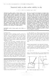
2.1 Structure <strong>of</strong> PSN. Assume that <strong>the</strong> number <strong>of</strong> neurons for <strong>the</strong> input,<br />
summation, and product layers are P, N, and 1, respectively. The structure is<br />
showninFigure1.Wedenotebywn = (wn1,wn2,...,wnP) T (1 ≤ n ≤ N)<strong>the</strong><br />
weight vector connecting <strong>the</strong> input and <strong>the</strong> summation node n, and write<br />
w = (w T 1 ,wT 2 ,...,wT N ) ∈ RNP . ξ = (ξ1,...,ξP) T ∈ R P stands for <strong>the</strong> input<br />
vector. Here we have added a special input unit ξP =−1 corresponding<br />
to <strong>the</strong> biases wnP. The weights on <strong>the</strong> connections between <strong>the</strong> product<br />
node and <strong>the</strong> summation nodes are fixed to 1. Let g : R → R be a given<br />
activation function for <strong>the</strong> output layer. For any given input ξ and weight<br />
w, <strong>the</strong> output <strong>of</strong> <strong>the</strong> network is<br />
�<br />
N�<br />
�<br />
y = g (wi · ξ) . (2.1)<br />
i=1<br />
2.2 Randomized Online Gradient Algorithm for PSN. The online<br />
gradient algorithm is a simple and efficient learning method for feedforward<br />
neural networks. Usually PSN and <strong>the</strong> networks with pi-sigma<br />
building blocks are also trained by it but with a randomized modification<br />
(or an asynchronous modification, which is not considered in this<br />
letter).
P1: SBQ<br />
07-06-285 NECO.cls July 26, 2007 9:38<br />
Online Gradient Algorithm for Pi-Sigma Network 3<br />
Figure 1: A pi-sigma network.<br />
Let {ξ j , O j } J j=1 ⊂ RP × R be <strong>the</strong> training examples. The usual mean<br />
square error function for <strong>the</strong> network is<br />
E(w) = 1<br />
2<br />
J�<br />
(O j − y j ) 2 = 1<br />
J�<br />
�<br />
O<br />
2<br />
j �<br />
N�<br />
− g (wi · ξ j ��2<br />
) . (2.2)<br />
j=1<br />
j=1<br />
The gradient <strong>of</strong> <strong>the</strong> error function with respect to wn (n = 1, 2,...,N)is<br />
DnE(w) =−<br />
J�<br />
�<br />
O j �<br />
N�<br />
− g (wi · ξ j ��<br />
) g ′<br />
j=1<br />
i=1<br />
�<br />
N�<br />
× (wi · ξ j �<br />
)<br />
⎛<br />
N� ⎜<br />
⎝ (wi · ξ j ⎞<br />
⎟<br />
) ⎠ ξ j . (2.3)<br />
i=1<br />
i=1<br />
i�=n<br />
The updating rule <strong>of</strong> <strong>the</strong> online gradient algorithm with a randomized<br />
modification for <strong>the</strong> weight vector <strong>of</strong> PSN is as follows (Shin & Ghosh, 1991).<br />
Start from an arbitrary initial guess w 0 .At<strong>the</strong>mth step (m = 0, 1,...)<strong>of</strong><strong>the</strong><br />
training iteration <strong>of</strong> <strong>the</strong> weights, we randomly choose an input example ξ j<br />
and a summing unit n and update <strong>the</strong> corresponding connecting weights<br />
while <strong>the</strong> weights <strong>of</strong> <strong>the</strong> o<strong>the</strong>r summing units remain unchanged, so <strong>the</strong><br />
online gradient algorithm iteratively updates <strong>the</strong> weights in <strong>the</strong> fashion<br />
that<br />
w m+1<br />
n = wm n + � jw m n (2.4a)<br />
w m+1<br />
q = wm q , q �= n (2.4b)<br />
i=1
P1: SBQ<br />
07-06-285 NECO.cls July 26, 2007 9:38<br />
4 Y. Xiong, W. Wu, X. Kang, and C. Zhang<br />
where<br />
� jw m �<br />
n = η O j �<br />
N�<br />
� m<br />
− g wi · ξ j���<br />
g ′<br />
i=1<br />
�<br />
N�<br />
� m<br />
× wi · ξ<br />
i=1<br />
j�� ⎛<br />
⎜<br />
⎝<br />
N� � m<br />
wi · ξ j�<br />
⎞<br />
⎟<br />
⎠ ξ j<br />
i=1<br />
i�=n<br />
(2.5)<br />
and η>0 is <strong>the</strong> learning rate.<br />
In this letter, we use C for a general positive constant, which may be<br />
different in different places but is independent <strong>of</strong> p, n, j, m, andη.<br />
2.3 Influence <strong>of</strong> Small Weights on <strong>the</strong> Training. Condition A on <strong>the</strong><br />
activation function <strong>will</strong> be needed in our analysis: |g(t)| and |g ′ (t)| are uniformly<br />
bounded for t ∈ R. It is satisfied by, for example, sigmoid functions,<br />
which are <strong>the</strong> most popular activation functions.<br />
Now let us illustrate <strong>the</strong> influence <strong>of</strong> <strong>the</strong> small weights on <strong>the</strong> training<br />
process. The following proposition estimates <strong>the</strong> magnitudes <strong>of</strong> <strong>the</strong><br />
increment <strong>of</strong> <strong>the</strong> weight vector � jw m n and <strong>the</strong> error function �E(wm ), respectively.<br />
Proposition 1. Let condition A be satisfied and <strong>the</strong> sequence {wm } ∞ m=1 be generated<br />
from <strong>the</strong> learning algorithm, 2.4. Then <strong>the</strong>re exists a positive constant C<br />
independent <strong>of</strong> η, n, p, j, andm, suchthat and<br />
�<br />
�� jw m �<br />
� N−1<br />
n ≤ Cηδm (2.6)<br />
|�E(w m 2(N−1 )<br />
)|≤Cηδm , (2.7)<br />
where δm = max<br />
1≤n≤N �wm n �, and δN−1 m<br />
2(N − 1)th powers <strong>of</strong> δm, respectively.<br />
2(N−1 )<br />
and δm denote <strong>the</strong> (N − 1 )th and<br />
Pro<strong>of</strong>. Estimate 2.6 can be obtained directly from <strong>the</strong> definition <strong>of</strong> δm,<br />
equation 2.5, and <strong>the</strong> Cauchy-Schwartz inequality.
P1: SBQ<br />
07-06-285 NECO.cls July 26, 2007 9:38<br />
Online Gradient Algorithm for Pi-Sigma Network 5<br />
To verify equation 2.7, we first expand �N i=1 (wm+1<br />
i<br />
<strong>the</strong> Taylor <strong>the</strong>orem:<br />
g<br />
� N�<br />
i=1<br />
� w m+1<br />
i<br />
i=1<br />
· ξ j )at � N<br />
i=1 wm n · ξ j by<br />
· ξ j��<br />
⎛<br />
⎜<br />
= g ⎝ �� w m n + � jw m� j<br />
n · ξ � N � � m<br />
wi · ξ j�<br />
⎞<br />
⎟<br />
⎠<br />
�<br />
N�<br />
� m<br />
= g wi · ξ j��<br />
+ g ′� t m ⎛<br />
�<br />
N�<br />
⎜ � m<br />
n, j ⎝ wi · ξ j�<br />
⎞<br />
⎟<br />
⎠ � � jw m n · ξ j� , (2.8)<br />
i=1<br />
i�=n<br />
where tm n, j is a real number between �N i=1 (wm+1<br />
i<br />
i=1<br />
i�=n<br />
· ξ j )and � N<br />
i=1 (wm i · ξ j ). Ac-<br />
cording to equation 2.6 and <strong>the</strong> Cauchy-Schwartz inequality, we have<br />
�<br />
�<br />
�<br />
�<br />
� g<br />
�<br />
N�<br />
� m+1<br />
wi · ξ j��<br />
�<br />
N�<br />
� m<br />
− g wi · ξ j��� �<br />
���<br />
≤ Cηδ 2(N−1)<br />
m max{g<br />
′ (x), �ξ j � N }<br />
i=1<br />
i=1<br />
This inequality, toge<strong>the</strong>r with equation 2.2, implies<br />
i=1<br />
i=1<br />
x∈R<br />
1≤ j≤J<br />
≤ Cηδ 2(N−1)<br />
m . (2.9)<br />
|�E(w m )|=|E(w m+1 ) − E(w m � �<br />
�<br />
�<br />
J�<br />
� �<br />
) �<br />
1 �<br />
�≤<br />
�<br />
� 2 � O<br />
j=1�<br />
j �<br />
N�<br />
� m+1<br />
− g wi · ξ<br />
i=1<br />
j���2<br />
�<br />
− O j �<br />
N�<br />
� m<br />
− g wi · ξ<br />
i=1<br />
j���2 � �<br />
����<br />
= 1<br />
�<br />
J�<br />
�<br />
�<br />
�<br />
2 �<br />
j=1�<br />
g<br />
�<br />
N�<br />
� m+1<br />
wi · ξ<br />
i=1<br />
j��<br />
�<br />
N�<br />
� m<br />
−g wi · ξ j�� �� �� ��� �<br />
�<br />
� O j �<br />
N�<br />
� m+1<br />
− g wi · ξ j��<br />
+ O j �<br />
N�<br />
� m<br />
− g wi · ξ j��� �<br />
���<br />
≤ CJηδ 2(N−1)<br />
m<br />
≤ Cηδ 2(N−1)<br />
m .<br />
It is well known that <strong>the</strong> initial guess w 0 ’s, and hence δ0, are required to be<br />
small in magnitude in order to avoid premature saturation <strong>of</strong> <strong>the</strong> weights.<br />
Then, we notice from equations 2.6 and 2.7 that � jw m n and �E(wm+1 )are<br />
even smaller when δm is small, resulting in a very slow convergence early in<br />
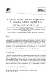
training. The situation <strong>will</strong> get worse for big N, as illustrated in Figure 2a.<br />
By proposition 1, a possible remedy might be to use a larger learning rate<br />
η to accelerate <strong>the</strong> convergence. This strategy is actually used in Shin and<br />
Ghosh (1992, 1995). But a constant large learning rate may lead to oscillation<br />
<strong>of</strong> <strong>the</strong> error function when <strong>the</strong> weights are not small, as illustrated in<br />
Figure 2(b).Thus, an adaptive variable learning rate seems desirable but is<br />
i=1
P1: SBQ<br />
07-06-285 NECO.cls July 26, 2007 9:38<br />
6 Y. Xiong, W. Wu, X. Kang, and C. Zhang<br />
Figure 2: The behaviors <strong>of</strong> PSN without penalty for a three-dimensional parity<br />
problem (cf. section 4.2). The number <strong>of</strong> neurons for <strong>the</strong> input and product<br />
layers are P = 4 and 1, respectively. The initial weights are selected randomly<br />
within <strong>the</strong> interval [−0.15, 0.15]. (a) The results <strong>of</strong> PSN with different numbers<br />
<strong>of</strong> summing units. The learning rate is 0.8 for (1) and 0.3 for (2) and (3). (1) N = 2;<br />
(2) N = 3; (3) N = 4. (b) The results <strong>of</strong> PSN with different learning rates. The<br />
number <strong>of</strong> summing units is N = 3: (1) η = 0.5; (2) η = 1.0; (3) η = 1.5.<br />
not easy to define directly. The above argument motivates us to introduce<br />
in <strong>the</strong> next section a penalty for small weights into <strong>the</strong> error function, so as<br />
to resolve <strong>the</strong> problem in an adaptive manner.<br />
3 Online Gradient Algorithm with a Penalty<br />
Recall that <strong>the</strong> original task <strong>of</strong> <strong>the</strong> network training is to <strong>find</strong> w∗ such that<br />
E(w∗ ) = min E(w). Now we add a constraint on<br />
w N�<br />
(w<br />
i=1<br />
m i · ξ j )toobtaina<br />
constrained optimization problem,<br />
min E(w)<br />
w<br />
�<br />
� N� �<br />
s.t. � (wi · ξ<br />
�<br />
j �<br />
�<br />
�<br />
) �<br />
�<br />
i=1<br />
>γ, j = 1, 2,...,J , (3.1)<br />
where γ>0 is an appropriate constant. This constrained optimization<br />
problem can be converted into a nonconstrained problem by using a Lagrangian<br />
multiplier λ:<br />
min<br />
w<br />
�E(w) ≡ min<br />
w<br />
⎧<br />
⎨<br />
λ<br />
E(w) +<br />
⎩ 2<br />
⎫<br />
J� ⎬<br />
p j(w) ,<br />
⎭<br />
(3.2)<br />
j=1
P1: SBQ<br />
07-06-285 NECO.cls July 26, 2007 9:38<br />
Online Gradient Algorithm for Pi-Sigma Network 7<br />
where λ>0 is <strong>the</strong> penalty coefficient, and p j(w) (j = 1, 2,...,J )is<strong>the</strong><br />
penalty function defined as<br />
⎧<br />
⎪⎨<br />
� �<br />
� N�<br />
p j(w) =<br />
γ − �<br />
� (wi · ξ<br />
⎪⎩<br />
i=1<br />
j ��2<br />
�<br />
) �<br />
� , −γ < N�<br />
(wi · ξ<br />
i=1<br />
j )
P1: SBQ<br />
07-06-285 NECO.cls July 26, 2007 9:38<br />
8 Y. Xiong, W. Wu, X. Kang, and C. Zhang<br />
be too big. On <strong>the</strong> o<strong>the</strong>r hand, λ needs to be large as usually required in<br />
optimization problems. A practical choice <strong>of</strong> γ and λ canbemadeinterms<br />
<strong>of</strong> experience or simulation experiment. Our experiments below indicate<br />
that <strong>the</strong> values <strong>of</strong> γ and λ can be chosen in a comparatively wide range.<br />
4 Simulation Results<br />
In this section, we test <strong>the</strong> performance <strong>of</strong> our penalty approach by two<br />
simulation examples. The training iteration process stops when one <strong>of</strong> <strong>the</strong><br />
following criteria is met:<br />
Criterion 1: The iteration step is less than 5000, and �△ jw m n � < 0.00001<br />
for three successive iterations.<br />
Criterion 2: �△ jw m n � < 0.00001 is not valid for three successive iterations,<br />
but <strong>the</strong> iteration step has reached 5000.<br />
4.1 Example 1: Function Approximation Problems. First, we trained<br />
<strong>the</strong> PSN to approximate <strong>the</strong> function f (x) = cos(π x/2), x ∈ [−1, 1]. The<br />
aim <strong>of</strong> this test is to compare <strong>the</strong> behaviors <strong>of</strong> <strong>the</strong> online gradient algorithms<br />
with or without penalty. The number <strong>of</strong> neurons for <strong>the</strong> input, summation,<br />
and product layers are P = 2, N = 3 and 1, respectively. The output activation<br />
function is g(x) = 1<br />
1+e−x . The parameters in this example take <strong>the</strong><br />
values η = 0.15, γ= 0.3, and λ = 40, and <strong>the</strong> initial weights are selected<br />
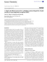
randomly within <strong>the</strong> interval [−0.15, 0.15]. Figure 3a shows <strong>the</strong> change <strong>of</strong><br />
<strong>the</strong> error function E(w) in <strong>the</strong> case without penalty, where <strong>the</strong> curve decreases<br />
slowly and keeps flat until <strong>the</strong> iteration step 4012. The value <strong>of</strong> <strong>the</strong><br />
product unit is accordingly small, as shown in Figure 3b. The result <strong>of</strong> <strong>the</strong><br />
online gradient algorithm with a penalty is shown in Figures 3c and 3d. The<br />
new error function ˜E(w) defined in equation 3.2 decreases fairly fast and<br />
meets Criterion 1 at iteration step 468.<br />
Next, we use <strong>the</strong> 2D Gabor function to show <strong>the</strong> function approximation<br />
capability <strong>of</strong> PSN with penalty. The 2D Gabor function has <strong>the</strong> following<br />
form (Shin & Ghosh, 1992):<br />
h(x, y) =<br />
�<br />
1<br />
x<br />
−<br />
· e<br />
2π(0.5) 2 2 +y2 2(0.5) 2<br />
�<br />
· cos(2π(x + y)).<br />
Thirty-six input points are selected from an evenly spaced 6 × 6gridon<br />
−0.5 ≤ x ≤ 0.5 and−0.5 ≤ y ≤ 0.5. Eighteen input points are randomly<br />
selected from <strong>the</strong> 36 points as <strong>the</strong> training set. The remaining 18 points are<br />
used for testing <strong>the</strong> generalization. The number <strong>of</strong> neurons for <strong>the</strong> input,<br />
summation, and product layers are P = 3, N = 6 and 1, respectively. The<br />
parameters in this example take <strong>the</strong> values η = 0.2, γ= 0.06, and λ = 15,<br />
and <strong>the</strong> initial weights are selected randomly within <strong>the</strong> interval [−2, 2].
P1: SBQ<br />
07-06-285 NECO.cls July 26, 2007 9:38<br />
Online Gradient Algorithm for Pi-Sigma Network 9<br />
Figure 3: Performances <strong>of</strong> online gradient algorithm (a, b) without penalty and<br />
(c, d) with penalty.<br />
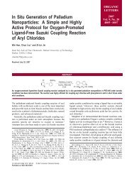
Figure 4: The approximation results for Gabor function: (a) Gabor function;<br />
(b) actual network outputs for PSN approximation with penalty; (c) actual<br />
network outputs for PSN approximation without penalty.<br />
The output activation function is g(x) = tanh (x). The errors <strong>of</strong> PSN with<br />
penalty for training and testing inputs achieve 0.098 and 0.89 after 2351<br />
epochs, while those <strong>of</strong> PSN without penalty are 0.1 and 0.88 after 4673<br />
epochs. Figure 4 shows <strong>the</strong> Gabor function and <strong>the</strong> actual network outputs.
P1: SBQ<br />
07-06-285 NECO.cls July 26, 2007 9:38<br />
10 Y. Xiong, W. Wu, X. Kang, and C. Zhang<br />
Figure 5: Performances <strong>of</strong> <strong>the</strong> online gradient algorithm (1) with penalty and<br />
(2) without penalty.<br />
Again we see from <strong>the</strong> experiment that our penalty algorithm can expedite<br />
<strong>the</strong> training <strong>of</strong> PSN.<br />
4.2 Example 2: K-Dimensional Parity Problems. The K-dimensional<br />
parity problem is a difficult classification problem. There are 2K -input patterns<br />
in <strong>the</strong> K -dimensional vector space. The values <strong>of</strong> <strong>the</strong> components <strong>of</strong><br />
<strong>the</strong> input patterns are ei<strong>the</strong>r +1 or−1. The output is 1 when <strong>the</strong> input pattern<br />
contains an odd number <strong>of</strong> +1 ′ s and is −1 o<strong>the</strong>rwise. The famous XOR<br />
problem is just <strong>the</strong> two-dimensional parity problem. In <strong>the</strong>se experiments,<br />
<strong>the</strong> output activation function is g(x) = 1<br />
1+e−x .<br />
First, we investigate <strong>the</strong> behaviors <strong>of</strong> PSN with or without penalty for<br />
<strong>the</strong> three-dimensional parity problem. The number <strong>of</strong> neurons for <strong>the</strong> input,<br />
summation, and product layers are P = 4, N = 3 and 1, respectively. The<br />
initial weights are selected randomly within <strong>the</strong> interval [−0.15, 0.15]. The<br />
parameters in this example are η = 0.2, γ= 0.05, and λ = 10. The result is<br />
shown in Figure 5.<br />
Next, we investigate <strong>the</strong> behaviors <strong>of</strong> <strong>the</strong> two approaches, using ei<strong>the</strong>r<br />
a large learning rate or a penalty respectively, for <strong>the</strong> four-dimension<br />
parity problem. The number <strong>of</strong> neurons for <strong>the</strong> input, summation and<br />
product layers are P = 5, N = 4 and 1, respectively. The parameters are<br />
w ∈ [−0.2, 0.2], γ= 0.05, and λ = 10. Ten tests are carried out with different<br />
parameters. It is clear from Figure 6 that <strong>the</strong> penalty approach has<br />
better convergence and stability as η ∈ [0.3, 0.5] than <strong>the</strong> large learning rate<br />
approach as η ∈ [1.0, 1.4].<br />
Finally, we choose different values <strong>of</strong> λ and γ to test <strong>the</strong>ir influence on <strong>the</strong><br />
performance <strong>of</strong> <strong>the</strong> online gradient algorithm with a penalty for <strong>the</strong> fourdimension<br />
parity problem. Ten tests are carried out with different values <strong>of</strong>
P1: SBQ<br />
07-06-285 NECO.cls July 26, 2007 9:38<br />
Online Gradient Algorithm for Pi-Sigma Network 11<br />
Figure 6: Performances <strong>of</strong> <strong>the</strong> online gradient algorithm (a, b) without penalty<br />
and (c, d) with penalty.<br />
Table 1: Number <strong>of</strong> Successful Tests in 10 Tests.<br />
λ = 4 λ = 8 λ = 12 λ = 16 λ = 20 λ = 24 λ = 28 λ = 32 λ = 36<br />
γ = 0.01 6 6 1 6 4 8 4 6 2<br />
γ = 0.02 4 6 4 6 5 6 5 4 4<br />
γ = 0.03 1 9 5 6 6 5 5 3 4<br />
γ = 0.04 6 6 5 5 7 4 3 6 5<br />
γ = 0.05 4 7 6 5 6 8 3 3 2<br />
γ = 0.06 5 3 5 5 4 2 3 2 2<br />
γ = 0.07 6 5 5 5 4 5 3 5 3<br />
γ = 0.08 9 5 5 3 5 1 0 1 1<br />
γ = 0.09 7 4 1 3 1 3 1 2 1<br />
λ and γ . The number <strong>of</strong> <strong>the</strong> successful tests—namely, <strong>the</strong> tests that stop by<br />
criterion 1—in <strong>the</strong> 10 tests are given in Table 1. The average stopping steps<br />
<strong>of</strong> <strong>the</strong> 10 tests are showed in Table 2. We observe that λ in [8, 24] and γ in<br />
[0.01, 0.05] give better convergence and stability.
P1: SBQ<br />
07-06-285 NECO.cls July 26, 2007 9:38<br />
12 Y. Xiong, W. Wu, X. Kang, and C. Zhang<br />
Table 2: Average Iteration Steps <strong>of</strong> 10 Tests.<br />
λ = 4 λ = 8 λ = 12 λ = 16 λ = 20 λ = 24 λ = 28 λ = 32 λ = 36<br />
γ = 0.01 3124 3447 4808 3893 3871 3051 4459 3539 4428<br />
γ = 0.02 3976 3439 3961 3350 2562 3864 3405 3598 3734<br />
γ = 0.03 4859 2834 3506 3038 3131 3175 4066 4242 3615<br />
γ = 0.04 3700 3663 3660 3869 3725 2732 4111 3036 3173<br />
γ = 0.05 3807 3123 3133 3253 2516 3168 3959 3909 4449<br />
γ = 0.06 3625 4030 3367 3475 3456 4245 3903 4173 4248<br />
γ = 0.07 3596 3393 3379 3252 3677 3743 3986 3116 3812<br />
γ = 0.08 2886 3235 3788 4100 3429 4566 5000 4563 4575<br />
γ = 0.09 3253 3559 4558 3952 4697 4554 4693 4491 4534<br />
Acknowledgments<br />
This work was partly supported by <strong>the</strong> National Natural Science Foundation<br />
<strong>of</strong> China (10471017).<br />
References<br />
Durbin, R., & Rumelhart, D. (1989). Product units: A computationally powerful and<br />
biologically plausible extension to backpropagation networks. Neural Computation,<br />
1, 133–142.<br />
Giles, C. L., & Maxwell, T. (1987). Learning invariance and generalization in higherorder<br />
neural networks. Applied Optics, 26(23), 4972–4978.<br />
Hussaina, A. J., & Liatsisb, P. (2002). Recurrent pi-sigma networks for DPCM image<br />
coding. Neurocomputing, 55, 363–382.<br />
Jiang, L. J., Xu, F., & Piao, S. R. (2005). Application <strong>of</strong> pi-sigma neural network to<br />
real-time classification <strong>of</strong> seafloor sediments. Applied Acoustics, 24, 346–350.<br />
Li, C. K. (2002). Memory-based sigma-pi-sigma neural network. International Conference<br />
on Systems, Man and Cybernetics, 4, 1–6.<br />
Li, C. K. (2003). A sigma-pi-sigma neural network (SPSNN). Neural Processing Letters,<br />
17, 1–19.<br />
Shin, Y., & Ghosh, J. (1991). The pi-sigma network: An efficient higher-order neural<br />
network for pattern classification and function approximation. International Joint<br />
Conference on Neural Networks, 1, 13–18.<br />
Shin, Y., & Ghosh, J. (1992). Approximation <strong>of</strong> multivariate functions using ridge<br />
polynomial networks. In Proceedings <strong>of</strong> International Joint Conference on Neural<br />
Networks (Vol. 2, pp. 380–385). Piscataway, NJ: IEEE Press.<br />
Shin, Y., & Ghosh, J. (1995). Ridge polynomial networks. IEEE Transactions on Neural<br />
Networks, 6(3), 610–622.<br />
Sinha, M., Kumar, K., & Kalra, P. K. (2000). Some new neural network architectures<br />
with improved learning schemes. S<strong>of</strong>t Computing, 4(4), 214–223.<br />
Voutriaridis, C., Boutalis, Y. S., & Mertzios, B. G. (2003). Ridge polynomial networks<br />
in pattern recognition. In 4th EURASIP Conference Focused on Video I Image
P1: SBQ<br />
07-06-285 NECO.cls July 26, 2007 9:38<br />
Online Gradient Algorithm for Pi-Sigma Network 13<br />
Processing and Multimedia Communications (Vol. 2, pp. 519–524). Piscataway, NJ:<br />
IEEE Press.<br />
Xin, L. (2002). Interpolation by ridge polynomials and its application in neural<br />
networks. Journal <strong>of</strong> Computational and Applied Ma<strong>the</strong>matics, 144, 197–209.<br />
Received July 21, 2006; accepted January 24, 2007.